An Estimator for Pairwise Relatedness Using Molecular Markers
Jinliang Wang
1Institute of Zoology, Zoological Society of London, London NW1 4RY, United Kingdom
Manuscript received June 22, 2001 Accepted for publication December 12, 2001
ABSTRACT
I propose a new estimator for jointly estimating two-gene and four-gene coefficients of relatedness between individuals from an outbreeding population with data on codominant genetic markers and compare it, by Monte Carlo simulations, to previous ones in precision and accuracy for different distribu-tions of population allele frequencies, numbers of alleles per locus, actual reladistribu-tionships, sample sizes, and proportions of relatives included in samples. In contrast to several previous estimators, the new estimator is well behaved and applies to any number of alleles per locus and any allele frequency distribution. The estimates for two- and four-gene coefficients of relatedness from the new estimator are unbiased irrespective of the sample size and have sampling variances decreasing consistently with an increasing number of alleles per locus to the minimum asymptotic values determined by the variation in identity-by-descent among lociper se, regardless of the actual relationship. The new estimator is also robust for small sample sizes and for unknown relatives being included in samples for estimating allele frequencies. Compared to previous estimators, the new one is generally advantageous, especially for highly polymorphic loci and/ or small sample sizes.
G
ENETIC relationships among individuals within ment estimators for two-gene and four-gene relatedness have been proposed (e.g.,Lynch 1988; Queller and and between populations play a pivotal role inquantitative genetics, conservation genetics, and many Goodnight1989;Liet al.1993;Ritland1996b;Lynch andRitland1999), and their performances have been areas of evolution and ecology (Ritland1996a,b, 2000;
LynchandRitland1999). Such relationships can be compared in recent studies (LynchandRitland1999; Van de Casteeleet al.2001). In this article I develop easily estimated from pedigree information. For natural
populations, however, detailed knowledge of pedigree a new estimator for simultaneously estimating two-gene and four-gene coefficients of relatedness between a pair is usually unavailable. Genetic markers can be used,
instead, to infer the relationships among individuals of individuals and evaluate its performance against pre-vious estimators for different actual relationships and without pedigree information.
Marker-based methods for inferring genetic relation- allele frequency distributions in the population. LynchandRitland(1999) assessed the previous mo-ships among individuals can be categorized into two
groups. The first group uses a likelihood approach to ment estimators assuming that the allele frequencies of the population were known. In practice, however, the determine the likelihood of a pair of individuals falling
into a particular type of relationship (such as full-sibs, allele frequencies of the population have to be estimated from samples and are therefore subject to sampling parent-offspring, etc.) given the marker data (e.g.,
Thomp-son1975;Marshallet al.1998;Mousseauet al.1998; errors. For highly polymorphic markers (e.g., microsatel-lites) and realistic sample sizes, the sampling errors for Goodnight and Queller 1999; Thomas and Hill
2000). The second group uses moment estimators to allele frequency cannot be ignored in comparing the performances of the estimators. Little is known about estimate the relatedness between a pair of individuals,
which is a continuous quantity defined in terms of prob- the sensitivities of these moment estimators for relat-edness to the sampling errors in allele frequency. In abilities of identity-by-descent (e.g.,Lynch1988;Queller
andGoodnight1989; Liet al. 1993; Ritland1996b; this article, I compare the accuracy and precision of LynchandRitland1999). different estimators of relatedness when allele frequen-Relatedness estimators are especially useful for popu- cies are estimated from samples and when unknown lations with complex (unknown) pedigrees or with little relatives are included in the samples. I show that the prior information on population structure. Several mo- new moment estimator can easily take the effect of small sample size into account. Compared to the other estima-tors, the new one is well behaved irrespective of the number of alleles per locus, the allele frequency distri-bution, sample size, and the inclusion of relatives in
1Address for correspondence :Institute of Zoology, Regent’s Park,
Lon-don NW1 4RY, United Kingdom. E-mail: [email protected] samples for estimating allele frequencies.
THE NEW ESTIMATOR OF TWO-GENE AND
P1⫽
兺
ni⫽1
P(ii,ii)⫹
兺
ni⫽1
兺
nj⬆i⫽1
P(ij,ij)⫽b⫹cφ⫹(1⫺b)⌬, FOUR-GENE COEFFICIENTS OF RELATEDNESS
The coefficients of relatedness: Following previous (2)
studies, I consider an outbred diploid population
through-where b ⫽ 2a2
2 ⫺ a4, c ⫽ a2 ⫺ 2a22 ⫹ a4 in which the
out. A pair of individuals (say,xandy) in such a
popula-sum of powers of gene frequencyam⫽
兺
ni⫽1pmi form⫽ tion can be genetically correlated in two ways: a single
2, 3, and 4. The probabilities for categories 2–4 are gene at a locus inxis identical by descent with one in
y, or both genes inxare identical by descent with those
P2⫽
兺
ni⫽1
兺
nj⬆i⫽1
P(ii,ij)⫽ d(1⫺ ⌬)⫹ eφ, (3) iny.If the probabilities of occurrences of the first and
second events are denoted as φ and ⌬, respectively,
whered ⫽4(a3 ⫺a4) ande⫽2(a2⫺3a3⫹2a4);
the relatedness,r, between individuals xandy can be expressed as
P3 ⫽
兺
ni⫽1
兺
nj⬆i⫽1
兺
nk⬆i⬆j⫽1
P(ij,ik)⫽f(1⫺ ⌬)⫹gφ, (4)
r⫽ φ/2 ⫹ ⌬ (1)
wheref⫽4(a2⫺a22⫺2a3⫹2a4) andg⫽(1⫺7a2⫹
(LynchandRitland1999). In an outbreeding
popula-4a2
2⫹10a3⫺8a4); and
tion,φ,⌬, andrare 1, 0, and 0.5, respectively, for parents and offspring; 0.5, 0.25, and 0.5, respectively, for full- P
4 ⫽
兺
n
i⫽1
兺
nj⬆i⫽1
P(ii,jj)⫹
兺
ni⫽1
兺
nj⬆i⫽1
兺
nk⬆i⬆j⫽1 P(ii,jk) sibs; and 0.25, 0, and 0.125, respectively, for half-sibs.
Although φ, ⌬, and r can be estimated for any pair
⫹
兺
ni⫽1
兺
nj⬆i⫽1
兺
nk⬆i⬆j⫽1
兺
nl⬆k⬆i⬆j⫽1
P(ij,kl) of individuals using genotypic data, I concentrate on
the estimation of ⌬ and r only because these two are
⫽(1⫺ 4a2 ⫹2a22⫹4a3⫺3a4)(1⫺φ⫺ ⌬), (5)
used to partition the genetic variance of a quantitative trait (2
G) into the additive (2A)and dominance (D2) respectively. Obviously, we haveP
1⫹P2⫹P3⫹P4⬅1,
components,2
G⫽ r2A⫹ ⌬D2(FalconerandMackay because a pair of genotypes must fall into one of the
1996;LynchandWalsh1998). Furthermore, the esti- four categories. The observed values (denoted asPˆ i) of mates ofφhave a much higher sampling variance than Pi (i ⫽1, 2, 3, or 4) for a pair of genotypes constitute those of ⌬ andr (Lynchand Ritland 1999). Unless the data; one of the four values is one and the rest are data on a very large number of informative loci are zero. For example, if we observe
AiAi-AiAi orAiAj-AiAj, available,φcannot be estimated with reasonable confi- then
Pˆ1 ⫽1 andPˆ2⫽Pˆ3⫽Pˆ4⫽0.
dence. For biallelic loci (
n⫽ 2), category 3 is not possible,
The new estimator: To derive the new estimator, I and only three equations remain to be solved for param-first determine the joint probabilities of two genotypes etersφand⌬. Solving any two of the three dependent given the parametersφand⌬(to be estimated) and the equations yields
allele frequencies of the population (assumed to be
known for this section). For a marker locus withn co- φˆ ⫽(4 ⫺4Pˆ1⫺ 3Pˆ2)(1⫺a2)⫺4(1⫺ Pˆ1⫺ Pˆ2)
(1⫺a2)2
, (6) dominant alleles indexed by i, j, k, l ⫽ 1, 2, . . . , n,
there would be n(n ⫹ 1)/2 possible genotypes and
n(n ⫹ 1)[n(n ⫹ 1) ⫹ 2]/8 possible combinations of ⌬ˆ ⫽1⫺(4 ⫺4Pˆ1⫺ 3Pˆ2)(1⫺a2)⫺2(1⫺ Pˆ1⫺Pˆ2) (1⫺a2)2
. genotypes for a pair of individuals. The probabilities of
these combinations of genotypes can be derived in terms (7)
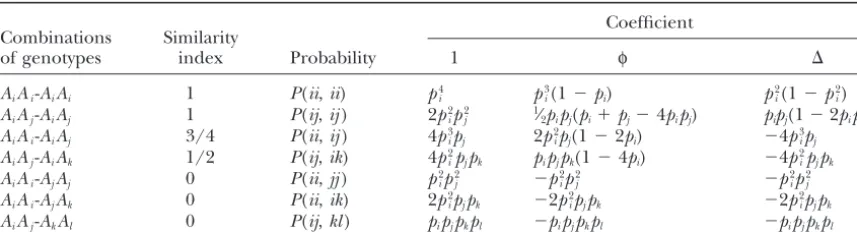
ofφ,⌬, and allele frequencies, as are listed in Table 1
Inserting (6) and (7) into (1) yields where the population frequency of alleleAiis denoted
aspi.According to their similarity index S, defined as
rˆ⫽4Pˆ1⫹ 3Pˆ2⫺2(1⫹ a2) 2(1⫺a2)
. (8)
the arithmetic average fraction of genes at a locus in a reference individual (here eitherxory) for which there
Equation 7 for⌬is essentially the same as that ofLynch is another gene in the other individual (either yor x)
andRitland(1999, their Equation 4b) for biallelic loci. that is identical in state (Lynch 1988; Li et al. 1993),
Equations 6 and 8 for φand r are, however, different these genotype combinations can be grouped into four
from those ofLynchandRitland(1999). Equation 8 categories. Category 1 contains combinations AiAi-AiAi
for r is essentially the same as Equation 9 of Li et al. andAiAj-AiAjwith S⫽1; category 2 contains
combina-(1993) for the case of biallelic loci, which was developed tionsAiAi-AiAjwithS⫽3⁄
4; category 3 contains
combina-with a modification of the similarity index for category tionsAiAj-AiAkwith S ⫽ 1⁄
2; category 4 contains all the
3 ofLynch(1988). The new estimator is advantageous rest of the combinations withS⫽ 0 (i⬆ j⬆ k⫽1, 2,
in that it can estimateφand⌬as well. . . . ,n). Summing up the probabilities of all the genotype
With a multiallelic locus, there are more indepen-combinations within a category gives the probability of
dent equations than the parameters to be estimated. A occurrence of that category. The probability of
TABLE 1
Probabilities of a pair of genotypes at a diploid marker locus withncodominant alleles (i⬆j⬆k⬆l⫽1, 2, . . . ,n)
Coefficient Combinations Similarity
of genotypes index Probability 1 φ ⌬
AiAi-AiAi 1 P(ii,ii) p4i p3i(1⫺pi) p2i(1⫺p2i)
AiAj-AiAj 1 P(ij,ij) 2p2ip2j 1⁄2pipj(pi⫹pj⫺4pipj) pipj(1⫺2pipj) AiAi-AiAj 3/4 P(ii,ij) 4p3ipj 2p2ipj(1⫺2pi) ⫺4p3ipj AiAj-AiAk 1/2 P(ij,ik) 4p2ipjpk pipjpk(1⫺4pi) ⫺4p2ipjpk
AiAi-AjAj 0 P(ii,jj) p2ip2j ⫺p2ip2j ⫺p2ip2j
AiAi-AjAk 0 P(ii,ik) 2pi2pjpk ⫺2p2ipjpk ⫺2p2ipjpk
AiAj-AkAl 0 P(ij,kl) pipjpkpl ⫺pipjpkpl ⫺pipjpkpl
the estimates ofφand⌬(and thusr) with the minimum moments of allele frequency in Crow and Kimura (1970, p. 335, correcting for the typographical error in sampling variance. Unfortunately, however, the
opti-mum weights must be obtained from the variance-covar- the fourth moment). These are iance matrix, which depends on the unknown
parame-tersφand⌬. To obtain approximate weights, I follow a2 ⫽Naˆ2 ⫺1
N⫺1 , (12)
Ritland(1996b) and Lynch andRitland (1999) in assuming thatφ⫽ ⌬ ⫽0 in the absence of prior
informa-a3 ⫽ N2aˆ
3⫺3(N⫺1)a2⫺1
(N⫺1)(N ⫺2) , (13)
tion on the relationship. With this assumption I can obtain the weighted least-squares estimators ofφand⌬ from (2–5) using an equation-solving software,
a4 ⫽ N3aˆ
4⫺ 6(N⫺ 1)(N⫺2)a3⫺ 7(N⫺ 1)a2⫺ 1
N3⫺6N2 ⫹11N ⫺6 .
φ
ˆ ⫽
兵
df[(e⫹g)(1⫺b)⫹c(d ⫹f)](Pˆ1⫺ 1)(14)
⫹ d(1⫺ b)[g(1⫺b⫺ d)⫹f(c ⫹e)]Pˆ3
As is shown below, essentially unbiased estimates of
relat-⫹ f(1 ⫺b)[e(1 ⫺b⫺f)⫹d(c⫹g)]Pˆ2
其
/V,edness can be obtained with the new estimator using (9) (9–14), irrespective of the sample sizeN.
In practice, relatedness is estimated using several loci.
⌬ˆ ⫽
兵
cdf(e⫹g)(Pˆ1⫹1⫺2b) Although relatedness estimates from unlinked loci in linkage equilibrium are independent, they could bedra-⫹[(1⫺b)(fe2⫹dg2)⫺(ef⫺dg)2](Pˆ 1⫺b)
matically different in sampling variance and ideally should not be simply averaged to give the overall
esti-⫹c(dg⫺ef)(dPˆ3⫺f Pˆ2)⫺c2df
mate. The optimum weights among loci are difficult to
⫻(Pˆ3⫹Pˆ2⫺d⫺f)⫺c(1⫺b)(dgPˆ3⫹ef Pˆ2)
其
/V,obtain for any moment estimator, however, because they are functions of the parameters (φ and ⌬) being esti-(10)
mated. As a result, the difference in the amount of where
information among loci was either ignored by using equal weights (e.g.,QuellerandGoodnight1989;Liet V⫽ (1⫺b)2(e2f⫹dg2)⫺(1 ⫺b)(ef⫺ dg)2
al.1993) or taken partially into account by approximate
⫹2cdf(1⫺ b)(g⫹e)⫹c2df(d⫹f), (11)
weights derived assuming null relatedness, such as heter-ozygosity (Loiselleet al.1995), number of alleles at a and b–g are defined in (2–4). Inserting (9) and (10)
locus (Ritland 1996a,b), or the inverse of sampling into (1) yields the estimate forr.
variance for nonrelatives (LynchandRitland1999). When allele frequencies for the population are
un-None of the weighting methods is appropriate in all known but are estimated from a sample of N genes
circumstances (allele frequency distribution, actual rela-taken at random from the population, the sampling
tionship), as is intuitively obvious. Methods with equal error should be taken into account. Denoting the
sam-weighting (e.g.,Queller and Goodnight1989; Li et ple allele frequency for alleleAiaspˆi, the observed sums
of powers of allele frequencies areaˆm⫽
兺
ni⫽1pˆmi form⫽ al. 1993) tend to give higher sampling variances for nonrelatives and lower sampling variances for relatives, 2, 3, and 4. Obviously,aˆmis a biased estimate ofamfor
compared to the weighting methods based on the sam-the population. The expected sums of powers of allele
pling variance of nonrelatives (Ritland1996a,b;Lynch frequencies (denoted asamform⫽2, 3, and 4) can be
meth-ods in the new estimator and found the following cause it is quite complex algebraically and involves the solution for weights of two sets of n(n ⫹ 5)/2 linear method is more satisfactory in the vast majority of cases
considered in simulations. equations for a single locus withnalleles.
On the basis of probability of a genotype conditional The average similarity value for unrelated individuals
isu⫽2a2⫺a3(Liet al.1993), which is due completely on the reference genotype, allele frequencies pi, and
parametersr and⌬, LynchandRitland (1999) pro-to chance (identity-in-state) and determined solely by
allele frequencies at a locus. The amount of information posed a much simpler “regression” estimator (denoted as LR). For a single locusl, the estimates of relatedness for a locus in estimating relatedness decreases with an
increasing value ofu.Therefore I use a weight for locus between individualsxandyusingxas the reference are l asw(l) ⫽ 1/(Uul), whereU is the sum of 1/ul over
rˆxy(l)⫽
pa(Sbc⫹Sbd)⫹pb(Sac⫹Sad)⫺4papb
(1⫹Sab)(pa⫹pb)⫺4papb
, (17) loci. The averages ofPˆi(i⫽1, 2, and 3), am(m⫽ 2, 3,
and 4), anda2
2 weighted byw(l) over loci are used in
the new estimator. If allele frequencies are estimated ⌬ˆxy(l)⫽2papb⫺pa(Sbc⫹Sbd)⫺pb(Sac⫹Sad)⫹SacSbd⫹SadSbc
(1⫹Sab)(1⫺pa⫺pb)⫹2papb
, from samples, am anda2
2 are calculated using (12–14)
(18) for each locus and then weighted over loci for use in
the estimation. where indicator variables Sij (i, j ⫽ a, b, c, or d) are
defined in (16). For a number ofLloci, the composite estimates are obtained by weighting single-locus esti-COMPARISON AMONG ESTIMATORS
mates across loci, Several moment estimators for pairwise relatedness
have been proposed, which are summarized and com- rˆxy⫽ 1
Wr,x
兺
Ll⫽1
wr,x(l)rˆxy(l), (19) pared byLynchandRitland(1999). For convenience,
these estimators are briefly described below.
⌬ˆxy⫽ 1 W⌬,x
兺
L
l⫽1
w⌬,x(l)⌬ˆxy(l), (20) Based on the similarity index, or the sharing of genes
between individuals,Lynch(1988) developed an
esti-mator forr, which was later improved byLiet al.(1993). where the weights for locusl, This estimator (denoted as LL hereafter) is
wr,x(l)⫽
(1⫹Sab)(pa⫹pb)⫺ 4papb
2papb , (21)
rˆ⫽(Sxy⫺ u)/(1⫺u), (15)
where Sxyis the similarity index between individuals x
w⌬,x(l)⫽
(1⫹ Sab)(1⫺ pa⫺pb)⫹ 2papb
2papb (22)
andy(as defined in Table 1), andu⫽ 2a2⫺ a3is the
average similarity among unrelated individuals due to
chance. are derived by assuming that x and y are unrelated
Queller and Goodnight’s (1989) estimator (de- (LynchandRitland1999). In (19) and (20),Wr,xand noted as QG) for the average relatedness between W
⌬,x are the sums of weights over the L loci. Using groups of individuals can also be made to estimate the individual y as the reference, the estimates rˆyx and⌬ˆ
yx pairwiser, as shown byLynchandRitland(1999). Let can be obtained similarly. The arithmetic average of the individualsxandyhave genesa,bandc,d, respectively, reciprocal estimates rˆyx andrˆxy (⌬ˆ
xy and ⌬ˆyx) yields the at a locus and indicator variables Sij ⫽ 1 if gene i is estimate ofr(⌬) between individualsxandy.
identical in state to genej(i,j⫽a,b,c, ord) andSij⫽ Compared to the other estimators, an attractive prop-0 otherwise. The estimate ofrxyusing individualxas the erty of the new estimator (denoted as W) and the QG
reference is and LL estimators is that they do not give estimates of
r⬎1. Like the other estimators, however, they do yield rˆxy⫽ 0.5(Sac⫹Sad⫹ Sbc⫹ Sbd)⫺pa⫺ pb
1⫹Sab⫺ pa⫺pb , (16) negative estimates because of sampling error. The new estimator does not generate estimates of⌬ ⬎1 except for biallelic loci (in which case the maximum estimate where piis the frequency of allelei. Similarly,rˆyxusing
individualyas the reference can be obtained from (16), for⌬is 2.125), in contrast to the LR and R estimators. In the following, I compare the precision and accu-replacingSabbyScdandpaandpbbypcandpd, respectively.
The arithmetic average of the reciprocal estimates racy of these estimators for different actual relationships and allele frequency distributions. First I assume that rˆyxandrˆxyyields the estimate ofrbetween individualsx
andy. the allele frequencies of the population are known, and
then I assume that allele frequencies are estimated from For estimating r and ⌬ simultaneously, Ritland
(1996b) developed a “correlation” estimator (denoted samples taken binomially from the population without and with relatives-clusters included in them.
as R) on the basis of the joint distributions of both
be-pairwise relatedness estimators are essentially unbiased, that, for some allele frequencies, they are undefined because the denominator becomes zero. For biallelic regardless of the allele frequencies, number of loci, and
the actual relationship (LynchandRitland1999; data loci, the QG estimator is undefined when the reference individual is a heterozygote. When the allele frequencies not shown). I, therefore, concentrate on evaluating the
estimators in their precision, which is indicated by the are exactly equal for biallelic loci and the reference genotype is a heterozygote, the LR estimator yields un-sampling variance of the estimates given the actual
rela-tionship and allele frequencies. defined estimates. Some equations in the R estimator are invalid when the allele frequency is either 0.5 or For all of the estimators except for the LR estimator,
the average single-locus sampling variance, calculated 0.25. Allele frequencies near these values cause errati-cally very large estimates from the three estimators be-as the variance of multilocus estimates divided by the
number of loci, is independent of the number of loci. cause the denominator is close to zero. This is paradoxi-cal because an allele frequency of 0.5 gives the maximum Given the allele frequencies and the actual relationship,
I can obtain the probability of each pair of genotypes heterozygosity (for the allele in question) and thus should yield the best estimation. In the following, I at a single locus and thus the exact sampling variance
of relatedness estimates from each estimator. avoid biallelic loci in the QG estimator and ignore those component estimates in the R and LR estimators when-For the LR estimator, however, the average
single-locus sampling variance changes with the number of ever they “blow up.”
With known allele frequencies in proportions 1, 2, 3, loci used in the estimation, because the weights for
different loci depend in part on the reference genotypes . . . ,n(triangular distribution), the five estimators are compared in precision for different numbers of alleles at the corresponding loci (LynchandRitland1999).
I used Monte Carlo simulations to generate paired per locus (Figure 1). For the estimation ofr, estimators W, LL, and QG give essentially the same results for multilocus genotypes conditional on the allele
frequen-cies and the actual relationship. The sampling variance nonrelatives (almost indistinguishable in the graph) and very similar results for relatives when the number was calculated from the relatedness estimates for at least
100,000 pairs of individuals. For simplicity hereafter, the of alleles is large. If the number of alleles is small (n⬍ 5), however, the QG estimator yields higher sampling average locus sampling variance is called
single-locus sampling variance, bearing in mind that it is esti- variances. For nonrelatives, the LR and R estimators have basically the same precision, which is slightly mated from multiple loci and varies with the number
of loci for the LR estimator. higher than that of the other three estimators across
the range of the number of alleles. For relatives, how-A peculiar property of the LR estimator is that the
single-locus sampling variances of both r and ⌬ for ever, the LR and R estimators result in much larger sampling variances than the other estimators whennis related individuals may increase with an increasing
num-ber of loci. Extensive simulations show that the phenom- large. The sampling variance ofrfor either full-sibs or parent-offspring nearly levels off for the LR estimator enon happens more often with a closer actual
relation-ship and a larger number of alleles per locus (data not and is actually increasing for the R estimator, when n increases above the value of 12.
shown). Allele frequency distributions also affect the
direction (increasing or decreasing) of the changes in For the estimation of⌬, the W estimator gives slightly worse estimates for nonrelatives, slightly better estimates single-locus variance with an increasing number of loci,
as can be seen from Figure 1 inLynchand Ritland for parent-offspring, and much better estimates for full-sibs where the expected value of⌬is greater than zero. (1999). Furthermore, the single-locus variance may not
be able to reach an asymptotic value with an increasing With full-sibs, the sampling variance for the R estimator begins to increase withn when it is⬎6.
number of loci. If 1, 5, 10, 20, 40, and 80 loci [each
having 10 alleles with known frequencies in proportions As is intuitively obvious, an increase in the number of alleles per locus should reduce the sampling variance 1, 2, . . . , 10 (triangular distribution)] are used in
estimating the relatedness for full sibs, for example, the of relatedness estimates, because alleles identical in state are more reliable as indicators of identity-by-descent. single-locus sampling variances for⌬are 0.27, 0.36, 0.42,
0.49, 0.55, and 0.62, respectively. The total sampling The phenomenon that the sampling variance of relat-edness (ror⌬) for relatives from the R and LR estima-variance always decreases but at a decelerating rate with
an increasing number of loci. For nonrelatives, the sin- tors does not decrease consistently with an increasing number of alleles is perhaps caused by the assumptions gle-locus sampling variance always decreases to an
asymptotic value with an increasing number of loci. The made in deriving weights in these estimators. Without prior information, it is reasonable to assumer⫽0 and odd behavior of the LR estimator is perhaps due to the
weights among loci, which are obtained by assuming ⌬ ⫽ 0 for deriving weights among loci (Lynch and Ritland1999) and among component equations within r⫽ 0 and ⌬ ⫽ 0 (Lynchand Ritland1999). In the
comparison below, I followLynchandRitland(1999) a locus (Ritland 1996b; Lynch and Ritland 1999). With an increasing number of alleles, there would be in using 10 loci in the estimation for the LR estimator.
Figure1.—Single-locus sampling variances for estimates ofrand ⌬as a function of the number of alleles per locus. The sampling vari-ances ofrestimates are obtained from the new estimator (W),LynchandRitland’s (1999) estimator (LR),Ritland’s (1996b) estimator (R),Lynch(1988) andLiet al.’s (1993) esti-mator (LL), andQuellerandGoodnight’s (1989) estimator (QG); those of⌬ estimates are obtained from W, LR, and R estimators, assuming known allele frequencies in a trian-gular distribution. The results for the LR esti-mator are obtained by Monte Carlo simula-tions on 10 loci, those from the other estimators are exact solutions based on proba-bilities of genotype combinations given allele frequency distribution and actual relationship. Note that both axes are in log scale, and the sampling variances forrestimates of nonrela-tives are similar and indistinguishable between the LR and R estimators and among W, LL, and QG estimators.
used under the assumption. Although I made the same assumption in deriving weights for the two estimators. The optimum weights are a function of the relationship assumption in the new estimator, there are only a fixed
number of 3 equations used in the estimation, irrespec- being estimated. Although one can refine the weights iteratively from a starting prior relationship (say,r⫽0 tive of the number of alleles (except forn ⫽ 2 where
no weight is involved). In contrast, there aren(n⫹5)/ and ⌬ ⫽ 0) and use the values when an appropriate degree of convergence has been reached, the resultant 2 equations (weights) for a single locus with n alleles
in the R estimator and 5 (if the reference genotype is estimates are generally much worse even if one uses a large number of loci (Ritland 1996a,b; Lynch and a heterozygote) plus the number of weights equivalent
to the number of loci in the LR estimator. For a given Ritland1999; data not shown).
Simulations were also run to compare these estima-allele frequency distribution, the frequency of
heterozy-gotes and thus the number of weights in the LR estima- tors for other distributions of allele frequencies. With each of thenalleles being equal to 1/n, the same trend tor increase with the number of alleles per locus. For the
LR and R estimators, therefore, the assumption incurs a was found as shown in Figure 1, but the estimators are more similar in precision and the sampling variances progressive loss of precision with an increasing number
of alleles in estimating relatedness for relatives where for the LR and R estimators decrease monotonically with an increasing number of alleles for any actual rela-the actual value of relatedness (ror ⌬) is greater than
Figure2.—Single-locus sampling variances for estimates ofrand⌬as a function of the number of alleles per locus. The sampling vari-ances ofrestimates are obtained from the new estimator (W),LynchandRitland’s (1999) estimator (LR),Ritland’s (1996b) estimator (R),Lynch(1988) andLiet al.’s (1993) esti-mator (LL), andQuellerandGoodnight’s (1989) estimator (QG); those of ⌬estimates are obtained from W, LR, and R estimators, by Monte Carlo simulations based on 10 loci with population allele frequencies in a uniform Dirichlet distribution.
is the distribution for populations at equilibrium under sensitivity of different estimators to sample sizes for esti-mating allele frequencies and relatedness is, therefore, the joint effects of drift and mutation or migration
(Wright 1951). With allele frequencies drawn from important in practice and should be investigated. There are several practical complications when allele such a distribution, the estimates were obtained by
simu-lations for each of the five estimators. The results (Fig- frequencies are estimated. First, a potentially great source of bias in estimating relatedness between a pair of ure 2) turn out to be similar to those for triangular
distribution (Figure 1), except that the W estimator is individuals comes from the inclusion of these particular individuals in estimating allele frequencies (Queller now slightly better than the LL and QG estimators in
estimatingrin the case of parent-offspring relationship. andGoodnight1989;Ritland1996b). This bias can be removed by excluding the two particular individuals
Allele frequencies estimated from samples: In
prac-tice, the allele frequencies of the population are gener- from the sample in estimating the population allele frequencies. Second, an additional problem with the ally unknown and are estimated from samples. Because
of practical constraints, the sample sizes are usually not LR and R estimators is that the allele frequencies for estimating relatedness between a particular pair of indi-large enough for the sampling effects to be ignored.
This is especially obvious for highly polymorphic loci, viduals have to be larger than zero; otherwise infinite estimates could be generated. It is possible that an infre-because they generally have more rare alleles whose
Figure 3.—Biases and single-locus sampling variances ofr and ⌬ estimates for nonrelatives (A), parent-offspring (B), and full-sibs (C) as a function of sample size used to estimate popula-tion allele frequencies. The biases and sampling variances of r estimates are obtained from the new estimator (W),LynchandRitland’s (1999) estimator (LR),Ritland’s (1996b) estimator (R),
Figure3.—Continued.
relatedness between the two individuals because the partials higher than the second order are ignored, be-cause the estimators are ratios of allele frequencies. allele frequency estimated from the sample by excluding
the particular individuals is zero. Whenever this hap- Furthermore, simulations show that these approximate formulas are even worse in precision and accuracy than pens, I followRitland’s (1996b) suggestion to bin such
an allele into the least (nonzero) frequent allele in the the original ones not corrected for sample size. The reason is perhaps that we do not know the expected sample. Third, all moment estimators for relatedness
do not allow for estimating allele frequencies and relat- values of the random variables (in our case, sample allele frequencies) and have to use the observed values edness simultaneously. When relatives are involved in
the sample, the simple gene-counting method for esti- as their expectations in the expansion. For the R estima-tor, it is almost impossible to obtain corresponding for-mating allele frequencies results in an additional
sam-pling error due to the ignorance of actual relationship. mulas correcting for sample size. In the following, there-fore, the sample sizes are corrected for the W and LL Although an iterative procedure (like the one for
esti-mating relatedness and weights described above) can estimators but not for the other estimators.
The biases and single-locus variances of rand⌬ esti-be used to estimate relatedness and allele frequencies
jointly, it results in a nonlinear moment estimator that mates obtained from different estimators by Monte Carlo simulations on 10 loci are compared in Figure 3 yields worse estimates (Ritland1996b). In the
follow-ing, therefore, the allele frequency is estimated by ignor- for nonrelatives, parent-offspring, and full-sibs. Twenty alleles per locus were assumed to be in a triangular ing any relationships among sampled individuals, and
the sensitivity of different estimators to this treatment distribution of frequency in the population, and samples of various sizes were used to estimate the allele frequen-is compared over different proportions of close relatives
in the sample. Fourth, although the sample allele fre- cies. Across the ranges of sample sizes and actual rela-tionships, the W, LL, and QG estimators are essentially quency is unbiased, its higher moments are biased
(CrowandKimura1970;Weir1996). The bias can be unbiased, while the LR and R estimators give upward-biased estimates of both r and ⌬. The bias of the R corrected conveniently in the W and LL estimators as
shown above (12–14). Using the ⌬-method based on estimator is very high for relatives and small sample sizes. Although in all cases the bias of the R estimator Taylor expansion (Lynch and Walsh 1998), we can
obtain approximate formulas for the expected relat- decreases with increasing sample size, the decrease is rapid only when the actual relatedness (ror⌬) is zero edness with sample allele frequencies being the random
The sampling variances of relatedness estimates from ent proportions of full-sibs from a single family in the sample. Figure 4 compares the biases and single-locus the W, LL, and QG estimators are nearly constant over
sample sizes for any actual relationship. For the LR sampling variances among estimators when different proportions of full-sibs are included in a sample of 100 and R estimators, the sampling variances decrease with
increasing sample sizes when the actual relatedness (r individuals for estimating allele frequencies. The actual or ⌬) is zero. With the actual relatedness greater than relationship is parent-offspring, and 10 loci with 20 al-zero, the sampling variances of the LR and R estimators leles in a triangular distribution of frequency were used show little change or even increase slightly with sample in estimating relatedness. As is clear from Figure 4, the sizes in the range of 20–100 sampled individuals. Much R estimator is again very sensitive to relatives-clustered larger sample sizes are required for the R estimator to sampling. Its upward biases and sampling variances for yield sampling variances close to the asymptotic values bothrand⌬estimates increase rapidly with an increas-obtained assuming known allele frequencies (Figure 1). ing proportion of full-sibs being involved in the sample. For full-sibs in Figure 3C as an example, the single-locus The other estimators are robust, with biases increasing sampling variances (biases) of r and⌬estimates from slightly and variances almost constant with an increasing the R estimator are 0.73 and 3.24 (0.02 and 0.02), re- proportion of full-sibs in the sample. The relatedness spectively, when 500 individuals are sampled, much estimation for other actual relationships (nonrelatives, smaller than the corresponding values 0.77 and 5.42 full-sibs) using various numbers of alleles per locus and (0.10 and 0.11) when 100 individuals are sampled, but distributions of allele frequencies were also considered, still larger than the corresponding values 0.42 and 1.23 with essentially the same conclusion.
(0 and 0) with known allele frequencies (in Figure 1). From Figure 3, it is clear that the LR and R estimators
are more sensitive to sampling than the other estima- DISCUSSION
tors. The R estimator is especially susceptible to the sizes
When population allele frequencies are known, all of samples used in estimating allele frequencies, and
the pairwise relatedness estimators yield unbiased esti-the main cause is esti-the treatment of alleles found only
mates. These estimates derived from single loci are, in a particular pair of individuals whose relatedness is
however, highly variable with values frequently falling being estimated. Other treatments of such alleles, such
outside of the true range of (0, 1). The W, QG, and LL as including them in estimating allele frequencies, also
estimators do not return estimates⬎1, but do give values result in large bias and sampling variance for the R
⬍0. The other estimators can yield estimates either⬎1 and LR estimators. It seems to be difficult for the two
or ⬍0. Although estimators can be developed to con-estimators to overcome the problems brought by rare
strain the estimates to the correct range of relatedness alleles in the sample.
(e.g.,Thompson1976), they are inevitably biased and In Figure 3, loci with 20 alleles in a triangular
distribu-the magnitude of distribu-the bias depends on distribu-the actual rela-tion of frequency were used in the estimarela-tion. More
tionship being estimated (LynchandRitland1999). alleles per locus or/and more leptokurtic distributions
The large sampling variance of pairwise relatedness of allele frequency would require larger sample sizes
estimates comes from several possible sources (Lynch for the R and LR estimators to obtain estimates with
andRitland 1999). First, although the probability of negligible bias and variance close to the asymptotic
val-identity-by-descent (IBD) is the same among loci for a ues obtained with known allele frequencies. Ritland
pair of individuals of any given relationship, the realized (1996b) showed that, for less polymorphic loci with 2–4
(observed) frequencies of IBD might be variable over alleles, a sample size of 40–60 individuals is sufficient
loci, resulting in a variance in IBD among loci per se. for estimating population allele frequency and for
ob-Such original variances ofrand⌬are 0 for nonrelatives taining unbiased relatedness estimates with variance
and parent-offspring, 1/
8 and 3/16 for full-sibs, and 1/16
close to the asymptotic value with known allele
frequen-and 0 for half-sibs. These are the minimum single-locus cies. It is clear that the sample size required for a
reason-sampling variances of estimates that can be realized by ably good estimate from the R estimator increases
rap-an efficient estimator in the most favorable conditions. idly with an increasing number of alleles per locus.
Indeed, Figures 1 and 2 show that the single-locus sam-In the above, samples are assumed to be taken
binomi-pling variances forrfrom estimators W, LL, and QG, and ally from the population and to include nonrelatives
for⌬from estimator W are approaching these minimum only (except for the particular pair of individuals under
values asymptotically with an increasing number of al-estimation of relatedness). Clusters of family members
leles (n). The single-locus sampling variances for the may be included in the samples in practice, introducing
LR and R estimators asymptote to the minimum values further sampling errors in estimating allele frequencies
only when the actual r or ⌬ is zero. Otherwise, they (and thus relatedness) if the actual relationship
struc-increase for the R estimator, or reach gradually asymp-ture among sampled individuals is not accounted for. To
totic values much larger than the minimum variances investigate the robustness of different estimators when
Figure 4.—Biases and single-locus sampling variances ofrand⌬estimates for parent-offspring as a function of the proportion of full-sibs from a single family included in a sample of 100 individ-uals used to estimate population allele frequen-cies. The biases and sampling variances ofr esti-mates are obtained from the new estimator (W),
Lynch and Ritland’s (1999) estimator (LR),
Ritland’s (1996b) estimator (R),Lynch(1988) andLiet al.’s (1993) estimator (LL), andQueller
andGoodnight’s (1989) estimator (QG); those of⌬estimates are obtained from W, LR, and R estimators, by Monte Carlo simulations based on 10 loci, each having 20 alleles with their popula-tion frequencies in a triangular distribupopula-tion.
for the R and LR estimators is caused by the inappropri- relationship withndepending on the actual relatedness being estimated and allele frequencies. For a given allele ate weights assuming null relationships.
Second, a great source of the high sampling variance frequency distribution and actual nonzero relatedness, the sampling variances generally decrease faster with stems from the variation in identity-in-state for alleles
that are not identical by descent. More informative loci increasingnwhennis smaller (Figures 1 and 2). With the total number of allelesLn fixed, therefore, an in-would give a lower probability of similarity between
indi-viduals due to chance (identity-in-state) rather than rela- crease inndecreases the sampling variances to a greater extent than an increase inLwhennis small. While an tionship (identity-by-descent). As is clear from Figures
1 and 2, the sampling variance of relatedness for any increase inLdecreases both sampling variance compo-nents due to variation in identity-by-descent and in iden-estimator changes dramatically with the number of
al-leles per locus and their frequency distributions. How- tity-in-state, respectively, an increase in nonly reduces the variance caused by the variation in identity-in-state. ever, there is no general and simple quantity, such as
heterozygosity or number of alleles, that could charac- For actual relationships with large variance in identity-by-descent among loci such as full-sibs, it is more desir-terize the amount of information at a locus in estimating
pairwise relatedness. For the R estimator, the single- able to increaseLexcept whennis very small.
Third, an additional source of single-locus sampling locus sampling variances of r and ⌬ estimates are 1/
(n⫺1) and 2/[n(n⫺1)], respectively, for nonrelatives, variance for the LR estimator is the number of loci used in the estimation. The problems of the LR estimator which are determined bynonly and irrespective of allele
frequencies or heterozygosity (Ritland1996b;Lynch are that with an increasing number of loci the average single-locus sampling variance may either increase or andRitland 1999). However, the sampling variances
for relatives from the R estimator depend on, apart from decrease, depending on allele frequency distribution and actual relationship, and that the variance may not the actual relationship, bothn and allele frequencies,
and they have no simple relationship with eithernor be able to reach an asymptotic value with a realistically large number of loci, especially for highly polymorphic heterozygosity. This is also true for all the other
estima-tors in estimating any actual relationship. The conclu- loci. The cause of the bizarre behavior is the weights among loci, which are derived under the assumption sion is relevant to the selection of marker loci in
estimat-ing relatedness in practice. Although the samplestimat-ing of null relationship.
Fourth, there are differences in sampling variances variances for r and ⌬ are invariably inversely
(Figures 1 and 2). The difference is especially large highly polymorphic loci, the R and LR estimators could be worse than the other estimators even in the case of when the distribution of allele frequencies is
leptokur-tic, the number of alleles per locus is large, and the nonrelatives (Figure 3A).
Except for the R estimator, all the moment estimators actual relatedness is greater than zero. The larger
sam-pling variances for relatives from the R and LR estima- are robust to clusters of close relatives included in sam-ples for estimating allele frequencies (Figure 4). Even tors are caused mainly by the inappropriate weights
derived assuming null relatedness. The difficulty with with 40% of the individuals in a sample being full-sibs from a single family, the moment estimators (except the R and LR estimators is that the optimum weights
that result in the maximum precision are a function of for the R estimator) give essentially the same estimates (in terms of bias and sampling variance) as those in the the actual relationship being estimated (Ritland1996b;
LynchandRitland1999). Another problem with these ideal case of no relatives in the sample. This is comfort-ing because moment estimators do not allow for estimat-estimators as well as the QG estimator is that they are
undefined for some allele frequencies. The maximum- ing allele frequencies and relatedness simultaneously and samples in practice may include clusters of relatives. likelihood method can be used to distinguish among
different relationships (e.g.,Thompson1975;Marshall The advantage of the new estimator over LR and R estimators increases with increasing degrees of actual
et al. 1998;Goodnight and Queller 1999). Though
it can also be used to estimate relatedness, it results in relatedness. Throughout I considered the extreme cases of r⫽ 0 (nonrelatives) and r⫽ 0.5 (parent-offspring, much larger biases and sampling variances than the
moment estimators unless the number of marker loci full-sibs). Higher relatedness is possible, but should be found rarely in natural outbreeding populations. With is unrealistically large (Ritland1996b;Lynchand
Rit-land 1999; data not shown). For low true values ofr, very low degrees of actual relatedness, the LR estimator could become the best if the sample size is very large for example, at least ⵑ70 diallelic loci (p ⫽ 0.5) are
necessary for the likelihood estimator to have a similar and the loci are not highly polymorphic. In almost all other cases, however, the new estimator is the most precision to that of moment estimators (Lynch and
Ritland 1999). This seems paradoxical because the efficient for estimatingrand⌬jointly. In current prac-tice, highly polymorphic markers such as microsatellites likelihood method uses all information available, while
all moment estimators necessarily merge the genotypic are preferred in genetic studies, which could have many alleles at a locus (53 alleles at a locus was reported in information to a certain extent, in one way or another.
Such merging or grouping must lose some information. a great tit population;Van de Casteeleet al.2001) in highly leptokurtic frequency distribution. The samples However, the moment estimators still outperform the
likelihood estimator when the number of loci is not are usually small in size and possibly contain unknown relatives. In such situations, the newly developed estima-very large. This is perhaps because the ideal properties
of the likelihood method are asymptotic and apply to tor is likely to perform better than LR and R estimators in estimatingrand⌬simultaneously.
large data sets only. The data set involved in estimating
pairwise relatedness is extremely small, only two individ- I thank Andrew Bourke, Rob Hammond, Bill Jordan, Michael ual genotypes. For given allele frequencies and relation- Lynch, Kermit Ritland, and three anonymous referees for helpful
comments on an earlier version of this article. ship, there is large uncertainty for a pair of genotypes.
Therefore, a very large number of loci are necessary for the likelihood method to perform better. This is
possi-ble for human data, where hundreds of markers have LITERATURE CITED
been developed, but not realistic now for most other Crow, J. F.,andM. Kimura,1970 An Introduction to Population Genet-ics Theory.Harper & Row, New York.
species.
Falconer, D. S.,andT. F. C. Mackay,1996 Introduction to Quantita-When allele frequencies of the population are
un-tive Genetics, Ed. 4. Longman, Harlow, UK.
known and estimated from samples, more problems Goodnight, K. F.,andD. C. Queller,1999 Computer software for performing likelihood tests of pedigree relationship using genetic arise with the moment estimators. These problems are
markers. Mol. Ecol.8:1231–1234. especially evident with highly polymorphic loci and
un-Li, C. C., D. E. WeeksandA. Chakravarti,1993 Similarity of DNA even allele frequency distributions because of the involve- fingerprints due to chance and relatedness. Hum. Hered. 43:
45–52. ment of rare alleles. I have shown that the W, LL, and
Loiselle, B. A., V. L. Sork, J. NasonandC. Graham,1995 Spatial QG estimators give essentially unbiased estimates with
genetic structure of a tropical understory shrub,Psychotria offici-sampling variances that are almost constant, irrespective nalis(Rubiaceae). Am. J. Bot.82:1420–1425.
Lynch, M.,1988 Estimation of relatedness by DNA fingerprinting. of sample sizes used for estimating allele frequency. The
Mol. Biol. Evol.5:584–599. R and LR estimators are, however, more sensitive to
Lynch, M.,andK. Ritland,1999 Estimation of pairwise relatedness sample sizes in both accuracy and precision. The upward with molecular markers. Genetics152:1753–1766.
Lynch, M.,andJ. B. Walsh,1998 Genetics and Analysis of Quantitative bias and sampling variance for bothr and⌬from the
Traits.Sinauer Associates, Sunderland, MA. R estimator are large (Figure 3) and decrease very slowly
Marshall T. C., J. Slate, L. E. B. KruukandJ. M. Pemberton,1998 with increasing sample size when the actual relatedness Statistical confidence for likelihood-based paternity inference in
Mousseau, T. A., K. Ritlandand D. D. Heath, 1998 A novel Thompson, E. A.,1976 A restriction on the space of genetic relation-ships. Ann. Hum. Genet.40:201–204.
method for estimating heritability using molecular markers.
He-redity80:218–224. Thomas, S. C.,andW. G. Hill,2000 Estimating quantitative genetic
Queller, D. C.,andK. F. Goodnight,1989 Estimating relatedness parameters using sibships reconstructed from marker data. Ge-using molecular markers. Evolution43:258–275. netics155:1961–1972.
Ritland, K.,1996a A marker-based method for inferences about Van de Casteele, T., P. GalbuseraandE. Matthysen,2001 A quantitative inheritance in natural populations. Evolution 50: comparison of microsatellite-based pairwise relatedness
esti-1062–1073. mates. Mol. Ecol.10:1539–1549.
Ritland, K.,1996b Estimators for pairwise relatedness and inbreed- Weir, B. S.,1996 Genetic Data Analysis II.Sinauer Associates, Sunder-ing coefficients. Genet. Res.67:175–186. land, MA.
Ritland, K.,2000 Marker-inferred relatedness as a tool for detecting Wright, S.,1951 The genetical structure of populations. Ann. Eu-heritability in nature. Mol. Ecol.9:1195–1204. gen.15:323–354.
Thompson, E. A.,1975 The estimation of pairwise relationships.