Monte Carlo Simulations of Complete Phase Equilibria for Binary Mixtures

(1)

HITCHCOCK, MONICA RENEE. Monte Carlo simulations of complete phase equilibria

for binary mixtures. (Under the direction of Carol K. Hall.)

The objective of this thesis is to study the phase equilibria of binary mixtures

us-ing molecular simulation. Vapor-liquid, vapor-solid, liquid-liquid, and liquid-solid

coexistence lines are calculated for binary mixtures of Lennard-Jones spheres

us-ing Monte Carlo simulation and the Gibbs-Duhem integration technique. Complete

phase diagrams,i.e., showing all types equilibrium between vapor, liquid, and solid

phases are constructed. The calculations presented in this thesis mark the ﬁrst

time that molecular simulation has been used to obtain phase diagrams describing

all types of equilibria between vapor, liquid, and solid phases. We present

com-plete phase diagrams for binary Lennard-Jones mixtures with diameter ratios

rang-ing from 0.85 to 0.95 and attractive well-depth ratios rangrang-ing from 0.45 to 1.6, at

reduced pressures ranging from 0.002 to 0.1. The Lorentz-Berthelot combining rules

are used to calculate the cross-species interaction parameters. We systematically

ex-plore how the complete phase diagrams change as a function of the diameter ratio,

well-depth ratio, binary interaction parameter, and system pressure.

We ﬁrst calculate complete phase diagrams for several binary mixtures at a

sin-gle pressure and ﬁnd that for well-depth ratios of unity (equal attractions among

species) there is no interference between the vapor-liquid and solid-liquid

coexis-tence regions. As the well-depth ratio increases or decreases from unity, the

(2)

the solid-liquid lines have a shape characteristic of a solid solution (with or without

a minimum melting temperature); as the diameter ratio decreases the solid-liquid

lines fall to lower temperatures until they eventually drop below the solid-solid

co-existence region, resulting in either a eutectic or peritectic three-phase line.

We then vary the binary interaction parameter in the Berthelot combining rule to

study the effect of unlike pair attractions on binary mixture phase behavior. When

the binary interaction parameter is unity we ﬁnd a vapor-liquid coexistence region

with a eutectic solid-liquid coexistence region. These two regions are separated

by a completely miscible liquid phase. When the binary interaction parameter is

less than unity we ﬁnd that the vapor-liquid and solid-liquid coexistence regions

interfere. This interference results in the appearance of a vapor-solid coexistence

region bounded above and below by solid-liquid-vapor coexistence lines. We also

ﬁnd that when the binary interaction parameter is less than unity, there is a region

of liquid-liquid immiscibility that is metastable with respect to the solid-ﬂuid phase

equilibria.

Next we calcuate temperature versus composition phase diagrams for one

mix-ture at ﬁve reduced pressures in order to examine the effects of pressure on

com-plete phase behavior. We observe interference between the vapor-liquid and

solid-liquid coexistence regions at the lowest pressure. As the pressure increases, the

vapor-liquid coexistence region shifts to higher temperatures, while the solid-liquid

(3)

coex-We then present pressure versus temperature projections for several mixtures to

explore how the three-phase loci change with variations in diameter ratio and

well-depth ratio. We ﬁnd that as the diameter ratio decreases, the maximum pressure

in the liquid-vapor locus decreases and the characteristic shape of the

solid-liquid coexistence region changes from peritectic to eutectic. As the well-depth ratio

(4)

EQUILIBRIA FOR BINARY MIXTURES

by

MONICA RENEE HITCHCOCK

A thesis submitted to the Graduate Faculty of North Carolina State University

in partial fulﬁllment of the requirements for the Degree of

Doctor of Philosophy

Chemical Engineering

Raleigh, NC 27695

2000

APPROVED BY:

Carol K. Hall Robert E. Funderlic Chair of Advisory Committee

(5)

Biography

The author was born in Montrose, Pennsylvania on February 10, 1971. She is the

elder daughter of Leonard and Lorraine Hitchcock and has one sister, Lesley

Hitch-cock Tewksbury. She received a B. S. degree in Chemical Engineering from Syracuse

University in December, 1993. In January, 1994, she was admitted to North Carolina

State University to pursue graduate studies in Chemical Engineering. She received

an M. S. degree in Chemical Engineering in December, 1998. On October 7, 2000,

(6)

Acknowledgements

It is a pleasure to acknowledge the many people who have contributed their wisdom,

support, and encouragement to the preparation of this thesis.

First, I thank my thesis advisor, Professor Carol Hall, for her guidance and

un-failing conﬁdence in my abilities to conduct scientiﬁc research. Professor Hall is

extremely committed to advising graduate students and I feel fortunate to have

been one of her students.

I take this opportunity to warmly acknowledge Professor Cynthia Hirztel who

ﬁrst inspired me to pursue graduate studies while I was an undergraduate at

Syra-cuse University.

I gratefully acknowledge helpful discussions with Professor David Kofke (State

University of New York at Buffalo) who was instrumental in helping me get started

with the Gibbs-Duhem integration method. I also thank Professor Cor Peters (Delft

University of Technology, The Netherlands), Professor Gerhard Schneider

(Univer-sity of Bochum, Germany), and Professor Leonid Boshkov (Academy of

Refrigera-tion, Ukraine) who promptly answered my questions regarding the topic of phase

equilibria.

I thank the GAANN Computational Sciences Fellowship Program of the U.S.

De-partment of Education, the Ofﬁce of Energy Research, Basic Sciences, Chemical

Sci-ence Division of the U.S. Department of Energy, and the Donors of the Petroleum

Research Fund administered by the American Chemical Society for ﬁnancial

(7)

I am indebted to the Hall research group’s past and present computer system

ad-ministrators: Harpreet Gulati, Nirupama Kenkare, Julie McCormick, Brian Attwood,

and Andrew Schultz. None of the work in presented in this thesis would have been

possible without their incredible talent, sacriﬁce, and hard work.

To the members of my research group, as well as my other colleagues in the

department with whom I have interacted, both at work and at play, I thank you for

your friendship and for the fond memories of intramural teams, cycling outings,

and camping trips you have helped create. Special thanks to my former roommates,

Florence Henon and Anne Voegler Smith, for making life outside of school enjoyable.

I am especially thankful for the love and support of family and friends during my

graduate school career. My parents, Leonard and Lorraine Hitchcock, have always

been a source of love and encouragement and I am forever thankful. I would like to

thank my sister, Lesley, her husband, Kevin, and their wonderful children, Susanne,

Seth, and Travis, for all the lively, refreshing visits to their home. A very special thank

you to the Lamm family and to my friends Kenneth and Ivy Parker, for providing a

’home away from home’ in North Carolina. Finally, I thank my husband, David,

for always believing in me, always ﬁnding a way to make me laugh, and always

(8)

List of Tables

Page

Chapter 2 Molecular simulationof complete phase diagrams for binary

mix-tures 11

behavior of binary mixtures 49

Chapter 4 The effect of pressure oncomplete phase behavior of binary

mix-tures 72

Chapter 5 Pressure-temperature projection for a binary Lennard-Jones

mix-ture 91

Chapter 6 Future Work 102

Appendix A Solid-liquid phase equilibrium for binary Lennard-Jones

(13)

A.1 Diameter ratios for binary hard-sphere mixtures that exhibit

solid-liquid phase diagrams of the solid solution, azeotrope, and eutectic

types. . . . . 147 A.2 Range of diameter ratios at which binary hard-sphere mixtures form

stable substitutionally ordered solid solutions. . . . . 148 A.3 Lennard-Jones potential parameters for argon, krypton, and methane. 148

(14)

List of Figures

Page

Chapter 2 Molecular simulationof complete phase diagrams for binary

mix-tures 11

2.1 Illustration of the procedure used to determine a solid-liquid-vapor

coexistence line.. . . . 44 2.2 T-xphase diagrams for Lennard-Jones binary mixtures with diameter

ratioσ11/σ22 = 0.95 atP∗=0.002. . . . . 45

2.3 T-xphase diagrams for Lennard-Jones binary mixtures with diameter

ratioσ11/σ22 = 0.90 atP∗=0.002. . . . . 46

2.4 T-xphase diagrams for Lennard-Jones binary mixtures with diameter

ratioσ11/σ22 = 0.85 atP∗=0.002. . . . . 47

2.5 Schematic diagrams illustrating the interference between vapor-liquid,

solid-liquid, and solid-solid coexistence regions. . . . . 48

(15)

3.1 Illustration of the procedure used to determine a solid-liquid-vapor

coexistence line.. . . . 67 3.2 T-xphase diagram atP∗=0.05 forσ11/σ22=0.85,11/22=0.45, and

δ12=1.0. . . . . 68

3.3 T-xphase diagram atP∗=0.05 forσ11/σ22=0.85,11/22=0.45, and

δ12=0.9. . . . . 69

3.4 T-xphase diagram with metastable vapor-liquid and liquid-liquid

coex-istence points. . . . . 70 3.5 T-xphase diagram atP∗=0.05 forσ11/σ22=0.85,11/22=0.45, and

δ12=0.9. . . . . 71

Chapter 4 The effect of pressure oncomplete phase behavior of binary

mix-tures 72

4.1 Temperature vs. composition phase diagram for a binary mixture with

σ11/σ22= 0.85 and 11/22= 1.6 at P∗=0.002. . . . . 81

σ11/σ22= 0.85 and 11/22= 1.6 at P∗=0.01. . . . . 82

σ11/σ22= 0.85 and 11/22= 1.6 at P∗=0.025. . . . . 83

σ11/σ22= 0.85 and 11/22= 1.6 at P∗=0.05. . . . . 84

(16)

4.6 Schematic T-xdiagrams forσ11/σ22= 0.85 and11/22 = 1.6. . . . . . 86

4.7 Pressure-temperature projection for a binary mixture with σ11/σ22 =

0.85 and11/22 = 1.6. . . . . 87

0.85 and11/22 = 0.45. . . . . 88

0.90 and11/22 = 0.45. . . . . 89

0.95 and11/22 = 0.45. . . . . 90

Chapter 5 Pressure-temperature projection for a binary Lennard-Jones

mix-ture 91

5.1 T-xphase diagram atP∗= 0.05 . . . . 100 5.2 P-T projection summarizing the solid (s), liquid (l), and vapor (g) phase

coexistence lines. . . . . 101

Chapter 6 Future Work 102

6.1 Schematic diagram illustrating a series of constant pressure and

con-stant temperature paths that could be used to locate closed-loop

liquid-liquid immiscibility. . . . . 109

Appendix A Solid-liquid phase equilibrium for binary Lennard-Jones

(17)

A.1 The sixtypes of solid-liquid phase diagrams. . . . . 150 A.2 Temperature vs. composition phase diagram for argon-methane system 151

A.3 Temperature vs. composition phase diagram for krypton-methane

sys-tem . . . . 152 A.4 Temperature vs. composition phase diagram for argon-krypton system 153

A.5 Temperature vs. composition phase diagram: σ11/σ22=1.0. . . . . . 154

A.6 Temperature vs. composition phase diagrams: 11/22 =1.0. . . . . . 155

A.7 Temperature vs. composition phase diagrams: σ11/σ22=0.925. . . . 156

A.8 Temperature vs. composition phase diagrams: σ11/σ22=0.9. . . . . . 157

A.9 Temperature vs. composition phase diagrams: σ11/σ22=0.875. . . . 158

A.10 Temperature vs. composition phase diagrams: σ11/σ22=0.85. . . . . 159

A.11 Phase regimes.. . . . 160 A.12 Schematic phase diagrams. . . . . 161

(18)

Chapter

1

Introduction

This thesis describes a study of the phase equilibria of binary mixtures using

molec-ular simulation. Of particmolec-ular interest to us is equilibria involving a solid phase.

Our motivation for studying solid-ﬂuid equilibria in mixtures stems from our

in-terest in chiral drug separations. Many chiral drugs are prepared and sold as an

equimolar mixture of both enantiomers; in this case the chiral drug is termed a

racemate and the 50/50 mixture is described as a racemic mixture. The enzymes

and cell surface receptors in our body are also chiral and usually absorb and

de-grade the two enantiomers present in a racemic chiral drug at different rates. In

fact, the two enantiomers in the drug may not have equal levels of

pharmacologi-cal activity. It is not unusual for just one of the enantiomers to provide the drug’s

intended therapeutic function, while the other enantiomer remains inactive, causes

side effects, or has a different kind of therapeutic function. The enantiomers of the

racemate, ketoprofen, are an example of the latter possibility. (S)-Ketoprofen is an analgesic/anti-inﬂammatory agent and(R)-ketoprofen provides no analgesic effect but has been shown to slow bone loss in periodontal disease1.

(19)

di-rectives to encourage the pharmaceutical industry to produce and sell single

enan-tiomer chiral drugs rather than the racemic drugs that now exist in the

market-place1–3_{. The rationale behind this directive is multi-fold. First, often only one of}

the enantiomers in a racemic drug is the potent ingredient. For example, ibuprofen

pain-reliever is sold as a racemic mixture ofS- andR-ibuprofen, but the only phar-macologically active ingredient is theS-ibuprofen. Second, a single enantiomer drug often performs better than its counterpart racemic drug. Removing the unwanted

enantiomer reduces the dosage amount and decreases the time needed for the drug

to take effect in the body4_{. Third, side effects are reduced or eliminated completely}

in many cases by switching from a racemate to a single enantiomer drug. Finally,

patients diagnosed with diseases such as arthritis, diabetes, hypertension, and

neu-rological illnesses often take medicines to treat these conditions for the remainder

of their lives. Removing the non-effective enantiomer from these drugs reduces the

chance of unforeseen health problems caused by extended drug treatment.

To comply with the FDA directive, pharmaceutical companies now include

syn-thesis and separation steps designed to isolate enantiomers whenever they develop

a new chiral drug. Many companies are also redesigning their existing processes

for making racemic drugs to produce enantiomerically pure counterparts. Despite

the large interest in producing single enantiomer drug compounds, the majority

of separation schemes have been developed through trial-and-error

experimenta-tion5. Fundamental research focused on methods for producing enantiomerically

(20)

pro-duction of more single enantiomer drugs.

Enantiomers pose a unique separation problem because they have identical

physical properties. This means that traditional separation techniques such as

dis-tillation, extraction, or crystallization cannot be used to separate an enantiomer

mixture. One method for separating racemic mixtures on an industrial scale is

di-astereomeric crystallization.4,6,7_{In this process, the enantiomers are ﬁrst converted}

to diastereomers by chemical reaction with a chiral resolving agent in a solvent.

Un-like enantiomers, diastereomers are isomers with different physical properties and

are separable by conventional methods. Here the solubility difference between the

two diastereomers is utilized and the reaction mixture is cooled to crystallize the

least soluble diastereomer from the solution. The resulting diastereomeric solid is

then treated by further chemical reactions to remove the resolving agent and retrieve

the pure enantiomer.

Currently, there are no theories available to govern the selection of the solvent

and chiral resolving agent used to separate a given pair of enantiomers. The

ulti-mate goal of this research is to predict the phase behavior for a mixture of chiral

molecules using molecular simulation. Achieving this goal will require the following

developments in molecular simulation tools:

• Develop a molecular simulation method to calculate solid-liquid equilibria for binary mixtures of spherical molecules.

• Extend the simulation method to ternary mixtures of spherical molecules.

(21)

• Apply the method to ternary mixtures consisting of a pair of model diastere-omers and a solvent.

The work we present in this thesis represents the ﬁrst step toward predicting

solid-liquid phase diagrams for mixtures of chiral molecules via molecular simulation.

1.1 Overview

In this section, we provide a short summary of the subsequent chapters in this

thesis. Chapter 2 has been submitted for publication, Chapter 3 has been accepted

for publication, Chapter 4 will be submitted shortly, and Chapter 5 has been accepted

for publication. All of the chapters are self-contained units complete with literature

review and bibliography.

Chapter 2 explores the effect of both molecular size and intermolecular

attrac-tions on the complete phase behavior of a mixture. We calculate complete phase

diagrams for binary Lennard-Jones mixtures with diameter ratios ranging from 0.85

– 0.95 and attractive well-depth ratios ranging from 0.625 – 1.6, at a reduced

pres-sureP∗≡P σ₁₁3/11 =0.002, which is equivalent to atmospheric pressure for argon.

The cross-species interaction parameters are obtained from Lorentz-Berthelot

com-bining rules. We restrict ourselves to diameter ratios ranging from 0.85 to 0.95

because in this region the only kind of solid phase that can form is a

substitution-ally disordered fcc solid solution (the two species pack onto the same fcc crystalline

lattice and can substitute for one another in any order on the lattice). At

(22)

crystalline phases are possible, necessitating the calculation of each phase’s free

energy to determine the most stable crystalline structure. Vapor-liquid, solid-liquid,

and solid-vapor lines are calculated for each mixture by integrating the Clapeyron

differential equation for binary mixture phase equilibria at constant pressure. The

initial conditions for the integrations are the vapor-liquid and solid-liquid

coexis-tence data for a single component Lennard-Jones system at P∗ = 0.002 obtained via Gibbs-Duhem integration8,9_{. The properties of each phase at subsequent}

in-tegration points are determined by semigrand canonical Monte Carlo simulations

(constant temperature, pressure, total number of molecules, and fugacity fraction)

on the vapor, liquid, and solid phases. We ﬁnd that for well-depth ratios of unity

(equal attractions among species) there is no interference between the vapor-liquid

and solid-liquid coexistence regions. As the well-depth ratio increases or decreases

from unity, the vapor-liquid and solid-liquid phase envelopes widen and interfere

with each other leading to a solid-vapor coexistence region. For all well-depth ratios

and a diameter ratio of 0.95, the solid-liquid lines have a shape characteristic of a

solid solution (with or without a minimum melting temperature); as the diameter

ratio decreases the solid-liquid lines fall to lower temperatures until they

eventu-ally drop below the solid-solid coexistence region, resulting in either a eutectic or

peritectic three-phase line.

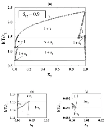
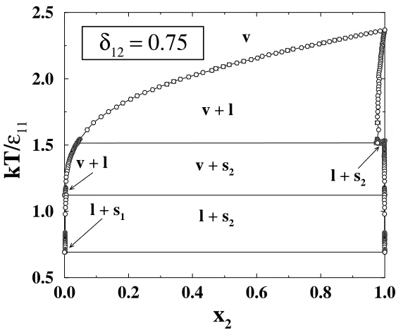
Chapter 3 explores the effect of the binary interaction parameter, δ12, on the

complete phase behavior of a mixture. We present complete phase diagrams for

(23)

ra-tio 11/22 = 0.45, and binary interaction parameters δ12 = 1.0,0.9,and 0.75, at

reduced pressure, P∗ ₌ P σ₁₁3/11 = 0.05. For the mixture with δ12 = 1 we ﬁnd a

completely miscible vapor-liquid coexistence region with a eutectic solid-liquid

co-existence region. These two regions are separated by a completely miscible liquid

phase. For the mixtures withδ12 <1 we ﬁnd that the vapor-liquid and solid-liquid

coexistence regions interfere. This interference results in a vapor-solid coexistence

region bounded above and below by solid-liquid-vapor coexistence lines. We also

ﬁnd that the mixtures withδ12 <1 have a region of liquid-liquid immiscibility that

is metastable with respect to the solid-ﬂuid phase equilibria.

Chapter 4 explores the effect of pressure on the complete phase behavior of

a mixture. We present complete,T −x phase diagrams for binary Lennard-Jones mixtures with diameter ratio σ11/σ22 = 0.85 and 11/22 = 1.6 at reduced

pres-suresP∗= 0.002, 0.01, 0.025, 0.05, and 0.1. We ﬁnd that as pressure increases, the vapor-liquid coexistence region ﬁrst shifts to higher temperatures and then begins

to disappear as the pressure approaches critical conditions. We summarize these

results on aP−T projection that identiﬁes the three-phase coexistence features of the mixture (solid-liquid-vapor and solid-solid-liquid) in addition to the pure

compo-nent vapor-liquid, solid-liquid, and vapor-solid coexistence curves. We then present

three moreP −T projections for mixtures with σ11/σ22 = 0.85, 0.9, and 0.95, and

11/22 = 0.45 so that we can observe how the features on these phase diagrams

change with variations in diameter ratio σ11/σ22 and well-depth ratio 11/22. We

(24)

solid-liquid-vapor coexistence pressures decreases and the locus of solid(1)-solid(2)-liquid

tem-peratures shifts from temtem-peratures above the solid-liquid temperature of pure

com-ponent 1 to temperatures below the solid-liquid coexistence temperature of pure

component 1. We ﬁnd that as well-depth ratio decreases the coexistence curves for

pure component 2 shift from temperatures and pressures below those of pure

com-ponent 1 to temperatures and pressures above those of pure comcom-ponent 1 and that

the maximum in the locus of solid-liquid-vapor coexistence pressures increases.

Chapter 5 is a study of a binary Lennard-Jones mixture with the following

pa-rameters: σ11 = σ22 = 1.0, σ12 = 0.85, 11 = 1.0, 12 = 0.82, and 22 = 1.2. We

calculate completeT−x phase diagrams for this mixture at reduced pressuresP∗

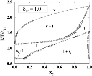
= 0.007, 0.05, and 0.1. Using these results we construct aP −T projection showing the three-phase loci for heteroazeotropes (l1l2v), monotectics (l1l2s), and eutectics

(s1s2l). Fluid phase coexistence points for this mixture have also been calculated

by Canongia Lopes10 _{using Gibbs ensemble Monte Carlo. They found a locus of}

heteroazeotrope temperatures that coincides with our heteroazeotrope locus but

disappears above T∗ = 1.1 and below T∗ = 0.9. Canongia Lopes interpreted this disappearance of liquid-liquid immiscibility aboveT∗ =1.1 and belowT∗= 0.9 as evidence for the presence of upper and lower critical endpoints, respectively. Based

on these inferred upper and lower critical endpoints, Canongia Lopes concluded that

this mixture displays Type VI behavior (closed-loop liquid-liquid immiscibility). In

our calculations we did not observe any evidence of Type VI phase behavior and

(25)

For completeness, an earlier study on solid-liquid equilibria for binary

Lennard-Jones mixtures has been included in Appendix A. This work was defended as part

of my Master of Science research in October, 1998. To our knowledge, these were

the ﬁrst direct simulations of solid-liquid equilibrium in binary Lennard-Jones

mix-tures. We calculated solid-liquid phase diagrams for binary Lennard-Jones mixtures

with diameter ratios ranging from 0.85 to 1 and attractive well-depth ratios ranging

from 0.45 to 1.6, at a reduced pressureP∗₌0.002. In a test of the cell theory pre-dictions11_{for model argon-methane, argon-krypton, and krypton-methane systems,}

we found that cell theory can qualitatively predict the shape of phase diagrams

for Lennard-Jones mixtures. Comparison of our simulation results for the

argon-krypton Lennard-Jones system with hard sphere results at the same diameter ratio

indicated that the presence of attractive interactions can change the type of phase

diagram observed from azeotrope (hard sphere) to solid solution (Lennard-Jones).

This suggested that attractive interactions are an important factor in determining

the type of solid-liquid phase behavior observed and prompted a more thorough

investigation of the effect of variations in well-depth ratio on solid-liquid phase

dia-grams. We simulated 56 binary Lennard-Jones mixtures over the range of parameters

listed above to determine how solid-liquid phase diagrams change as a function of

diameter ratio and well-depth ratio. We found that for well-depth ratios of unity

(equal attractions among species) phase behavior indicative of azeotropes and

eu-tectics is observed for diameter ratios ranging from 0.85 to 1. We then varied the

(26)

transitions from azeotrope to solid solution, from azeotrope to eutectic, and from

solid solution to simple peritectic. Using our simulation results, we were able to

map out the boundaries separating regimes of solid solution, azeotrope and

eutec-tic solid-liquid phase behavior in the space spanned by the Lennard-Jones diameter

ratio and well-depth ratios.

Chapters 2 through 5 and AppendixA have been adapted from the following

publications:

Chapter 2 M. H. Lamm and C. K. Hall, “Molecular simulation of complete phase diagrams for binary mixtures”,AIChE Journal, (submitted, 2000).

Chapter 3 M. H. Lamm and C. K. Hall, “Monte Carlo simulations of complete phase diagrams for binary Lennard-Jones mixtures”,Fluid Phase Equilibria, (accepted,

2000).

Chapter 4 M. H. Lamm and C. K. Hall, “The effect of pressure on complete phase behavior for binary mixtures”,Journal of Chemical Physics, (to be submitted).

Chapter 5 M. R. Hitchcock and C. K. Hall, “Complete phase diagrams for binary mix-tures via Gibbs-Duhem integration”,Proceedings of the Foundations of

Molecu-lar Modeling and Simulation Conference, Keystone, CO, 2000, (accepted, 2000).

(27)

1.2 References

[1] S. C. Stinson, Chemical and Engineering News,71, 38+ (1993).

[4] C. R. Bayley and N. A. Vaidya. inChirality in Industryedited by A. N. CollinsG. N.

Sheldrake and J. Crosby, pages 69–77, (1992).

[5] J. Jacques, A. Collet, and S. H. Wilen,Enantiomers, Racemates, and Resolutions.

(Krieger Publishing Company, Malabar, Florida, 1981).

[6] J. Crosby, Tetrahedron,47(27), 4789–4846 (1991).

[7] F. J. J. Leusen, J. H. Noordik, and H. R. Karfunkel, Tetrahedron, 49(24), 5377– 5396 (1993).

[8] D. A. Kofke, Journal of Chemical Physics,98(5), 4149–4162 (1993).

[9] R. Agrawal and D. A. Kofke, Molecular Physics,85(1), 43–59 (1995).

[10] J. N. C. Lopes, Molecular Physics,96(11), 1649–1658 (1999).

(28)

Chapter

2

Molecular simulation of complete phase

diagrams for binary mixtures

2.1 Introduction

Knowledge of the phase behavior of mixtures is crucial to the successful design

and operation of countless processes encountered in chemical engineering practice.

Design engineers need to know, for example, whether they will encounter

precipi-tates in pipelines, liquid-liquid separation in a distillation column, or cosolvency in a

supercritical ﬂuid extraction column. Although the phase equilibrium of a mixture

can, in principle, be measured at any condition of interest, ultimately, one would

like to be able to predict mixture phase behavior based solely upon knowledge of

the components’ molecular architecture and intermolecular forces.

The prediction of phase equilibria for mixtures has been the subject of

inten-sive investigation for decades. Two kinds of studies have been conducted: (1) those

aimed at developing accurate predictions of phase equilibria for speciﬁc substances

(29)

at providing general intuition about the overall topography of phase diagrams for

broad classes of substances, with particular focus on how intermolecular forces

impact phase diagram shape. The latter type of study is exempliﬁed by the work

of van Konynenburg and Scott1,2_{, who analyzed how the types of phase diagrams}

predicted by the van der Waals equation of state for binary mixtures depend on

the values of the van der Waals size and energy parameters. Remarkably, the

sim-ple van der Waals equation of state was found to exhibit ﬁve of the six types of

ﬂuid phase behavior observed experimentally. This landmark study has been

fol-lowed by similar analyses for other equations of state, such as the Redlich-Kwong3_,

the Carnahan-Starling-Redlich-Kwong4, the Guggenheim5, and the Ree6equations of

state.

Most of the research aimed at understanding how intermolecular interactions

affect phase behavior has focused exclusively on ﬂuid phase equilibria. However

in real systems solid phases form and often interrupt the complexphase behavior

exhibited by ﬂuids7,8_{. Phenomenological descriptions of complete phase behavior}

(i.e., showing equilibrium between vapor, liquid, and solid phases) have been given

by Luks9_{, Peters} _{et al.}10_{, and Valyashko}11,12_{. Luks and Peters} _{et al.} _{describe four}

types of complete phase diagrams observed for binary mixtures of solvent (methane,

ethane, carbon dioxide) and a homologous series of solutes (n-alkanes). Valyashko proposes a classiﬁcation scheme for twelve types of complete diagrams. Eight of

these types result from the analysis of experimental data for water-inorganic salt

(30)

topological transformation, which involves making educated guesses about the

tran-sitions in topography between the eight known types. This method is based on the

idea that there are continuous transitions between all types of phase behavior13_.

A quantitative description of complete phase behavior has been given by Luks

and coworkers14,15_{. Garcia and Luks}14 _{calculate the solid-liquid-vapor locus for}

bi-nary mixtures of solvent and a homologous series of solutes using the van der Waals

equation of state for the ﬂuid phase and a simple fugacity model for the solid phase.

This work was extended by Labadie et al.15 _{who calculated the ﬂuid phase critical}

loci for these mixtures, offering a picture of how the multiphase topography

pro-gresses with changes in the solute properties. They found examples of solid-ﬂuid

phase behavior in keeping with what has been observed in real systems, as well as

solid-ﬂuid phase behavior that has yet to be veriﬁed by experiment. As with any

analytical equation of state, there exists the possibility that the new topographies

are mathematical artifacts stemming from the approximations made in the

devel-opment of the equation of state. Nonetheless, the new possibilities for complete

phase behavior calculated by Luks and coworkers are intriguing and invite further

investigation.

The most accurate way to determine how molecular size, shape, and energy of

interaction inﬂuence phase equilibria is with molecular simulation, since molecular

simulations provide exact results for the model system being studied16_{. A signiﬁcant}

advance was made in the simulation of phase equilibria when Panagiotopoulos17,18

(31)

are simulated independently, yet are coupled thermodynamically in order to satisfy

the criteria of phase equilibrium: equal temperatures, pressures, and species

chem-ical potentials. These conditions are satisﬁed by simulating each phase at the same

temperature and pressure, and performing particle transfers between the phases to

maintain chemical potential equality.

Although the Gibbs ensemble method has been widely adopted for studying

ﬂuid phase equilibria, it is not an efﬁcient method for studying solid phase

equi-libria because a large number of successful particle transfers between each phase

are required for chemical potential equilibration. Inspired by the Gibbs ensemble

method, Kofke19,20 introduced the Gibbs-Duhem integration technique for direct

simulation of phase equilibria. As in the Gibbs ensemble method, two or more

co-existing phases are simulated independently at the same temperature and pressure.

However, instead of using particle transfers, the chemical potential equality among

each phase is maintained by integrating along the Clapeyron differential equation

for coexistence during the simulations. Eliminating the need for particle transfers

between phases makes the Gibbs-Duhem integration method well-suited for

calcu-lating phase equilibrium for cases in which one of the phases is a solid. The method

requires an initial coexistence condition to begin the integration of the Clapeyron

equation; this initial condition can be obtained from simulation data (e.g., a Gibbs

ensemble simulation or a previous Gibbs-Duhem integration), a reliable theory, or

experimental data.

(32)

behavior has been the Lennard-Jones ﬂuid, the quintessential model of a system

containing spherically symmetric molecules. The Lennard-Jones intermolecular

po-tential is given by

uij(r )=4ij

_σ

ij r

12

−

_σ

ij r

6

, (2.1)

where uij is the potential energy of interaction between particles iand j, r is the

distance between particles i and j, ij is the Lennard-Jones attractive well-depth,

andσij is the Lennard-Jones diameter. Simulations of the ﬂuid phase behavior for

Lennard-Jones mixtures have proven useful for testing theories21–23 as well as for

developing general intuition regarding the inﬂuence of molecular size and

inter-molecular interactions on phase behavior24–28_.

In AppendixA we used the Gibbs-Duhem integration method combined with

semigrand canonical Monte Carlo simulations to calculate solid-liquid phase

dia-grams for binary Lennard-Jones mixtures over a range of diameter ratiosσ11/σ22=

0.85−1.0 and well-depth ratios11/22=0.45−1.6. The cross-species interaction

pa-rameters were calculated using the Lorentz-Berthelot30 _{combining rules. We found}

that for well-depth ratios of unity (equal attractions among species), phase behavior

indicative of eutectics and solid solutions with minimum melting points is observed

for diameter ratios ranging from 0.85 to 1. We then varied the well-depth ratio of

the mixtures at several constant diameter ratios and observed transitions from solid

solution to solid solution with a minimum melting point, from solid solution with a

minimum melting point to eutectic, and from solid solution to peritectic. Using our

(33)

solid solution, solid solution with a minimum melting point, eutectic, and peritectic

solid-liquid phase behavior in the space spanned by the Lennard-Jones diameter and

well-depth ratios.

More recently, we have demonstrated that the Gibbs-Duhem integration method

can be used to calculate complete phase diagrams31,32_{where by “complete” we mean}

containing all possible phases: solid, liquid, and vapor. Prior to that, complete

phase diagrams for symmetric (equal diameters, σ11 = σ22; equal attractive

well-depths, 11 = 22) Lennard-Jones mixtures were calculated by Vlot et al.33 using

a combination of molecular simulation and semiempirical models. In their work,

Monte Carlo simulations were conducted for each phase at selected state points

to determine the excess free energy as a function of composition. The resulting

free energy versus composition data was ﬁt with a two-parameter Redlich-Kister

polynomial and the convexenvelope construction method was used to determine the

phase diagram. In comparison to this somewhat indirect method, the Gibbs-Duhem

integration method can be applied to the calculation of complete phase diagrams

with relative ease.

Our objective in this chapter is to explore the effect of both molecular size and

intermolecular attractions on the complete phase behavior of a mixture. We calculate

complete phase diagrams for binary Lennard-Jones mixtures with diameter ratios

ranging from 0.85 – 0.95 and attractive well-depth ratios ranging from 0.625 – 1.6,

at a reduced pressureP∗ ≡ P σ₁₁3/11 = 0.002, which is equivalent to atmospheric

(34)

Lorentz-Berthelot combining rules. We restrict ourselves to diameter ratios ranging

from 0.85 to 0.95 because in this region the only kind of solid phase that can form is

a substitutionally disordered fcc solid solution (the two species pack onto the same

fcc crystalline lattice and can substitute for one another in any order on the lattice).

(At diameter ratios less than 0.85, the calculation is more complexbecause several

ordered crystalline phases are possible, necessitating the calculation of each phase’s

the free energy to determine the most stable crystalline structure.) Vapor-liquid,

solid-liquid, and solid-vapor lines are calculated for each mixture by integrating the

Clapeyron differential equation for binary mixture phase equilibria at constant

pres-sure. The initial conditions for the integrations are the vapor-liquid and solid-liquid

coexistence data for a single component Lennard-Jones system at P∗ = 0.002 ob-tained via Gibbs-Duhem integration19,34_{. The properties of each phase at subsequent}

integration points are determined by semigrand canonical Monte Carlo simulations

(constant temperature, pressure, total number of molecules, and fugacity fraction)

on the vapor, liquid, and solid phases.

Highlights of our results are the following. We ﬁnd that for well-depth ratios of

unity (equal attractions among species) there is no interference between the

vapor-liquid and solid-vapor-liquid coexistence regions. As the well-depth ratio increases or

decreases from unity, the vapor-liquid and solid-liquid phase envelopes widen and

interfere with each other leading to a solid-vapor coexistence region. For all

well-depth ratios and a diameter ratio of 0.95, the solid-liquid lines have a shape

(35)

the diameter ratio decreases the solid-liquid lines fall to lower temperatures until

they eventually drop below the solid-solid coexistence region, resulting in either a

eutectic or peritectic three-phase line.

The remainder of the chapter is organized as follows. In the next section we

outline the Gibbs-Duhem integration method and describe how we applied the

pro-cedure to the calculation of mixture phase behavior for solid, liquid, and vapor

phases. We then present the complete phase diagrams, followed by a discussion of

the results. Finally, we conclude with a brief summary and further discussion.

2.2 Gibbs-Duhem integration

In this section we describe how we calculated phase equilibria for binary

Lennard-Jones mixtures using the Gibbs-Duhem integration method. We begin by

presenting a brief review of the Gibbs-Duhem integration method. We then discuss

our procedures for determining an initial coexistence condition and integrating the

Clapeyron equation. Finally, we describe the details of the semigrand ensemble

sim-ulations used throughout the integration procedure to determine the properties of

each of the coexisting phases.

The coexistence lines were calculated using Gibbs-Duhem integration20,35_{. In}

this method, phase coexistence is determined by numerically integrating the

Clapey-ron differential equation appropriate to the system of interest. ClapeyClapey-ron equations

describe how ﬁeld variables (variables that must be equal among coexisting phases)

(36)

between two phases (αandγ) of a binary mixture containing components 1 and 2 at constant pressure is

dβ dξ2 =

(x₂α−x₂γ) ξ2(1−ξ2)(hα−hγ)

, (2.2)

whereβis the reciprocal temperature, 1/kT, withkthe Boltzmann constant and T

the absolute temperature,ξ2is the fugacity fraction of species 2,ξ2≡f2/ fi, with

fi, the fugacity of speciesiin solution,x2is the mole fraction of species 2, andhis

the molar enthalpy. The right-hand side of Eq. (2.2) can be integrated numerically to

ﬁnd an equation forβas a function of ξ2if we have an initial condition describing

the temperature, fugacity fraction, enthalpies and compositions at one coexistence

point.

2.2.1 Initial condition

An initial coexistence condition is necessary to begin a Gibbs-Duhem

integra-tion calculaintegra-tion for phase equilibrium in a binary mixture. A convenient choice for

the initial coexistence condition is the vapor-liquid or solid-liquid equilibrium

con-dition for either of the pure Lennard-Jones components. Here, we used literature

data obtained via Gibbs-Duhem integration for the vapor-liquid19_{and solid-liquid}34

coexistence conditions. The integrand in Eq. (2.2) is undeﬁned for pure components

(ξ2=0, x2=0 andξ2=1, x2=1) but it can be estimated using the limiting case of

inﬁnite dilution. Here we follow Mehta and Kofke36_{, who used the inﬁnite dilution}

case to start their Gibbs-Duhem integration calculations of vapor-liquid equilibria in

(37)

The limiting value of the integrand whenx2approaches zero,(dβ/dξ2)x2=0, can be estimated by supposing that the real mixture displays ideal solution behavior

at the limit of inﬁnite dilution of species 2. With this assumption, the abundant

component (species 1) in the ideal solution follows the Lewis Randall rule

f1=x1f1, (2.3)

while the dilute component (species 2) obeys Henry’s law

f2=x2H2, (2.4)

where f1 is the fugacity of pure component 1 at the temperature and pressure of

the mixture, andH2 is the Henry’s law constant for species 2. Letting x1 →1 and

x2 → 0, the fugacity fraction of species 2 becomes, ξ2 = x2H2/f1. After making

these substitutions into Eq. (2.2) and rearranging terms29 we get

dβ dξ2

x2=0

= f1(1/H2α−1/H

γ

2)

(hl₋_hs₎ . (2.5)

This gives us an estimate for the integrand at the initial condition of ξ2 = 0 and

coexistence (e.g., solid-liquid, vapor-liquid) temperature, T1, of pure species 1. A

similar formula can be derived in the limit of inﬁnite dilution of species 1.

We can calculate all of the quantities on the right-hand side of Eq. (2.5) with

(38)

u+P v NPT, where uis the conﬁgurational energy of the system and the brackets, NPT, denote an NPT ensemble average. The quantityf1/H2can be calculated from36

f1

H2 =

exp(−β∆u1→2) NPT (2.6)

where ∆u1→2 is the exchange energy associated with switching a particle from

species 1 to 2. The exchange energy, ∆u1→2, can be obtained by conducting trial

identity switches during the simulation; these involve randomly selecting a particle

and calculating the energy that would result if we were to switch the particle from

species 1 to species 2. This is done without actually changing the particle’s identity.

2.2.2 Integration

Once we have an initial coexistence condition, the Gibbs-Duhem integration

pro-cedure may be performed over the entire range of fugacity fractions,ξ2= 0 toξ2 =

1, using a predictor-corrector algorithm to integrate Eq. (2.2). Starting at the initial

condition, β0, (ξ2)0, we step to the next fugacity fraction, (ξ2)1, and estimate the

associated reciprocal temperature,β1, using the trapezoid-rule predictor formula

β(₁0)=β0+[(ξ2)1−(ξ2)0] F (β0, (ξ2)0), (2.7)

where the superscript “0” indicates that β(₁0) (a predicted value) is our zeroth iter-ation attempt at ﬁnding the reciprocal temperatureβ1and F is the right-hand side

(39)

fugacity fraction (ξ2)1, two semigrand canonical (NPTξ2) Monte Carlo simulations

(one for the αphase and one for the γ phase) are conducted in order to calculate the enthalpies and mole fractions of each phase at the new state point. (Details of

the NPTξ2simulations will be given in Section 2.2.3.)

After the enthalpies and mole fractions at the new state point are calculated we

reﬁne the estimate forβ1at(ξ2)1by performing a loop of corrector iterations until

β1converges within an acceptable tolerance. The general form of the trapezoid-rule

corrector for this loop is given by

β(i₁+1)=β0+

[(ξ2)1−(ξ2)0]

2

F₁(i)(β(i)₁ , (ξ2)1)+F0(β0, (ξ2)0) , (2.8)

where the superscripts(i)and (i₊1) denote the iterations of the corrector, the sub-scripts “0” and “1” denote the initial and current state point, respectively, andF₁(i)

is calculated from simulation averages of the enthalpies and mole fractions during

the ith _{iteration of the corrector at} _β(i)

1 and (ξ2)1. After β1 converges a

produc-tion segment of simulaproduc-tions are run to obtain the ﬁnal average enthalpies and mole

fractions for the coexistence point. Once the production runs are completed, the

fugacity fraction is incremented and the predictor-corrector algorithm described

above is repeated to obtain the next state point,β2,(ξ2)2.

Higher order predictor-corrector equations are used as we obtain more state

points. The midpoint predictor-corrector is used once two state points are known,

(40)

β(i_n₊+₁1)=βn−1+

[(ξ2)n+1−(ξ2)n]

3

F_n(i)₊₁+4Fn+Fn−1 , (2.10)

and the modiﬁed Adams predictor-corrector37 _{is used once three or more state}

points are known,

β(_n0₊)₁=βn+

[(ξ2)n+1−(ξ2)n]

24 [55Fn−59Fn−1+37Fn−2−9Fn−3] , (2.11)

β(i_n₊+₁1)=βn+

[(ξ2)n+1−(ξ2)n]

24

9F_n(i)₊₁+19Fn−5Fn−1+Fn−2 . (2.12)

In these sets of equations the predictor is listed ﬁrst and the corrector second. The

subscripts denote the coexistence state points with(n₊1) being the current state point and the superscripts denote the iterations of the corrector for the current

coexistence state point. By repeating the predictor-corrector algorithm fromξ2=0

toξ2=1 we can map out the entire temperature versus composition phase diagram.

In some of the mixtures, we encountered interference between two different

two-phase coexistence regions e.g., the vapor-liquid and solid-liquid coexistence

curves overlapped, resulting in a three-phase solid-liquid-vapor coexistence line. In

this case, two Gibbs-Duhem integrations were conducted, the ﬁrst starting from the

vapor-liquid coexistence temperature for one of the pure components and the

sec-ond starting from the solid-liquid coexistence temperature for the same pure

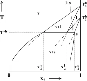
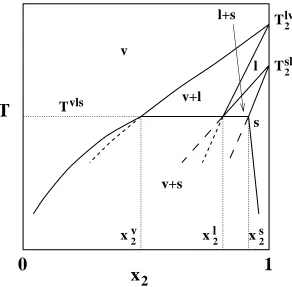
com-ponent. For example, in Figure 2.1 vapor-liquid and solid-liquid coexistence curves

can be calculated starting from the vapor-liquid and solid-liquid coexistence

temper-atures (T₂lv andT₂ls, respectively) of pure component 2. At someξ2(unknown at the

(41)

set of coexistence curves will cross, thus, determining the temperature, fugacity

frac-tion, and coexistence compositions of the three coexisting phases: vapor, liquid, and

solid. In Figure 2.1 the liquid lines cross atTvls _and_xl

2. BelowTvls the inner

vapor-liquid and solid-vapor-liquid coexistence curves (shown by short-dashed and long-dashed

lines, respectively) are metastable with respect to the outer vapor-solid coexistence

curves, according to the boundary curvature rule38,39_{, which states that the}

bound-aries of one-phase regions must meet at a three-phase line with curvatures such

that the boundaries extrapolate into the two-phase coexistence regions.. The

vapor-solid coexistence curve is determined by a Gibbs-Duhem integration starting from

Tvls at x₂v andx₂s. Other types of three-phase coexistence lines (heteroazeotropes, eutectics, etc.) can be determined in a similar manner.

2.2.3 Simulations

The enthalpies and mole fractions needed as input to the integration of Eq. (2.2)

are obtained from semigrand canonical (constant NPTξ2) Monte Carlo computer

sim-ulations40_{. In this work, all simulations were run with a system size of 500 particles}

at a reduced pressure P∗ = 0.002. The temperature and fugacity fraction were ﬁxed at the values speciﬁed by the Gibbs-Duhem integration predictor-corrector

al-gorithm. There are three types of Monte Carlo trial moves in semigrand canonical

simulations: particle displacements, volume change moves, and particle identity

ex-changes. The particle displacements and volume change moves are conducted just

(42)

a particle is selected at random and given a trial species identity switch, which is

accepted according to the ratio of the species fugacity fractions,ξ1andξ2. The

over-all acceptance probability36 _{for the moves in the NPT}_ξ

2ensemble is min[1,exp(Λ)]

where

Λ= −β(Utrial−Uold)−βP (Vtrial−Vold)+NlnV

trial

Vold +mln

ξ2

1₋ξ2

. (2.13)

In Eq. (2.13),Utrial _and_Uold_{, and}_Vtrial _and_Vold_{, are the conﬁgurational energies and}

volumes of the trial and existing states, respectively, m _{= +}1 if the trial identity switch is from species 1 to 2, andm= −1 if the trial identity switch is from species 2 to 1. In NPTξ2simulations the choice of the type of Monte Carlo move is made

ran-domly but weighted such that the ratio of attempted moves is 1 volume change toN

particle displacements toNidentity switches. The length of the simulation is given in cycles, where one cycle represents 1 volume change attempt,Ndisplacement at-tempts, andN identity switch attempts. In our work, a typical NPTξ2simulation is

equilibrated for 3000 cycles and then followed by a production run of 5000 cycles

to compute the average enthalpy and mole fraction. The only difference between

ﬂuid and solid phase simulations is that to maintain an fcc crystalline structure in

the solid phase simulations we impose a single occupancy constraint41,42_{on the trial}

displacements of particles in the solid,i.e., any displacements that put the particle

outside its lattice cell are rejected.

Other details of the NPTξ2 simulations are as follows. The simulation volume

(43)

Lennard-Jones potential model. We determine the cross-species interaction

param-eters (σ12, 12) by using the Lorentz-Berthelot30mixing rulesσ12=(σ11+σ22)/2 and

12 =√1122. The potential interactions are truncated at a cutoff radius of half the

boxlength. To compensate for this truncation, a long range correction is applied

to the energy calculations during the simulation by assuming a uniform density

distribution beyond the cutoff radius16_.

2.3 Results and Discussion

In this section, we present the results of our Gibbs-Duhem integration

calcu-lations of complete phase behavior for binary Lennard-Jones mixtures. All of the

phase diagrams were calculated at reduced pressure,P∗_≡P σ₁₁3/11=0.002, which

is equivalent to atmospheric pressure for argon. We calculated nine phase diagrams

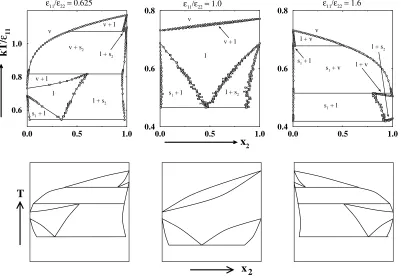
for diameter ratios σ11/σ22 = 0.85, 0.9, and 0.95, and well-depth ratios 11/22 =

0.625, 1.0, and 1.6. For these diameter ratios, the solid phase has a substitutionally

disordered fcc crystalline structure.

In the ﬁrst series, we calculated phase diagrams for binary mixtures with

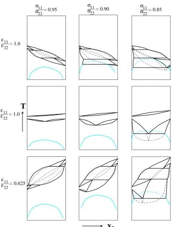
σ11/σ22= 0.95 and11/22= 0.625, 1.0, and 1.6. Figure 2.2 shows the

temperature-composition phase diagrams obtained via Gibbs-Duhem integration (row 1) along

with not-to-scale schematic diagrams (row 2) drawn to illustrate the smaller features

of the actual phase diagram more clearly. On the phase diagram for11/22=0.625,

vapor-liquid coexistence lines originate from pure component 2 (x2 = 1, T∗ ≡

(44)

Solid-liquid coexistence lines originate from pure component 2 (x2=1, T∗=1.099)

and decrease in temperature with decreasing fugacity fractionξ2. The liquid-vapor

and solid-liquid curves meet at T∗ = 1.093 and form a three-phase, solid-liquid-vapor equilibrium line. Solid-solid-liquid-vapor coexistence lines originate from this three-phase

line and decrease in temperature with decreasing fugacity fractionξ2. Vapor-liquid

curves originate from pure component 1 (x2 = 0, T∗ = 0.732) and increase in

temperature with increasing fugacity fractionξ2. The vapor-liquid and vapor-solid

curves meet at T∗ = 0.745 and form a three-phase, vapor-liquid-solid equilibrium line. Liquid-solid coexistence lines originate from this three-phase line and decrease

in temperature with decreasing fugacity fractionξ2until they reach the solid-liquid

coexistence temperature for pure component 1 (x2 = 0, T∗ = 0.687). A miscible

solid phase exists below the solid-liquid curves.

On the phase diagram for11/22=1.0, vapor-liquid coexistence lines originate

from pure component 2 (x2=1, T∗=0.742) and decrease in temperature with

de-creasing fugacity fraction until they reach the vapor-liquid coexistence temperature

for pure component 1 (x2=0, T∗=0.732). A miscible liquid phase exists below the

vapor-liquid curves. Solid-liquid coexistence lines originate from pure component 2

(x2=1, T∗=0.687) and decrease in temperature with decreasing fugacity fraction

ξ2to a minimum melting point (x2=0.508, T∗=0.666). The solid-liquid lines then

increase in temperature with decreasing fugacity fraction ξ2 until they reach the

solid-liquid coexistence temperature for pure component 1 (x2=0, T∗ =0.687). A

(45)

On the phase diagram for11/22=1.6, liquid-vapor coexistence lines originate

from pure component 1 (x2 = 0, T∗ = 0.732) and decrease in temperature with

increasing fugacity fraction ξ2. Solid-liquid coexistence lines originate from pure

component 1 (x2 = 0, T∗ = 0.687) and decrease in temperature with increasing

fugacity fractionξ2. The liquid-vapor and solid-liquid curves meet atT∗=0.681 and

form a three-phase, solid-liquid-vapor equilibrium line. Solid-vapor coexistence lines

originate from this three-phase line and decrease in temperature with increasing

fugacity fractionξ2. Liquid-vapor coexistence lines originate from pure component

2 (x2=1, T∗=0.485) and increase in temperature with decreasing fugacity fraction

ξ2. The liquid-vapor and solid-vapor curves meet at T∗ = 0.495 and form another

three-phase, solid-liquid-vapor equilibrium line. Solid-liquid lines originate from

this three-phase line and decrease in temperature with increasing fugacity fraction

ξ2 until they reach the solid-liquid coexistence temperature for pure component 2

(x2=0, T∗=0.429). A miscible solid phase exists below the solid-liquid curves.

In the second series, we calculated phase diagrams for binary mixtures with

σ11/σ22 = 0.9 and11/22 = 0.625, 1.0, and 1.6. Figure 2.3 shows the

temperature-composition phase diagrams obtained via Gibbs-Duhem integration (row 1) along

with not-to-scale schematic diagrams (row 2) drawn to illustrate the smaller features

of the actual phase diagram more clearly. On the phase diagram for11/22=0.625,

vapor-liquid coexistence lines originate from pure component 2 (x2=1, T∗=1.157)

and decrease in temperature with decreasing fugacity fractionξ2. Liquidsolid coex

(46)

temperature with decreasing fugacity fraction ξ2. The vapor-liquid and liquid-solid

curves meet at T∗ ₌ 1.086 and form a three-phase, vapor-liquid-solid equilibrium line. Vapor-solid coexistence lines originate from this three-phase line and decrease

in temperature with decreasing fugacity fraction. Vapor-liquid curves originate from

pure component 1 (x2=0, T∗=0.732) and increase in temperature with increasing

fugacity fraction. The vapor-liquid and vapor-solid curves meet atT∗= 0.770 and form another three-phase, vapor-liquid-solid equilibrium line. Liquid-solid

coexis-tence lines originate from this three-phase line and decrease in temperature with

de-creasing fugacity fraction ξ2to a minimum melting point (x2= 0.195, T∗=0.665).

The solid-liquid lines then increase in temperature with decreasing fugacity fraction

ξ2 until they reach the solid-liquid coexistence temperature for pure component 1

(x2=0, T∗=0.687). A miscible solid phase exists below the solid-liquid curves.

On the phase diagram for11/22=1.0, vapor-liquid coexistence lines originate

from pure component 2 (x2=1, T∗=0.753) and decrease in temperature with

de-creasing fugacity fraction until they reach the vapor-liquid coexistence temperature

for pure component 1 (x2=0, T∗=0.732). A miscible liquid phase exists below the

vapor-liquid curves. Solid-liquid coexistence lines originate from pure component 2

(x2=1, T∗=0.687) and decrease in temperature with decreasing fugacity fraction

ξ2to a minimum melting point (x2=0.440, T∗=0.593). The solid-liquid lines then

increase in temperature with decreasing fugacity fraction ξ2 until they reach the

solid-liquid coexistence temperature for pure component 1 (x2=0, T∗ =0.687). A

(47)

On the phase diagram with11/22 = 1.6, liquid-vapor coexistence lines

origi-nate from pure component 1 (x2=0, T∗=0.732) and decrease in temperature with

increasing fugacity fraction. Solid(1)-liquid coexistence lines originate from pure

component 1 (x2=0, T∗ =0.687) and decrease in temperature with increasing

fu-gacity fractionξ2. The liquid-vapor and solid(1)-liquid curves meet at T∗ = 0.679

and form a three-phase, solid(1)-liquid-vapor equilibrium line. Solid(1)-vapor

coex-istence lines originate from this three-phase line and decrease in temperature with

increasing fugacity fraction ξ2. Liquid-vapor coexistence lines originate from pure

component 2 (x2=1, T∗ =0.494) and increase in temperature with decreasing

fu-gacity fractionξ2. The liquid-vapor and solid(1)-vapor curves meet at T∗ = 0.505

and form another three-phase, solid(1)-liquid-vapor equilibrium line. Solid(1)-liquid

lines originate from this three-phase line and decrease in temperature with

increas-ing fugacity fractionξ2. Liquid-solid(2) coexistence lines originate from pure

com-ponent 2 (x2=1, T∗=0.429) and increase in temperature with decreasing fugacity

fraction ξ2. The solid(1)-liquid and liquid-solid(2) curves meet at T∗ = 0.437 and

form a three phase, solid(1)-solid(2)-liquid equilibrium line. This line is also known

as a peritectic. Below this temperature (not shown in Figure 2.3) solid(1) and solid(2)

are in equilibrium. Although Gibbs-Duhem integration method we employ can be

readily applied to solid-solid equilibria we have not calculated solid(1)-solid(2)

coex-istence lines in this work since they are not necessary for classifying the solid-liquid

behavior.

Monte Carlo Simulations of Complete Phase Equilibria for Binary Mixtures

EQUILIBRIA FOR BINARY MIXTURES

Biography

Acknowledgements

Table of Contents

List of Tables

List of Figures

Chapter

1

Introduction

1.1

Overview

1.2

References

Chapter

2

Molecular simulation of complete phase

diagrams for binary mixtures

2.1

Introduction

2.2

Gibbs-Duhem integration

2.3

Results and Discussion