Bat Algorithm for Solving Dynamic Economic Emission Dispatch Problem

Bat Algorithm for Solving Dynamic Economic

Emission Dispatch Problem

M. Iqbal Arsyad1, Bonar Sirait2, Hardiansyah Hardiansyah3

1, 2, 3

Department of Electrical Engineering, University of Tanjungpura, Pontianak 78124, Indonesia

Abstract

This paper proposes a new meta-heuristic search algorithm, called Bat Algorithm (BA). Bat algorithm is an optimization technique motivated by the echolocation behavior of natural bats in finding their foods. The proposed algorithm is presented to solve the dynamic economic emission dispatch (DEED) problem. As emission minimization is conflicting with minimum cost of generation, the DEED problem becomes a multi-objective optimization problem with conflicting objectives. The proposed algorithm is validated on 5-unit generation system for a 24 h time interval. The results proved the efficiency of the proposed method when compared with the other optimization algorithms reported in the literature.

Keywords: Bat algorithm, dynamic economic emission dispatch, prohibited operating zones, non-smooth cost function.

1. Introduction

The main objective of the dynamic economic dispatch (DED) problem of a power plant is to schedule generator unit outputs that are committed to meeting predicted load demand with minimum operating cost, while satisfying all system equality and inequality constraints. Hence, the DED problem is a very limited large-scale nonlinear optimization problem [1, 2]. The presence of the valve-point effect results ripples in the heat-rate curves so that the objective function becomes non-smooth, non-convex, and with multiple minima [3-5]. The fuel cost function with valve-point effects in the generating units is the accurate model of the DED problem [6, 7].

In recent years strategically utilizing available resources and achieving electricity at bargain prices without sacrificing social benefits is very important. The environmental pollution plays a major role as it had a major threat on the human society. Hence, it became compulsory to deliver electricity at a minimum cost as well as to maintain minimum level of emissions. Lowest emissions are considered as one of the objectives in combined economic and emission dispatch problems, along with cost economy. Atmospheric pollution due to release of gases such as nitrogen oxides (NOX), carbon

dioxide (CO2), and sulphur oxides (SOX) into atmosphere by fossil-fuel based electric power stations affects not only humans but also other forms of life such as birds, animals, plants and fish, while causes global warming too [8-11]. Generating units may have certain prohibited operating zones (POZs) due to faults in the machines themselves or instability concerns or the valve point effect. Hence, considering the effect of valve-points and POZs in generators’ cost function makes the economic dispatch a non-smooth and non-convex optimization problem [12].

The emission dispatch is a short-term alternative that should be optimized, besides fuel cost goals. Thus, DEED problem can be handled as a multi-objective optimization problem and requires only small modification to include emission. Therefore, the DEED problem can be converted into a single objective problem by linear combination of various objectives using different weights. The important characteristic of the weighted sum method is that different pareto-optimal solutions can be obtained by varying the weights [13]. In [14-16] the static economic dispatch problem with prohibited operating zones has been solved. A number of reported works has considered the prohibited operating zones in DED problem [17-20], however, the emission has not considered in these papers.

Latterly, a new meta-heuristic search algorithm, called Bat Algorithm (BA) [21], has been developed by Yang. In this paper, bat algorithm has been used to solve the DEED problem considering ramp rate limits, valve-point effects, prohibited operating zones, and transmission loss. The effectiveness and potential of the proposed approach is tested on a 5-unit generation system. The results obtained by the proposed BA technique are compared with other optimization results reported in literature.

2. Problem Formulation

www.ijiset.com

meet the power demand at minimum both operating cost and emission simultaneously.

The objective function of the DEED problem can be formulated as follow:

T t N i P E h w P F w

F _it

T t N i t i T t N i t i t i T , , 2 , 1 ; , , 2 , 1 for ) ( ) ( _, 1 1 , 2 1 1 , , 1   = = ∗ ∗ + ∗ =

∑∑

∑∑

= =

= = (1)

where FT is the total operating cost over the whole

dispatch period, T is the number of hours in the time horizon, N is the total number of generating units, w1 is

weighting factor for economic objective such that its value should be within the range 0 and 1, and w2is the weighting

factor for emission objective which is given by w2 = (1 -

w1), and hiis the price penalty factor. Fi,t(Pi,t) and Ei,t(Pi,t)

are the generation cost and the amount of emission for ith unit at time interval t , and Pi,t is the real power output of

generating ith unit at time period t.

The fuel cost of the ith thermal generating unit is expressed as the sum of a quadratic and a sinusoidal form with the valve-point effects taken into accout. Thus, the total generation cost is expressed as follows [12]:

(

)

(

)

       − × × + + + = sin ) ( , min , , 2 , , , t i i i i i t i i t i i t i t i P P f e c P b P a P

F (2)

where the constant ai, bi, and ci represents generator cost

coefficients and ei and fi represents valve-point effect

coefficients of the ith generating unit.

Utilization of thermal power plant consuming fossil fuel is with release of high amounts of NOX, they are strongly requested by the environmental protection agency to reduce their emissions. The NOX emission of the thermal power station having N generating units at interval t in the scheduling horizon is represented by the sum of quadratic and exponential functions of power generation of each unit. The emission due to ith thermal generating unit can be expressed as

(

)

(

i it i it i i i it

)

t i t

i P P P P

E 2 _{, ,}

, ,

,( )= α +β +γ +η expδ (3)

where αi,βi , γi , ηiand δi are emission coefficients of the

ith generating unit.

The minimization of the fuel cost and emission are subjected to the following equality and inequality constraints:

2.1 Power Balance Constraint

The total generated real power should be the same as total load demand plus the total line loss.

t L t D N i t

i P P

P _{, ,}

1

, = +

∑

=

(4)

where PD,t and PL,t are the demand and transmission loss

in MW at time interval t, respectively.

The transmission loss PL,t can be expressed by using B

matrix technique and is defined as:

t j ij N i N j t i t

L P B P

P _,

1 1 ,

,

∑∑

= =

= (5)

where Bij is the ij-th element of the loss coefficient square

matrix of size N.

2.2 Generation Limits

The real power output of each generators should lie between minimum and maximum limits.

max , , min

, it i

i

P

P

P

≤

≤

(6)

2.3 Ramp Rate Limits

The ramp-up and ramp-down constraints can be written as:

i t i t

i P UR

P, − ,−1 ≤ (7)

i t i t

i P DR

P,−1− , ≤ (8)

where Pi,t and Pi,t-1 are the present and previous real power

outputs, respectively. URi and DRi are the ramp-up and

ramp-down limits of ith unit (in units of MW/time period).

To consider the ramp rate limits and real power output limits constraint at the same times, therefore, equations (6), (7) and (8) can be rewritten as follows:

} ,

min{ }

,

max{Pi,min Pi,t−1−DRi ≤Pi,t ≤ Pi,max Pi,t−1+URi (9)

2.4 Prohibited Operating Zones

The possible operating zones of the generator can be described as follows [7, 15]:

      = ≤ ≤ = ≤ ≤ ≤ ≤ ∈ ₋ pz i t i u pz i i l k i t i u k i l i t i i t i n i P P P pz k P P P P P P P

i , 1,2, ,

, , 3 , 2 , max , , , , , 1 , 1 , , min , , 

 (10)

where l k i

P_, and

P

_iu_,k are the lower and upper boundary of prohibited operating zone of ith unit, respectively. Here, pziis the number of prohibited zones of ith unitand npz is

the number of units which have prohibited operating zones.

3. Bat Algorithm (BA)

Xin-She Yang in 2010 [21]. The algorithm mimics the echolocation behavior most prominent in bats. Bats send out streams of high-pitched sounds usually short and loud. These signals then bounce off nearby objects and send back echoes. The time delay between the emission and echo helps a bat navigate and hunt. This delay is used to interpret how far away an object is. Bats use frequencies ranging from 200 to 500 kHz. In the algorithm pulse rate ranges from 0 to 1 where 0 means no emissions and 1 means maximum emissions.

Natural bats are using the echolocation behavior in locating their foods. This echolocation characteristic is copied in the virtual Bat algorithm with the following assumptions [21]:

1. All the bats are following the echolocation mechanism and they could distinguish between prey and obstacle. 2. Each bat randomly with velocity viat position xi with a

fixed frequency fmin, varying wavelength λ and

loudness A0 while searching for prey. They adjust to

the frequency (or wavelength) of the transmitted pulse and set the pulse emission rate r∊ [0, 1], depending on the distance of the prey.

3. Although the loudness can vary in many ways, we assume that the loudness varies from a large (positive) A0 to a minimum constant value Amin.

3.1 Initialization of Bat Algorithm

Initial population is generated randomly for n number of bats. Each individual of the population consists of real valued vectors with d dimensions [21]. The following equation is used to generate the initial population:

x

_ij

=

x

_minj

+

rand

(

0

,

1

)(

x

_maxj

−

x

_minj

)

(11) where

i

=

1

,

2

,



,

n

;

j

=

1

,

2

,



,

d

; x_minjandx_maxjare lower and upper boundaries for dimension j respectively.

3.2 Movement of Virtual Bats

Defined rules are necessary for updating the position xi

and velocity vi. The new bat at the time step t is found by

the following equations.

f_i= f_min+(f_max−f_min)

β

(12)

t _{best i}

i t i t

i v x x f

v = −1+( − ) (13)

t

i t i t

i x v

x = −1+ (14) where β ∊ [0, 1] indicates randomly generated number, xbest represents current global best solutions.

For most of the applications, fmin = 0 and fmax = 100,

depending the domain size of the problem of interest. Initially, each bat is randomly assigned a frequency which is drawn uniformly from [fmin, fmax].

In the local search section, once the solution is selected among the best current solutions, a new solution for each bat is generated locally using a random walk.

t

old

new x A

x = +

ε

(15)

where ε ∊ [-1, 1] is a random number, while =< t > i A

A is

the average loudness of all the bats at this time step.

3.3 Loudness and Pulse Emission

As iteration increases, the loudness and pulse emission have to updated because when the bat gets closer to its prey then their loudness A usually decreases and pulse emission rate also increases. The updating equation for loudness and pulse emission is given by

1 , 1 0[1 exp( )]

t r

r A

A t _i

i t i t

i =

α

= − −

γ

+

+ ₍₁₆₎

where α and γ are constants. In fact, α is similar to the cooling factor of a cooling schedule in the simulated annealing. For any 0<

α

<1 and

γ

>0 , we have

0

,

0 t _i

i t

i r r

A → → as t→∞ (17) where α and γ are constants. Actually, α is similar to the cooling factor of a cooling schedule in the simulated annealing. For simplicity, we set

α

=

γ

=0.9 in our

simulations. The basic step of BA can be summarized as pseudo code shown in Table 1.

Table 1: Pseudocode of BA Bat Algorithm

Objective function f(x),x=(x1,,x_d)T

Initialize the bat population xi (i=1, 2, ..., n) and vi

Define pulse frequency fi at xi

Initialize pulse rates ri and the loudness Ai

while (t < Max number of iterations)

Generate new solutions by adjusting frequency,

and updating velocities and locations/solutions (equations (12) to (15))

if(rand > ri )

Select a solution among the best solutions

Generate a local solution around the selected best solution

end if

Generate a new solution by flying randomly if (rand < Ai & f(xi) < f(xbest))

Accept the new solutions Increase ri and reduce Ai

end if

Rank the bats and find the current best xbest

end while

Post-process results and visualization

4. Simulation Results

www.ijiset.com

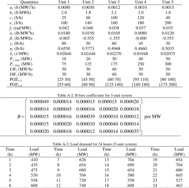
cost and emission functions are used. The fuel cost coefficients including valve-point effects, emission coefficients, generation limits, ramp rate limits, prohibited operating zones, B-loss coefficients, and load demand in each interval are given in Appendix, which is taken from [22]. The demand of the system has been divided into 24 intervals. The transmission losses are calculated using B-loss coefficients formula. The parameters of algorithm used for simulation are: max generation = 100; population size = 20; A = 0.9; r = 0.1; fmin = 0 and fmax = 2.

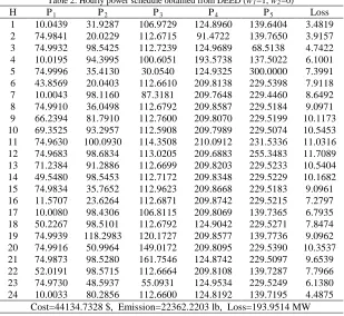
The best solutions of the dynamic economic dispatch (DED), dynamic economic emission dispatch (DEED) and pure dynamic emission dispatch (PDED) are given in Tables 2, 3, and 4, respectively.

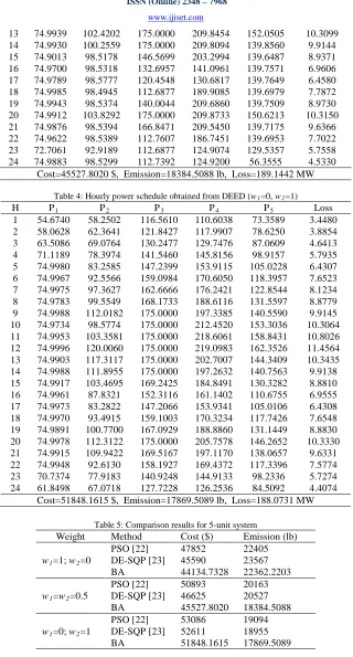
Table 2 shows hourly generation schedule, cost and emission obtained from DED problem. Table 4 shows hourly generation schedule, cost, and emission obtained from PDED problem. It is seen from Tables 2 and 4 that the cost is 44134.7328 $ under DED but it increases to 51848.1615 $ under PDED and emission obtained from DED is 22362.2203 lb but decreases to 17869.5089 lb under PDED. Table 3 shows hourly generation schedule, cost, and emission obtained from DEED problem. It can be seen that the cost is 45527.8020 $ which is more than 44134.7328 $ and less than 51848.1615 $, and emission is 18384.5088 lb which is less 22362.2203 lb and more than 17869.5089 lb.

Table 2: Hourly power schedule obtained from DEED (w1=1, w2=0)

H P1 P2 P3 P4 P5 Loss

1 10.0439 31.9287 106.9729 124.8960 139.6404 3.4819 2 74.9841 20.0229 112.6715 91.4722 139.7650 3.9157 3 74.9932 98.5425 112.7239 124.9689 68.5138 4.7422 4 10.0195 94.3995 100.6051 193.5738 137.5022 6.1001 5 74.9996 35.4130 30.0540 124.9325 300.0000 7.3991 6 43.8569 20.0403 112.6610 209.8138 229.5398 7.9118 7 10.0043 98.1160 87.3181 209.7648 229.4460 8.6492 8 74.9910 36.0498 112.6792 209.8587 229.5184 9.0971 9 66.2394 81.7910 112.7600 209.8070 229.5199 10.1173 10 69.3525 93.2957 112.5908 209.7989 229.5074 10.5453 11 74.9630 100.0930 114.3508 210.0912 231.5336 11.0316 12 74.9683 98.6834 113.0205 209.6883 255.3483 11.7089 13 71.2384 91.2886 112.6699 209.8203 229.5233 10.5404 14 49.5480 98.5453 112.7172 209.8348 229.5229 10.1682 15 74.9834 35.7652 112.9623 209.8668 229.5183 9.0961 16 11.5707 23.6264 112.6871 209.8742 229.5215 7.2797 17 10.0080 98.4306 106.8115 209.8069 139.7365 6.7935 18 50.2267 98.5101 112.6792 124.9042 229.5271 7.8474 19 74.9939 118.2983 120.1727 209.8577 139.7736 9.0962 20 74.9916 50.9964 149.0172 209.8095 229.5390 10.3537 21 74.9873 98.5280 161.7546 124.8742 229.5097 9.6539 22 52.0191 98.5715 112.6664 209.8108 139.7287 7.7966 23 74.9730 48.5937 55.0931 124.9534 229.5249 6.1380 24 10.0033 80.2856 112.6600 124.8192 139.7195 4.4875

Cost=44134.7328 $, Emission=22362.2203 lb, Loss=193.9514 MW

Table 3: Hourly power schedule obtained from DEED (w1=w2=0.5)

H P1 P2 P3 P4 P5 Loss

13 74.9939 102.4202 175.0000 209.8454 152.0505 10.3099 14 74.9930 100.2559 175.0000 209.8094 139.8560 9.9144 15 74.9013 98.5178 146.5699 203.2994 139.6487 8.9371 16 74.9700 98.5318 132.6957 141.0961 139.7571 6.9606 17 74.9789 98.5777 120.4548 130.6817 139.7649 6.4580 18 74.9985 98.4945 112.6877 189.9085 139.6979 7.7872 19 74.9943 98.5374 140.0044 209.6860 139.7509 8.9730 20 74.9912 103.8292 175.0000 209.8733 150.6213 10.3150 21 74.9876 98.5394 166.8471 209.5450 139.7175 9.6366 22 74.9622 98.5389 112.7607 186.7451 139.6953 7.7022 23 72.7061 92.9189 112.6877 124.9074 129.5357 5.7558 24 74.9883 98.5299 112.7392 124.9200 56.3555 4.5330

Cost=45527.8020 $, Emission=18384.5088 lb, Loss=189.1442 MW

Table 4: Hourly power schedule obtained from DEED (w1=0, w2=1)

H P1 P2 P3 P4 P5 Loss

1 54.6740 58.2502 116.5610 110.6038 73.3589 3.4480 2 58.0628 62.3641 121.8427 117.9907 78.6250 3.8854 3 63.5086 69.0764 130.2477 129.7476 87.0609 4.6413 4 71.1189 78.3974 141.5460 145.8156 98.9157 5.7935 5 74.9980 83.2585 147.2399 153.9115 105.0228 6.4307 6 74.9967 92.5566 159.0984 170.6050 118.3957 7.6523 7 74.9975 97.3627 162.6666 176.2421 122.8544 8.1234 8 74.9783 99.5549 168.1733 188.6116 131.5597 8.8779 9 74.9988 112.0182 175.0000 197.3385 140.5590 9.9145 10 74.9734 98.5774 175.0000 212.4520 153.3036 10.3064 11 74.9953 103.3581 175.0000 218.6061 158.8431 10.8026 12 74.9996 120.0060 175.0000 219.0983 162.3526 11.4564 13 74.9903 117.3117 175.0000 202.7007 144.3409 10.3435 14 74.9988 111.8955 175.0000 197.2632 140.7563 9.9138 15 74.9917 103.4695 169.2425 184.8491 130.3282 8.8810 16 74.9961 87.8321 152.3116 161.1402 110.6755 6.9555 17 74.9973 83.2822 147.2066 153.9341 105.0106 6.4308 18 74.9970 93.4915 159.1003 170.3234 117.7426 7.6548 19 74.9891 100.7700 167.0929 188.8860 131.1449 8.8830 20 74.9978 112.3122 175.0000 205.7578 146.2652 10.3330 21 74.9915 109.9422 169.5167 197.1170 138.0657 9.6331 22 74.9948 92.6130 158.1927 169.4372 117.3396 7.5774 23 70.7374 77.9183 140.9248 144.9133 98.2336 5.7274 24 61.8498 67.0718 127.7228 126.2536 84.5092 4.4074

Cost=51848.1615 $, Emission=17869.5089 lb, Loss=188.0731 MW

Table 5:Comparison results for 5-unit system

Weight Method Cost ($) Emission (lb)

w1=1; w2=0

PSO [22] 47852 22405 DE-SQP [23] 45590 23567 BA 44134.7328 22362.2203

w1=w2=0.5

PSO [22] 50893 20163 DE-SQP [23] 46625 20527 BA 45527.8020 18384.5088

w1=0; w2=1

PSO [22] 53086 19094 DE-SQP [23] 52611 18955 BA 51848.1615 17869.5089

Table 5 shows that the efficiency of the proposed method compares with other method for DEED problem at different weighting factors. It can be seen that both fuel

www.ijiset.com

5. Conclusions

In this paper, Bat Algorithm (BA) has been successfully applied for solving the DEED problem considering ramp rate limits, valve-point effects, prohibited operating zones, and transmission loss. The effectiveness of this algorithm is demonstrated for a 5-unit generation system. The obtained results from the test systems have indicated that the proposed technique has a much better performance in terms of the lowest fuel cost and emissions than other optimization methods reported in the literature. From the results obtained it can be concluded that proposed BA based approach is a competitive technique for solving complex non-smooth optimization problems in power system operation.

References

[1] X. S. Han, H. B. Gooi, D. S. Kirschen, “Dynamic economic dispatch: feasible and optimal solutions”, IEEE Transactions on Power Systems, vol.16, no.1, pp.22-28, 2001.

[2] X. Xia, A. M. Elaiw, “Optimal dynamic economic dispatch of generation: a review”, Electric Power Systems Research, vol. 80, no. 8, pp. 975- 986, 2010. [3] T. A. A. Victoire and A. E. Jeyakumar,

“Deterministically guided PSO for dynamic dispatch considering valve-point-effects,” Electric Power Systems Research, vol. 73, no. 3, pp. 313-322, 2005.

[4] X. Yuan, A. Su, Y. Yuan, H. Nie and L. Wang, “An improved PSO for dynamic load dispatch of generators with valve-point effects”, Energy, vol. 34, pp. 67-74, 2009.

[5] Z. L. Gaing, “Constrained dynamic economic dispatch solution using particle swarm optimization,” IEEE Power Engineering Society General Meeting, vol. 1, pp. 153-158, 2004.

[6] M. Basu, “Artificial immune system for dynamic economic dispatch,” International Journal of Electrical Power & Energy Systems, vol. 33, no. 1, pp. 131-136, 2011.

[7] F. Benhamida et al., “A solution to dynamic economic dispatch with prohibited zones using a Hopfield neural network,” 7th

International Conference on Electrical and Electronic Engineering, pp. 423-427, Bursa, Turkey, 1-4 December 2011.

[8] M. A. Abido, “Environmental/economic power dispatch using multi-objective evolutionary algorithms”, IEEE Transactions on Power Systems, vol. 18, no. 4, pp. 1529-1537, 2003.

[9] M. Basu, “Evolutionary programming-based goal-attainment method for economic emission load dispatch with non-smooth fuel cost and emission level functions”, Journal of The Institution of Engineers (India), vol. 86, pp. 95-99, 2005.

[10] U. Guvence, “Combined economic emission dispatch solution using genetic algorithm based on similarity crossover”, Sci. Res. Essay, vol. 5, no. 17, pp. 2451-2456, 2010.

[11] Y. Sonmez, “Multi-objective environmental/ economic dispatch solution with penalty factor using artificial bee colony algorithm”, Sci. Res. Essay, vol. 6, no. 13, pp. 2824-2831, 2011.

[12] J. B. Park, K. S. Lee, J. R. Shin and K. Y. Lee, “A particle swarm optimization for economic dispatch with nonsmooth cost functions,” IEEE Transactions on Power Systems, vol. 20, no. 1, pp. 34-42, 2005.

[13] M. A. Abido, “A novel multiobjective evolutionary algorithm for environmental/ economic power dispatch”, Electric Power Systems Research, vol. 65, pp. 71-81, 2003.

[14] H. T. Yang, P. C. Yang and C. L. Huang, “Evolutionary programming based economic dispatch for units with non-smooth fuel cost functions,” IEEE Transactions on Power Systems, vol. 11, no. 1, pp. 112-118, 1996. [15] Z. L. Gaing, “Particle swarm optimization to solving the

economic dispatch considering the generator constraints,” IEEE Transactions on Power Systems, vol. 18, no. 3, pp. 1187-1195, 2003.

[16] S. Duman, U. Guvenc and N. Yorukeren, “Gravitational search algorithm for economic dispatch with valve-point effects,” International Review of Electrical Engineering, vol. 5, no. 6, pp. 2890-2895, 2010.

[17] R. Balamurugan and S. Subramanian, “An improved differential evolution based dynamic economic dispatch with nonsmooth fuel cost function”, Journal of Electrical Systems, vol. 3, no. 3, pp. 151-61, 2007.

[18] B. Mohammadi–ivatloo, A. Rabiee and M. Mehdi Ehsan, “Time varying acceleration coefficients IPSO for solving dynamic economic dispatch with non-smooth cost function”, Energy Conversion and Management, vol. 56, pp. 175-183, 2012.

[19] B. Mohammadi–ivatloo, A. Rabiee, A. Soroudi and M. Mehdi Ehsan, “Imperialist competitive algorithm for solving non-convex dynamic economic power dispatch”, Energy, vol. 44, pp. 228-240, 2012.

[20] Rajkumari Batham, Kalpana Jain, and Manjaree Pandit, “Improved particle swarm optimization approach for nonconvex static and dynamic economic power dispatch”, International Journal of Engineering, Science and Technology, vol. 3, no. 4, pp. 130-146, 2011. [21] X.-S. Yang, “A new metaheuristic bat-inspired

algorithm, in nature inspired cooperative strategies for optimization”, (NICSO 2010) (Eds. J. R. Gonzalez et al.), Studies in Computational Intelligence, Springer Berlin, Springer, 284, pp. 65-74, 2010.

[22] M. Basu, “Particle swarm optimization based goal-attainment method for dynamic economic emission dispatch,” Electric Power Components and Systems, vol. 34, pp. 1015-1025, 2006.

Scientific & Engineering Research, vol. 6, no. 10, pp. 1136-1141, 2015.

Appendix

Table A-1: Data for the 5-unit system

Quantities Unit 1 Unit 2 Unit 3 Unit 4 Unit 5 ai ($/(MW)2h) 0.0080 0.0030 0.0012 0.0010 0.0015

bi ($/MWh) 2.0 1.8 2.1 2.0 1.8

ci ($/h) 25 60 100 120 40

ei ($/h) 100 140 160 180 200

fi(rad/MW) 0.042 0.040 0.038 0.037 0.035

αi (lb/MW2h) 0.0180 0.0150 0.0105 0.0080 0.0120

βi (lb/MWh) -0.805 -0.555 -1.355 -0.600 -0.555

γi (lb/h) 80 50 60 45 30

ηi (lb/h) 0.6550 0.5773 0.4968 0.4860 0.5035

δi (1/MW) 0.02846 0.02446 0.02270 0.01948 0.02075

Pi, min (MW) 10 20 30 40 50

Pi, max (MW) 75 125 175 250 300

URi (MW/h) 30 30 40 50 50

DRi (MW/h) 30 30 40 50 50

POZs-1 [25 30] [45 50] [60 70] [95 110] [80 100]

POZs-2 [55 60] [80 90] [125 140] [160 180] [175 200]

Table A-2: B-loss coefficients for 5-unit system

MW per

000035 . 0 000014 . 0 000012 . 0 000018 0 000020 . 0

000014 . 0 000040 . 0 000010 . 0 000020 0 000015 . 0

000012 . 0 000010 . 0 000039 . 0 000016 0 000015 . 0

000018 . 0 000020 . 0 000016 . 0 000045 0 000014 . 0

000020 . 0 000015 . 0 000015 . 0 000014 0 000049 . 0

     

 

     

 

=

. . . . .

B

Table A-3: Load demand for 24 hours (5-unit system) Time

(h)

Load (MW)

Time (h)

Load (MW)

Time (h)

Load (MW)

Time (h)

Load (MW)

1 410 7 626 13 704 19 654

2 435 8 654 14 690 20 704

3 475 9 690 15 654 21 680

4 530 10 704 16 580 22 605

5 558 11 720 17 558 23 527

6 608 12 740 18 608 24 463