Body Shape and Complex Permittivity Determination Using
the Method of Auxiliary Sources
Vasil Tabatadze1, 2, *, Kamil Kara¸cuha1, and Ertuˇgrul Kara¸cuha1
Abstract—In this article, the body shape and complex permittivity determination employing inverse electromagnetic scattering problem solution for two-dimensional cases is considered. The method of auxiliary sources (MAS) is used as a mathematical apparatus. Several body shape cases are considered, and the efficiency of the approach is shown. The program package is created based on this method, and the numerical experiment results are presented.
1. INTRODUCTION
For fifty years, inverse scattering problem has kept its importance and popularity because its ultimate purpose to determine physical and geometric properties of an inaccessible object without invasive methods which is always studied and appeals researchers through this branch of science. In such problems, the body can have mainly two essential properties.They are geometric properties which are the position and shape of the object, and physical properties which can be expressed with constitutive parameters. To find these main features, generally, the information contained in the scattered field distribution by this object is studied, when the object is illuminated by the wave source. Here, we only deal with electromagnetic waves in order to find main properties of the object. In this study, the body is located at an unbounded and homogeneous free space. Such a case is crucial for military, space, telecommunication, satellite applications.
There exist several methods for this problem solution. By the authors of this article, there are several published articles in this direction [1–4]. In studies [1, 2], the authors only focused on the body shape and location determination. Under some specific conditions and estimations, there exist many highly accurate analytical and numerical methods for solving the inverse scattering problem. In article [5], the author used the double Fourier transform for the inverse problem solution. Furthermore, there are some other analytical and numerical works related to this topic [6–14]. There are also other authors who used the Method of Auxiliary Sources to solve direct scattering problem [15–17].
A underlying assumption has been commonly made in many studies related to cylindrical bodies with infinite length in a specific direction. Studies starting with this assumption are done very frequently because of two reasons. First, the investigation is slightly simpler than other problems, and secondly, such objects have a similar geometry to real-world objects. In this article, we also deal with such an object. Here, a two-dimensional case is considered when the object is infinite in the third dimension.
The novelty of our article is that it solves this problem using MAS and expands the possibility of this method not only for body shape determination but also for complex permittivity determination. The body of interest is illuminated from many different locations, and the scattered field is measured at some circular curve contour. During the real experiment, it is needed to realize many measurements from different positions at several frequencies in order to get higher accuracy of the solution. In the
Received 9 October 2019, Accepted 23 November 2019, Scheduled 13 December 2019 * Corresponding author: Vasil Tabatadze ([email protected]).
1 Informatics Institute of Istanbul Technical University, Maslak, Istanbul 34469, Turkey. 2 Tbilisi State University, 1 Chavchavadze
scope of this article, our investigation is based on the simulation. Note that in order to get the scattered field, the direct problem is also solved.
In Section 2, the theoretical background for the direct and inverse problem and the numerical approach is mainly presented. In the following section, the results are given. In Section 4, the comparison of the results obtained with our method and the other method is given. After that, the conclusion is drawn.
2. THEORETICAL BACKGROUND
In the theoretical part, the problem statement, field extremum on the boundary of two media, direct problem solution using the MAS, inverse problem solution again using the MAS and determination of the object complex permittivity are explained in detail.
2.1. Problem Statement
The problem statement, mathematical background, and application point of view are drawn in the section. Suppose that there is an object which in general has unknown complex Permittivity. In Figure 1, the problem statement is given. This non-magnetic object is radiated by a point source located near the object (Figure 1). The object reradiates scattered field. The scattered field Esc satisfies the next well-known relation given in Eq. (1). Keep in mind that, here, the two-dimensional problem is considered, and the electric field has only z-component.
Esc(rout) =
CH (1)
0 (k|rout−r|)ν(r) [Einc(r) +Eout(r)]dxdy (1)
Here,Esc(rout) is the scattered field at some point outside the object of interest; ν is called the object function given in Eq. (2); andC in the integral is the contour of the object.
ν(r) = 1 0
(r) +iσ(r) ω
−1 (2)
Here,(r) is the complex permittivity of the object which is, in general, the function of the coordinate, conductivity σ(r), angular frequencyω, wavenumber k, and incident electric fieldEinc(r). If the Born approximation is used, inside the integral, there will be only the incident electric field as in Eq. (3).
Esc(rout) =
CH (1)
0 (k|rout−r|)ν(r)Einc(r)dxdy (3)
Note that the approximation works for small values of the object function and wave number. The term which is neglected has asymptotical behavior O(k4||ν||2). Initially, the object function is unknown. If this function is determined, the complex permittivity given in Eq. (4) can be found.
(r) +iσ(r)
ω =0(ν(r) + 1) (4)
Consider the case when there is a smooth object with constant permittivity (r) = c. Here, c is a constant. In this case, the object function can be taken outside the integral.
Esc(rout) =ν
CH (1)
0 (k|rout−r|)Einc(r)dxdy (5)
In order to find ν, it is needed to take the integral (the incident field distribution is known) and to measure the scattered field in a point. Therefore, this problem is very easily solved. However, the difficulty arises when the contour of integration is not known. In other words, the shape of the object and its exact location are not known. This means that one cannot measure the object, directly. For example, it is the case when a satellite orbits around some asteroids and tries to determine the electric properties of the asteroids. Also, there can be the case when the object is not reachable for human, and the only way is to send a drone to inspect the object by using electromagnetic waves. There can be other situations on earth when one cannot reach the object of interest to measure it, but one can go around the object, illuminate with a source, and measure the scattered field. Therefore, the first goal is to determine the shape of the object and its location in space. This problem could be generalized when the object of interest is embedded in some media. In that case, the hidden object is not seen directly, and the only way is to investigate its properties using electromagnetic radiation. However, this article only considers the case when the object is located in free space.
2.2. Determination of the Field Extremum on the Boundary of Two Media
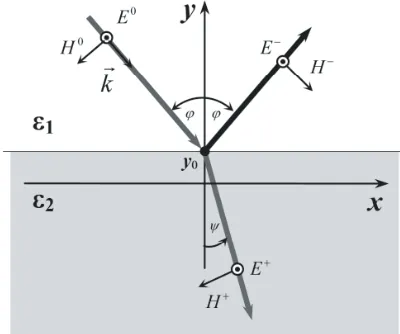
Before going to the main problem, it is better to highlight the fundamental property of the electromagnetic fields at the border of two dielectrics. For simplicity, it is an acceptable idea to consider the case when we have the infinite planar boundary of two media with permittivity’s ε1 and ε2 given in Figure 2. Note that the incidence wave is a plane wave and time dependency eiωt.
Figure 2. The diffraction by the infinite planar boundary of the two media.
Respectively, the incident, reflected and transmitted field can be given as in Eq. (6).
Einc(r) ˆaz =E0(r) =E0e(−ik(xsinφ−(y−y0) cosφ))ˆaz E−ˆaz =E0ρ⊥e(−ik(xsinφ+(y−y0) cosφ))aˆz E+ˆaz =E0τ⊥e(−ik(xsinφ+(y−y0) cosψ))aˆz
(6)
Here,ρ⊥ and τ⊥ are the reflection and transmission coefficients, respectively, and ˆaz is the unit vector directed through the z-axis. Let us introduce the next integral given in Eq. (7) and solve it.
P(y) = k2
k1
E0+E−2dk=E02(k2−k1)
1 +ρ2⊥+ 2ρ⊥sinα α cosβ
where, β= (y−y0)(k2+k1) cosφand α= (y−y0)(k2−k1) cosφ.
Now, it is time to find the extremums of Eq. (7). It can be easily shown that
min [P(y)] = E02(k2−k1) (1 +ρ⊥)2=P(y0) ifρ⊥<0 and2 > 1
max [P(y)] = E02(k2−k1) (1 +ρ⊥)2=P(y0) ifρ⊥>0 and2 < 1
Here, min and max stand for the minimum and maximum values of the function, respectively.
In both cases, we have the extremum at the boundary of two dielectric media, and this result can be generalized for other shapes of the boundary. Therefore, it is needed to know the scattered field distribution along the boundary of two media, and then, the integration of the electric field in frequency range from k1 to k2 is required as given in Eq. (8). Therefore, we have to find the analog of the P(y) function which will be, in our case, the function of coordinate variablesP(x, y).
P(x, y) = k2
k1
E0(x, y) +E−(x, y)2dk (8)
During the numerical experiment, the integral is substituted by the sum as in Eq. (9).
P(x, y) = k2
k=k1
E0(x, y) +E−(x, y)2Δk (9)
We should choose the range of x ∈ [x1, x2] and y ∈ [y1, y2] so that it should occupy the object of interest. The first aim is to find the distribution of P(x, y) function. The next step is to find the minimum (or maximum) area inP(x, y) which corresponds to the boundary of two media. This gives an ability to reconstruct the shape of the scattering object. However, in order to determineP(x, y) function, it is needed to know the scattered electric field value in the rangesx∈[x1, x2] andy ∈[y1, y2]. Keep in mind that the incident field is initially given and known. During the real experiment, it is necessary to conduct measurements of the scattered field. We have to take into account the fact thatP(x, y) requires the scattered electric field distribution for different frequencies in the range of wavenumberk∈[k1, k2]. In our case, the real experiments is substituted by the direct problem solution of the diffraction problem. For this, MAS is used which is discussed in the following part [4].
2.3. Direct Problem Solution Using the MAS
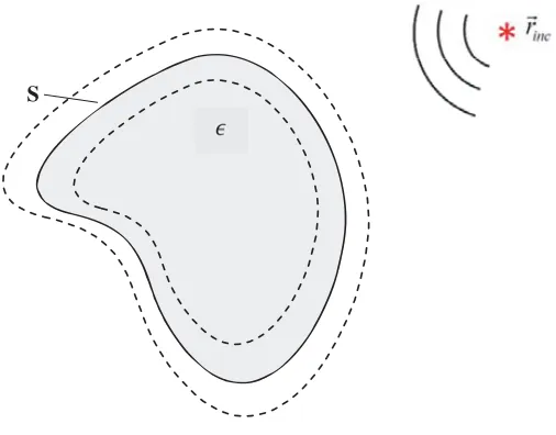
The MAS gives an ability to solve the diffraction problem of electromagnetic waves of the cylinder source by the 2D complex shape object (with the contour S) with complex permittivity (Figure 3). The permittivity of the area outside the object contour corresponds to the vacuum.
The electric field of the cylinder source can be expressed as Einc(r) = H0(1)(k|r−rinc|). H (1) 0 is the Hankel’s function of the first kind and zero-order, andrinc is the location of the line source. The observation point is given as r = (x, y). The electric field has only z-component which is normal to the object contour. Outside and inside theS contour, there are constructed inner and outer auxiliary contours. Inner contour describes the electric field distribution outside the scatterer. Outer contour describes the field inside the scatterer. Mathematically, the electric field outside the scatterer is the sum of the field by the incident source and the field radiated by the inner auxiliary surface as given in Eq. (10).
Eout(x, y) = N
n=1
XninH01
kout(x−xin)2+ (y−yin)2 +Einc(x, y) (10)
Here,Xnin are unknown complex amplitudes of the auxiliary sources distributed on the inner auxiliary contour. Then, the electric field inside the scatterer is expressed as in Eq. (11)
Ein(x, y) = N
n=1
XnoutH01
kin
S
Figure 3. The geometry of the scatterer object.
Here,Xnout are unknown complex amplitudes of the auxiliary sources distributed on the outer auxiliary contour. In order to find these unknown coefficients, the boundary condition satisfaction on the scatterer’s surface is required. For the dielectric media, boundary condition means that the tangential components of the electric and magnetic fields should be continuous along the scatterer surface.
Ein(xm, y) =Eout(xm, y), Hin(xm, ym) =Hout(xm, ym). (xm, ym) are the points on theS surface.
Magnetic field strength (H) is found by Maxwell’s equation given as follows.
rotE =−iωμ H
After requiring these boundary conditions on the scatterer’s surface, the linear algebraic equation system with respect to the unknowns Xnin and Xnout is achieved. After solving this linear algebraic equation system, unknown coefficients are determined. Then, the field distributions due to the scatterer are found inside and outside. The values of the scattered field will be used for the next step when the inverse problem is solved.
2.4. Inverse Problem Solution Using the MAS
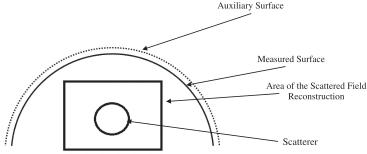
We determine the scattered field with the method described in Section 2.3 on a semicircle (Figure 4) which contains the scatterer object.
During the real experiment, instead of solving the diffraction problem by the scatterer, we should measure the field values on this semicircle (Figure 4) which we call measured surface. The MAS gives an ability to reconstruct the scattered field in the rectangular area shown in Figure 4.
Let’s formulate the MAS for the inverse problem solution. We construct an auxiliary semicircle contour near the measured surface. The reconstructed scattered field Erec(x, y) can be expressed as Eq. (12).
Erec(x, y) = N
n=1
XnH0(2)
(x−xn)2+ (y−yn)2 (12)
Here, Xn are unknown coefficients of the auxiliary sources to be determined. H0(2) is the Hankel’s function of the second kind and zero-order, which describes the absorbing wave. In order to find Xn coefficients, the boundary condition satisfaction on the measured surface is required. In Eq. (12), xn and yn are the auxiliary source locations, and x and y are any points in the reconstructed area. The reconstructed field on this surface must be the same as the measured field as given in Eq. (13).
Scatterer
Auxiliary Surface
Measured Surface
Area of the Scattered Field Reconstruction
Figure 4. Inverse problem solution.
Here,N is the number of collocation points where the boundary condition satisfaction is required. As a result, we get the linear algebraic equation system after the solution of which we find the unknown coefficients. After that, it is possible to reconstruct the scattered field in the rectangular area shown in Figure 4. Then, it is possible to find functionP(x, y) with Eq. (9).
The next step is to find its minimum value ofP(x, y) and then, to find the body shape and location. However, if we radiate the object from one side, it can reconstruct only a part of the object surface, because the auxiliary surface is not closed. Therefore, in order to find the whole surface of the scatterer, we have to conduct many measurements. We should change the location of the incident field source and at the same time, should rotate the measured surface. Finally, we have to add the obtainedP(x, y) function distribution for different source locations, and we will see the extremum of P(x, y) on this distribution. After that, it is necessary to extract the body contour from this minimum area. Because we have the numerical data, it is easy to determine in which pointsP(x, y) is minimum. As a result, we get the object contour with some thickness. Thickness depends on the choice of the wavelength range. Finally, we should filter the data to extract the object contour.
2.5. Determination of the Object Complex Permittivity
As mentioned above, the Born approximation given in Eq. (5) is used in order to evaluate complex permittivity. This time, it needs one more extra measurement to get the scattered field in the point outside the scatterer. In our case, we find this value by the direct problem solution described in Section 2.3. The wavenumber is chosen so that it is compatible with the Born approximation. In this study, the wavenumber equalsk= 0.25. Because in the previous stage, we have determined the contour shape, we can take integral given in the right part of Eq. (5). Here, the incident wave is initially given, and the Hankel argument contains all the known variables. Therefore, we divide the scattered field given in the left part by the integral value, and we get object function ν. Finally, from Eq. (4), the value of the complex permittivity can be found.
3. RESULTS OF THE NUMERICAL SIMULATION
In this section, results of the numerical simulations are presented for the stages of reconstruction procedure and also for different shapes.
Figure 5. Step by step reconstruction of the circle surface (P(x, y) distribution function for different incident angles).
(a) (b)
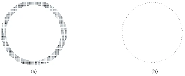
Figure 6. The reconstructed contour of the scatterer: (a) In first approximation, (b) the final contour.
the final reconstructed surface. The number of sensors on the measured surface that we take for all cases is 100. In total, 21 different angle measurements are needed to get solution less than 3%. The error of solution does not change much by changing the geometry. Therefore, 21 different angles are optimal for all cases considered below. For example, 10 different angles give accuracy 5%, and 5 different angles give 14% error.
As seen, we get a circle shape spot object as a result if we extract corresponding points of space, and we get the next image in Figure 6(a). We should extract the contour with possibly minimal width from this aggregate of points. We do it using a computer program. We filter these points and get the contour as in Figure 6(b).
As the contour is found, we can find the object functionv from Eq. (5) and determine the complex values for the permittivity. The reconstructed value of the permittivity is = 3.94. The accuracy of the solution is 98.5%. The error that we get is the result of reconstructed contour shape deviation from the real contour.
We also consider the case of an ellipse (with parameters 1 m×0.5 m), and the corresponding results are shown in Figure 7. In Figure 7, (a) corresponds to the reconstructed function P(x, y); (b) is the contour reconstruction in the first approximation; and (c) is the final reconstructed contour.
In the case of an ellipse, the reconstructed value is = 3.92. The error of the permittivity value determination is a little higher and is about 2%. This is also due to the deviation of the reconstructed contour from the real one.
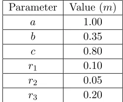
An object with a more complicated shape is also considered which is given on Figure 8. The geometry of the object is composed by line segments and circle sectors. Dimensions of the object are listed in Table 1.
(a) (b) (c)
Figure 7. The reconstructed contour of the scatterer: (a)P(x, y) function distribution, (b) the contour in the first approximation, (c) the final contour.
Figure 8. The geometry of the object with complicated shape.
Table 1. Parameters and their values for Figure 7.
Parameter Value (m)
a 1.00
b 0.35
c 0.80
r1 0.10
r2 0.05
r3 0.20
(a) (b) (c)
Figure 9. The reconstructed contour of the scatterer: (a)P(x, y) function distribution, (b) the contour in the first approximation, (c) the final contour.
The reconstructed value of the permittivity is 3.86. The error of solution is 3.5%. The error is slightly higher than the previous cases. Again the reason is the contour reconstruction error. However, in all three cases, the error is less than 4%.
We also consider the case when the conductivity is not zero. Forσ = 3000000 Ω−1, the reconstructed value of the permittivity () given in Eq. (4) is 3.86, and the reconstructed value of the conductivity is σ = 2991721 Ω−1. The error of the permittivity is again 3.5%, and error of conductivity is 0.3%. Note that we do not consider higher values of permittivity. After >5, the error becomes more than 5%. In order to increase accuracy, it is needed to consider higher frequencies, and more measurements need to be carried out.
4. COMPARISON WITH OTHER METHOD
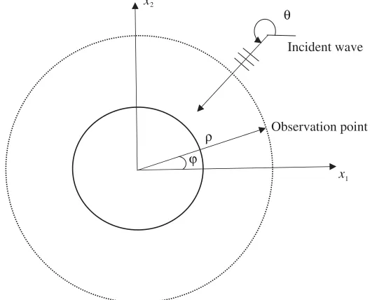
In this section, we present the comparison of the results obtained by our method and the analytical method described in the work [18]. The object of interest is a circle with radius 1 and permittivity = 1.1. The geometry for the inverse problem analytical solution is given in Figure 10. In order to
Observation point Incident wave
x x
1 2
θ
ϕ ρ
solve the inverse problem and find the permittivity distribution with analytical method [18], the object of interest is irradiated by the plane wave with the angle of incidence θ. After that, the scattered field is measured on the circular surface (dotted circle Figure 10) for differentϕ values. The next step is to find the Fourier transform of the object function which can be expressed as:
ˆ
v[k(cosϕ−cosθ), k(sinϕ−sinθ)] =
√
8kπ k2 e−i
π
4|x|e−ik|x|us(x)
wherekis the wave number;x= (x1, x2) is the point in which the scattered field is measured (observation point); us(x) is the scattered field measured in point x.
After that, we calculate the object function in pointx0= (x10, x20) with the next formula:
v(x10, x20) = k 2
(2π)2 π
−π dθ
θ
θ−π ˆ
v[k(cosϕ−cosθ), k(sinϕ−sinθ)]eik((cosϕ−cosθ)x10+(sinϕ−sinθ)x20) dϕ
We calculate the object function with this formula along thex1 axis in the range (−1.5, 1.5) and after that evaluate the permittivity value using Eq. (4).
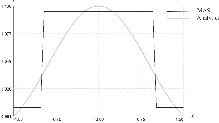
Figure 11 shows the comparison between the results obtained with the analytical method and that with the MAS. The value of wave number for the analytical method case isk= 1.25 m−1, and the radius of the circle on which the scattered field is evaluated isρ= 50 m.
MAS Analytical
x1
Figure 11. Reconstruction of the permittivity distribution obtained by two different methods: with MAS and with the analytical method.
As shown in the figure, our method gives a stepwise solution with correct values of the permittivity, and the analytical method gives the results with smoothly changing values of permittivity with some deviation from real value. This comparison emphasizes the efficiency of our method.
5. CONCLUSION
REFERENCES
1. Tabatadze, V., M. Prishvin, G. Saparishvili, D. Kakulia, and R. Zaridze, “Soil’s characteristics study and buried objects visualization using remote sensing,” Proceedings of XIIth International Seminar/Workshop on Direct and Inverse Problems of Electromagnetic and Acoustic Wave Theory
(DIPED-2007), 134–138, Tbilisi, Georgia, Sep. 17–20, 2007.
2. Tabatadze, V., D. Kakulia, G. Saparishvili, R. Zaridze, and N. Uzunoglou, “Development of an new efficient numerical approach for object recognition,” Journal of Applied Electromagnetism, Vol. 12, 35–36, Nov. 18, 2008.
3. Tabatadze, V., D. Kakulia, G. Saparishvili, R. Zaridze, and N. Uzunoglou, “Development of a new efficient numerical approach for buried object recognition,”Sensing and Imaging: An International
Journal, Vol. 1, No. 1, 35–56, 2011.
4. Zaridze, R., G. Bit-Babik, K. Tavzarashvili, N. K. Uzunoglu, and D. Economou, “The method of auxiliary sources (MAS) — Solution of propagation, diffraction and inverse problems using MAS,”
Appl. Comput. Electromagn., 33–45, Springer, 2000.
5. Karacuha, E., “Determination of the orientation of cylindrical bodies buried in a slab from the scattering date,” MMET’96, VIth Int. Conf. Math. Methods Electromagn. Theory Proc., 444–448, IEEE, 1996.
6. Peterson, E., “The σ-orientation,” Form. Geom. Bordism Oper., 219–282, 2018, doi: 10.1017/9781108552165.008.
7. ˙Idemen, M. and ˙I. Akduman, “On inverse scattering problems related to cylindrical bodies with unknown orientations,”Wave Motion, Vol. 17, 33–48, 1993.
8. Idemen, M. and I. Akduman, “Some geometrical inverse problems connected with two-dimensional static fields,”SIAM J. Appl. Math., Vol. 48, 703–718, 1988.
9. Anastassiu, H. T., D. I. Kaklamani, D. P. Economou, and O. Breinbjerg, “Electromagnetic scattering analysis of coated conductors with edges using the method of auxiliary sources (MAS) in conjunction with the standard impedance boundary condition (SIBC),”IEEE Trans. Antennas
Propag., Vol. 50, 59–66, 2002.
10. Abubakar, A., P. M. van den Berg, and S. Y. Semenov, “Two- and three-dimensional algorithms for microwave imaging and inverse scattering,” Journal of Electromagnetic Waves and Applications, Vol. 17, No. 2, 209–231, 2003.
11. Colton, D. and R. Kress, Integral Equation Methods in Scattering Theory, Classics in Applied
Mathematics, SIAM, Philadelphia, PA, 2013.
12. Colton, D. and R. Kress, Inverse Acoustic and Electromagnetic Scattering Theory, 3rd edition, Vol. 93, Applied Mathematical Sciences, Springer-Verlag, New York, NY, 2013.
13. Meng, Q., K. Xu, F. Shen, et al., “Microwave imaging under oblique illumination,”Sensors, Vol. 16, No. 7, 1046, 2016.
14. Gintides, D. and L. Mindrinos, “The direct scattering problem of obliquely incident electromagnetic waves by a penetrable homogeneous cylinder,”J. Integral Equations Appl., Vol. 28, No. 1, 91–122, 2016.
15. Leviatan, Y., “Analytic continuation considerations when using generalized formulations for scattering problems,”IEEE Trans. Antennas Propag., Vol. 38, No. 8, 1259–1263, Aug. 1990. 16. Barnett, A. H. and T. Betcke, “Stability and convergence of the method of fundamental solutions
for Helmholtz problems on analytic domains,”J. Comput. Phys., Vol. 227, 7003–7026, Jul. 2008. 17. Tsitsas, N. L., G. P. Zouros, G. Fikioris, and Y. Leviatan, “On methods employing auxiliary sources
for 2-D electromagnetic scattering by non-circular shapes,”IEEE Trans. Antennas Propag., Vol. 66, No. 10, 5443–5452, 2018.