ABSTRACT
MELTON, CODY ALLEN. Towards Heavy Element Materials with Electronic Structure Quantum Monte Carlo Methods. (Under the direction of Dr. Lubos Mitas.)
The study of the electronic structure of atoms, molecules, clusters, and solids is inti-mately tied to our ability to develop new technologies and applications. The majority of our understanding of materials comes directly from mean-field methods, where the explicit interactions between electrons are treated in some averaged sense. However, it is clear that for strongly correlated materials, where electron-electron interactions dominate, mean-field methods fail and more accurate and explicitly correlated methods are necessary. One of the most successful approaches is Quantum Monte Carlo, in particular the fixed-node Diffusion Monte Carlo method. This method has been shown to be reliable in accurately capturing electronic correlations, and has been successfully applied to systems ranging
from complicated biomolecules to the various 3dtransition metal oxides. As computers get
larger and more powerful, such as the exascale machines coming online in the near future, Diffusion Monte Carlo is uniquely suited to tackle more difficult and complicated systems. Despite its successes, Diffusion Monte Carlo has been mostly applied to systems
contain-ing elements up to the 3d transition metals. While there are some exceptions, applications
3dtransition metals. The ideas and constructions developed in this work can be generalized for future developments of pseudopotentials for heavier elements, where spin-orbit effects will need to be introduced. Lastly, we investigate a heavy element compound using the
current standard workflows in Diffusion Monte Carlo. We study LaScO3, where both
© Copyright 2019 by Cody Allen Melton
Towards Heavy Element Materials with Electronic Structure Quantum Monte Carlo Methods
by
Cody Allen Melton
A dissertation submitted to the Graduate Faculty of North Carolina State University
in partial fulfillment of the requirements for the Degree of
Doctor of Philosophy
Physics
Raleigh, North Carolina
2019
APPROVED BY:
Dr. Jerry Whitten Dr. Alexander Kemper
Dr. Christopher Roland Dr. Lubos Mitas
DEDICATION
BIOGRAPHY
I began my path towards this thesis in Burlington, North Carolina. I lived a very normal childhood, where I spent my time outside playing sports with my friends and family. By the time I was about to enter high school, athletics had been my full focus and was what I wanted to pursue. However, an unfortunate back injury from power lifting made that dream unobtainable, and I became determined to focus on academics in order to get to college. At the time, I wanted to become a physical therapist, in order to help others like I was helped through my injury. However, throughout the course of my high school studies, I became increasingly interested in mathematics and physics. Reading books by scientists like Carl Sagan and Stephen Hawking in my spare time, I became inspired by the beauty in the Universe and decided that I wanted to become an astrophysicist and study cosmology to understand the origins of the Universe.
ACKNOWLEDGEMENTS
First and foremost, I would like to thank my advisor, Dr. Lubos Mitas. His continuous support and his ability to find interesting problems that kept me engaged was vital to my success. He created a work environment where I was treated as a colleague, which ultimately led me to work harder to try to meet his expectations.
I would like to thank all of the current and past members of my research group. In particular, I would like to thank Dr. Chandler Bennett, who has been a close colleague and friend throughout this journey. I appreciate all of the discussions we had to deepen my understanding of electronic structure, and I look forward to working together in the future.
Thanks to Dr. Luke Shulenburger and Dr. Thomas Mattsson, who provided me the opportunity to intern at Sandia National Laboratories. This experience was appreciated as it gave me the opportunity to work with new people and on new projects, unrelated to my thesis work. This deepened my understanding of electronic structure, and has given me new ideas about how to apply the knowledge and experience I have obtained from this thesis work.
TABLE OF CONTENTS
LIST OF TABLES . . . x
LIST OF FIGURES. . . xvi
Chapter 1 Introduction. . . 1
1.1 Many-body Schrödinger Equation . . . 2
1.2 The Hartree-Fock Method . . . 3
1.3 Post Hartree-Fock Methods . . . 8
1.4 Density Functional Theory . . . 10
Chapter 2 Quantum Monte Carlo . . . 16
2.1 Monte Carlo Integration . . . 16
2.2 Variational Monte Carlo . . . 20
2.2.1 The Trial Wave Function . . . 22
2.2.1.1 A(X): the Slater Part of the Wave Function . . . 24
2.2.1.2 S(X): the Jastrow Part of the Wave Function . . . 25
2.2.2 Optimization of Many-body Trial Wave Functions . . . 27
2.3 Diffusion Monte Carlo . . . 29
2.3.1 Fermion Sign Problem and the Fixed-Node Approximation . . . 34
2.3.2 Practicalities and Approximations . . . 37
2.3.2.1 Timestep Bias . . . 37
2.3.2.2 Fixed-Node Bias and Improvements . . . 38
2.3.2.3 Pseudopotentials and the Locality Approximation . . . 39
2.3.2.4 Finite-Size Effects in Periodic Boundary Conditions . . . 40
Chapter 3 Spin-Orbit Interactions in Electronic Structure Quantum Monte Carlo Methods . . . 43
3.1 Introduction . . . 44
3.2 Discussion . . . 44
3.2.1 Phase and Absolute Value . . . 44
3.2.2 Approximations . . . 44
3.2.3 Continuous Spin and its Updates . . . 45
3.2.4 Importance Sampling and Trial Function . . . 45
3.3 Results . . . 45
3.3.1 Atomic Calculations: Excitations in Pb, Bi, and W Atoms . . . 45
3.3.2 Molecular Calculations . . . 47
3.4 Conclusion . . . 47
3.5 Acknowledgements . . . 48
Chapter 4 Quantum Monte Carlo with Variable Spins . . . 49
4.1 Introduction . . . 50
4.2 Fixed-Phase Diffusion Monte Carlo (FPDMC) . . . 50
4.2.1 Fixed-phase Upper Boundary Property . . . 51
4.2.2 Fixed-phase as a Special Case of the Fixed-node . . . 51
4.2.3 Importance Sampling . . . 51
4.3 Spin Orbit Interactions . . . 52
4.3.1 AREP and SO Operators . . . 52
4.3.2 Variational Property of the Fixed-phase Method for Nonlocal, Com-plex, Hermitian Operators . . . 53
4.4 Spin Representation and Sampling . . . 54
4.4.1 Spin Representations . . . 54
4.4.2 Trial Wave Functions . . . 55
4.4.3 Evaluation of the Pseudopotential and Importance Sampling . . . 56
4.4.4 Spin Sampling . . . 57
4.5 Time Step Errors and Approximations . . . 58
4.6 Applications . . . 59
4.6.1 PbH . . . 59
4.6.2 Sn and Sn2 . . . 60
4.6.3 Electron Affinities . . . 61
4.7 Conclusions . . . 61
4.8 Acknowledgements . . . 61
4.9 References . . . 61
Chapter 5 Fixed-Node and Fixed-Phase Approximations and Their Relationship to Variable Spins in Quantum Monte Carlo . . . 63
5.1 Introduction . . . 64
5.2 Fixed-Phase Approximation . . . 65
5.3 Simple Model for Comparing Fixed-Node versus Fixed-Phase Approximations 68 5.4 Real Wave Function Recast into a Complex Form . . . 72
5.5 Conclusions . . . 75
5.6 Acknowledgements . . . 76
5.7 References . . . 76
Chapter 6 Quantum Monte Carlo with Variable Spins: Phase and Fixed-Node Approximations . . . 77
6.1 Introduction . . . 78
6.2 Fixed-Phase Spinor Diffusion Monte Carlo . . . 78
6.2.1 Fixed-phase Approximation and the Upper Bound Property . . . 78
6.2.2 Fixed-node as a Special Case of the Fixed-Phase in General . . . 79
6.2.3 Spin Representation . . . 79
6.3 Trial Wave Functions . . . 80
6.3.1 From Fixed Phase to Fixed Node . . . 80
6.3.2 Wave Functions with Full Space-spin Symmetries . . . 81
6.4 Fixed-phase Variable Spins QMC as a General Method . . . 82
6.5 Results . . . 82
6.6 Conclusions . . . 85
6.7 Acknowledgements . . . 85
6.8 References . . . 85
Chapter 7 Projector Quantum Monte Carlo with Averaged vs. Spin-Orbit Effects: Applications to Tungsten Molecular Systems . . . 87
7.1 Introduction . . . 88
7.2 Fixed-phase Diffusion Monte Carlo . . . 89
7.3 Spin-orbit Interactions and Dynamic Spins . . . 89
7.4 Results . . . 90
7.4.1 Tungsten Oxide . . . 90
7.4.2 Tunsten Dimer . . . 91
7.5 Conclusions . . . 92
7.6 Acknowledgements . . . 93
7.7 Appendix A. Supplementary data . . . 93
7.8 References . . . 93
Chapter 8 A New Generation of Effective Core Potentials from Correlated Calcu-lations . . . 95
8.1 Introduction . . . 96
8.2 Desired Properties . . . 97
8.3 Effective ECP Hamiltonian: Isospectrality on a Subspace of Valence States . 98 8.3.1 ECP form . . . 98
8.4 Optimization Methods and Constructions . . . 98
8.4.1 Objective Function with Atomic Spectral Discrepancies Only . . . 99
8.4.2 Objective Function with Spectral and Spatial Density Matrix Discrep-ancies . . . 99
8.4.3 Optimization Methods . . . 100
8.4.4 Constructed, Combined, and Iterated Schemes . . . 100
8.5 Results . . . 100
8.5.1 Boron . . . 100
8.5.1.1 Labeling . . . 101
8.5.2 Carbon . . . 102
8.5.3 Nitrogen . . . 102
8.5.4 Oxygen . . . 103
8.5.5 Sulfur . . . 103
8.7 Conclusions . . . 107
8.8 Supplementary Material . . . 108
8.9 Acknowledgements . . . 108
8.10 Conclusions . . . 109
Chapter 9 A New Generation of Effective Core Potentials from Correlated Calcu-lations: 2nd Row Elements . . . 110
9.1 Introduction . . . 111
9.2 ECP Atomic Correlation Energies . . . 112
9.3 Construction . . . 113
9.3.1 Many-body Energy Consistency . . . 113
9.3.2 Single-body Norm Conservation . . . 114
9.3.3 Weighted Combination and Core-valence Partitioning . . . 114
9.4 ECP Form . . . 115
9.5 Valence Basis Sets . . . 116
9.6 Results . . . 116
9.6.1 Sodium . . . 117
9.6.2 Magnesium . . . 118
9.6.3 Aluminum . . . 118
9.6.4 Silicon . . . 120
9.6.5 Phosphorus . . . 120
9.6.6 Sulfur . . . 121
9.6.7 Chlorine . . . 122
9.6.8 Argon . . . 122
9.6.9 Molecular Binding Parameters, Total Energies, and Core Radii . . . 122
9.7 Conclusions . . . 123
9.8 Supplementary Material . . . 124
9.9 Acknowledgements . . . 124
9.10 References . . . 124
Chapter 10 A New Generation of Effective Core Potentials from Correlated Calcu-lations: 3d Transition Metal Series. . . 126
10.1 Introduction . . . 127
10.2 Methods . . . 128
10.2.1 ECP Parameterization . . . 128
10.2.2 Objective Function and Optimization Protocols . . . 129
10.3 Results . . . 130
10.3.1 Atomic Spectra . . . 131
10.3.2 Scandium . . . 132
10.3.3 Titanium . . . 133
10.3.4 Vanadium . . . 133
10.3.6 Manganese . . . 135
10.3.7 Iron . . . 135
10.3.8 Cobalt . . . 136
10.3.9 Nickel . . . 137
10.3.10 Copper . . . 137
10.3.11 Zinc . . . 138
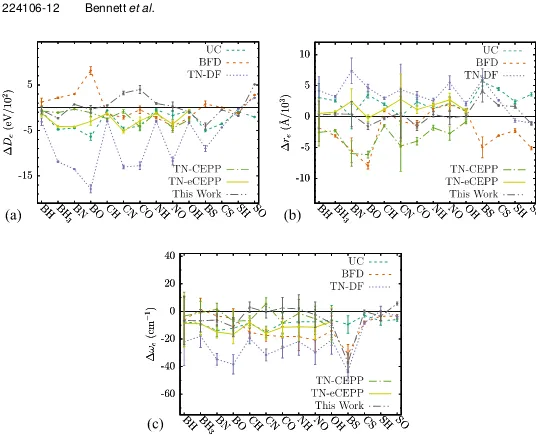
10.3.12 Average Molecular Discrepancies . . . 139
10.4 Conclusions . . . 139
Chapter 11 Many-body Electronic Structure of LaScO3by Real Space Quantum Monte Carlo . . . 141
11.1 Introduction . . . 141
11.2 Methods . . . 143
11.3 Results . . . 147
11.3.1 Bandgap of LaScO3 . . . 147
11.3.2 Cohesive Energy . . . 151
11.4 Conclusions . . . 152
LIST OF TABLES
Table 3.1 FPSODMC (DMC for short) excitation energies (eV) of the Pb atom
us-ing LC and SC relativistic PPs[17]with COSCI trial function compared
with experiment (Exp). For completeness we include also Dirac-Fock
COSCI results. The multireference CI (MRCI) and MRCI+core
po-larization corrections (CPP) calculations[17]are done with the LC
PP. . . 46
Table 3.2 FPSODMC excitation energies (eV) of the Bi atom using LC and SC
relativistic PPs[17,18], compared with experiment (Expt.). For
com-pleteness we include Dirac-Fock complete open-shell CI (COSCI) and CI (SDT) results. The second row indicates FPSODMC trial wave func-tions. . . 47
Table 3.3 DMC excitation energies (eV) of the W atom with a relativistic PP[23]
compared with CISD and experiment (Expt.). CISD is extrapolated to a complete basis set limit. . . 47
Table 3.4 PbO bond length (re) and dissociation energy (De). The DMC
calcula-tions are done with the small-core PP and averaged SO represents the fixed-node DMC. . . 47
Table 4.1 PbH bond length (re) and dissociation energy (De). . . 59
Table 4.2 Excitation energies for the Sn atom for the3P
0ground state. We include
both LC and SC PPs. For completeness, we include COSCI and FCI to compare the FPSODMC and experiment38. . . . 60
Table 4.3 Electron Affinities for the 6p elements. COSCI trial wave functions
used throughout, with LC AREP/REPs for Pb35, Bi37, Po37, and At37. For Tl, no LC REP was found, so we utilize a SC AREP/REP45. . . . 61
Table 5.1 Total Energies for the HO and C Hamiltonians for various distortion
parameters. Included are both VMC and DMC as well as percent errors from the exact eigenvalues. . . 70
Table 6.1 Total energies in Ha for the first-row elements using FN (FP) DMC
with HF nodes (phases). FN calculations are extrapolated to zero time step. FP calculations take a spatial time step of 0.001 and decrease the effective spin mass (decrease the actual spin spin time step) until the energy is unchanged. NRL is the estimated nonrelativistic exact energy. 83
Table 6.2 Equilibrium bond lengths (re), dissociation energies (De) and
vibra-tional frequencies (ν0) for the various approximations compared to
experiment using a PBE0 nodal surface or phase. Parameters and
Table 7.1 Total energies for WO for the3Σand5Πstates atr
e =1.67 Å. These
results only utilize a scalar relativistic Hamiltonian and neglects spin-orbit. . . 91
Table 7.2 Energy differences between COSCI and FPSODMC calculations.∆SO
is the energy difference between the ground state from the AREP and
SOREP calculations, whereas the∆REP
n is the nth gap calculated using
the REP with each method. All energy differences are in eV. . . 92
Table 7.3 FNDMC (AREP) and FPSODMC (REP) dissociation energies of W2
compared with other methods. In the fixed-node DMC calculations the trial nodes are from Slater determinants built from PBE0 single-particle orbitals. . . 92
Table 8.1 Atomic and ionic excitations and corresponding discrepancies for
boron. IP denotes the first ionization potential while EA is the electron affinity. Q is the ionization charge and 2S+1 is the usual total spin mul-tiplicity. AE denotes the calculated all-electron values, while the rest of columns show the discrepancies. UC means all-electron valence-only correlation with self-consistent but uncorrelated core, as explained in the text. All energies in eV. The MAD is the mean absolute difference over all of the discrepancies. Note that all gaps are calculated with
reference to the ground state, namely, Q=0 and 2S+1=2. The same
notation applies to all the atomic/ionic data tables throughout the
paper. . . 101
Table 8.2 ECP parameters for constructed boron. The parameterization for each
channel is given byVl(r) = P
kβl krnl k−2e−αl kr 2
. The corresponding correlation consistent basis sets are included in the supplementary material. . . 102
Table 8.3 Atomic data for carbon, similar to Table 8.1. Energies in eV. Note that
all gaps are calculated with reference to the ground state, namely, Q=0 and 2S+1=3. . . 102
Table 8.4 ECP parameters for constructed carbon. The parameterization for
each channel is given byVl(r) = P
kβl krnl k−2e−αl kr 2
. The correspond-ing correlation consistent basis sets are included in the supplementary material. . . 103
Table 8.5 Atomic data for nitrogen, similar to Table 8.1. Energies in eV. Note that
all gaps are calculated with reference to the ground state, namely, Q=0 and 2S+1=4. . . 103
Table 8.6 ECP parameters for constructed nitrogen. The parameterization for
each channel is given byVl(r) = P
kβl krnl k−2e−αl kr 2
Table 8.7 Atomic data for oxygen, similar to Table 8.1. Energies in eV. Note that all gaps are calculated with reference to the ground state, namely, Q=0 and 2S+1=3. . . 104
Table 8.8 ECP parameters for spectral oxygen. The parameterization for each
channel is given byVl(r) = P
kβl krnl k−2e−αl kr 2
. The corresponding correlation consistent basis sets are included in the supplementary material. . . 105
Table 8.9 Atomic data for sulfur, similar to Table 8.1. Energies are in eV. Note
that all gaps are calculated with reference to the ground state, namely, Q=0 and 2S+1=3. . . 105 Table 8.10 ECP parameters for constructed sulfur. The parameterization for each
channel is given byVl(r) = P
kβl krnl k−2e−αl kr 2
. The corresponding correlation consistent basis sets are included in the supplementary material. . . 106 Table 8.11 Mean absolute deviations of discrepancies of binding parameters at
equilibrium (De,re, andωe) and near dissociation threshold (Dd i s s)
at short bond lengths for our ECPs and previous constructions with respect to all-electron CCSD(T) calculations. The system sets
corre-spond to Fig. 8.14 except for the BH3 molecule which was omitted
from the MADs of the dissociation threshold energy. . . 107
Table 9.1 Parameter values for Ne-core ECPs. For all ECPs, the highestl value
corresponds to the local channel. . . 114
Table 9.2 Parameter values for He-core ECPs. For all ECPs, the highestl value
corresponds to the local channel. . . 115
Table 9.3 All-electron (AE) UCCSD(T) electron affinity and ionizaiton potential
of Na along with the errors from the uncorrelated core (UC), ECPs, and for information purposes also from experiment (Expt.). The un-contracted aug-cc-pCV5Z basis set was used for all calculations. MAD is the mean absolute deviation of excitation energies, while MARE is the mean absolute relative error. All values in eV. . . 116
Table 9.4 All-electron UCCSD(T) ionization potentials for Mg along with the
Table 9.5 All-electron (AE) UCCSD(T) ionization potentials and electron affinity of Al along with the errors from the uncorrelated core (UC) and ECPs. Expt. gives experimental values for information purposes. The uncon-tracted aug-cc-pCV5Z basis was used for all calculations. AMAD is the mean absolute deviation for all excitation energies, LMAD is the mean absolute deviation for the first and second ionization potentials and electron affinity, while MARE is the mean absolute relative error for all states. All values in eV. . . 117
Table 9.6 All-electron (AE) UCCSD(T) ionization potentials and electron affinity
of Si along with the errors from uncorrelated core (UC) and ECPs. The uncontracted aug-cc-pCV5Z basis set was used for all calculations. All values in eV. See Table 9.5 for further description. . . 117
Table 9.7 All-electron (AE) UCCSD(T) ionization potentials and electron affinity
of P along with the errors from uncorrelated core (UC) and ECPs. The uncontracted aug-cc-pCV5Z basis set was used for all calculations. All values in eV. See Table 9.5 for further description. . . 118
Table 9.8 All-electron (AE) UCCSD(T) ionization potentials and electron affinity
of S along with the errors from uncorrelated core (UC) and ECPs. The uncontracted aug-cc-pCV5Z basis set was used for all calculations. All values in eV. See Table 9.5 for further description. . . 118
Table 9.9 All-electron (AE) UCCSD(T) ionization potentials and electron affinity
of Cl along with the errors from uncorrelated core (UC) and ECPs. The uncontracted aug-cc-pCV5Z basis set was used for all calculations. All values in eV. See Table 9.5 for further description. . . 119 Table 9.10 All-electron (AE) UCCSD(T) ionization potentials and electron affinity
of Ar along with the errors from uncorrelated core (UC) and ECPs. The uncontracted aug-cc-pCV5Z basis set was used for all calculations. All values in eV. See Table 9.5 for further description. . . 119 Table 9.11 Mean absolute deviations of discrepancies of binding parameters of all
molecules considered in this work at equilibrium (De,re andωe) and
near the all-electron dissociation threshold,Ddiss(¯0.05 Å), at short bond lengths for our ECPs and previous constructions with respect to all-electron UCCSD(T) calculations. Errors in parenthesis such
as “2.4(4)” denote “2.4±0.4” and correspond to deviations of Morse
Table 9.12 Total energies of our ccECPs with Ne (LC) and He (SC) cores in their neutral ground states along with their core radii for each angular
mo-mentum channel-the valuesrl are taken as the distance which the
channel’s full potential agrees with the bare Coloumb potential with within 10−5Ha, whiler
l,nlis the distance at which the channel’s
non-local potential drops below 10−5Ha. Both RHF/ROHF and UCCSD(T)
correlation energies are extrapolated to the CBS limit using the un-contracted aug-cc-pwCVT,Q,5Z bases. Energies are given in Ha. Radii are given in Å. . . 123
Table 10.1 Parameter values for early transition metal ECPs. For all ECPs, the
highestl value corresponds to the local channel. Each term takes the
formV`k(r) =β`krn`k−2exp
−α`kr2
. . . 131 Table 10.2 Parameter values for late transition metal ECPs. For all ECPs, the
high-estl value corresponds corresponds to the local channel. Each term
takes the formV`k(r) =β`krn`k−2exp
−α`kr2
. . . 132
Table 10.3 Parameter values for hydrogen. The highestl value corresponds
cor-responds to the local channel. Each term takes the formV`k(r) =
β`krn`k−2exp
−α`kr2
. . . 132 Table 10.4 A summary of the atomic state discrepancy data. For each atom, we
provide mean absolute deviations (MADs). LMAD corresponds to the low-lying atomic spectrum, which includes the electron affinity,
ion-ization potential, and the neutral and first ionizeds↔d transitions.
The MAD include the LMAD as well as ionizations down to the Ar core.
An∗indicates that our final ccECP is equivalent to our spectral only
ccECP.S, as described in the atomic sections 10.3.2 and 10.3.3. N/A
indicates that the particular ECP does not exist. . . 134 Table 10.5 Mean absolute deviations of binding parameters for various core
ap-proximations with respect to AE data for transition metal hydride and oxide molecules. All parameters were obtained using the Morse
potential fit. The parameters shown are dissociation energyDe,
equi-librium bond lengthre, vibrational frequencyωe, and binding energy
discrepancy at dissociation bond lengthDd i s s. . . 138
Table 11.1 Experimental structure for LaScO3in thePn m a crystal structure[Cla78].144
Table 11.2 DMC total energies of the ground and excited state calculations using
theΓpoint as the twist vector. This choice of twist accommodates both
the CBM and VBM in the simulation cell, and define the excitation. The excited state calculations here use an independently optimized Jastrow for the ground and excited state. . . 150 Table 11.3 PBE0-25 trial wave functions for each. Total energies are in Ha, gaps
Table 11.4 DMC calculations of the various states used to construct the
quasi-particle optical gap. We perform each calculation at the supercellΓ
point, which allows us to directly target the CBM and VBM in each supercell. We provide the total energies and calculate the raw differ-ences, whihc are not corrected for finite-size effects. This required further analysis which is the subject of a future paper. . . 150 Table 11.5 Atomic energies from Fixed-node Diffusion Monte Carlo. Here, we use
single-reference trial wave functions. For the QWalk calculations, we utilize our ccECPs, where the QMCPACK calculations here are using the optimized (opt) potentials. . . 151 Table 11.6 Comparison of the twist-averaged energies for the 20-atom simulation
cell between QWalk and QMCPACK. The QWalk calculations utilize the ccECPs, whereas the QMCPACK calculations are using the optimized (opt) potentials. Atomic energies to calculate the cohesive energy can be found in Table 11.5. . . 152 Table 11.7 Total, kinetic, and potential energies for the various QWalk
LIST OF FIGURES
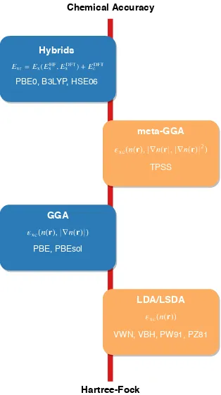
Figure 1.1 Example of Jacob’s ladder, with the general trend in accuracy of the
various DFT functionals. Beginning with Hartree-Fock, which in-cludes zero correlation, we increase the accuracy of the exchange and correlation as we move up from LDA and GGAs, into meta-GGAs and hybrid functionals. This is not true for every system, but is gen-erally accepted to be a reasonable description on the accuracy of the various density functionals. . . 13
Figure 2.1 Percent of correlation energy gained from QMC methods.
Hartree-Fock, by definition, neglects correlation energy. A single Slater
De-terminant with Jastrow trial wave function will typically gain∼80 %
correlation energy within VMC, and can achieve∼95 % using DMC. 30
Figure 2.2 Visualization of DMC algorithm for the ground state of the 1D
Har-monic Oscillator. The initial wave function is uniformly distributed.
After performing the diffusion and birth/death process, we arrive at
the long-time evolution already at 2 a.u., which is beginning to re-semble the normal distribution, i.e. the ground state of the Harmonic Oscillator. We only show a subset of the walkers, which is not neces-sarily representative of the final distribution. The final distribution is shown in the third panel. . . 33
Figure 2.3 Visualization of the Fermion Sign Problem in DMC. An initial set
of walkers is initialized into each sign region ofΨ, becoming two
independent distributionsΨ+andΨ−, each weighted by their sign.
As the simulation evolves to large times, each one independently arrives at the ground state distribution. Since each distribution is now weighted equally, but opposite in sign, they cancel and the fermionic signal is lost. . . 35
Figure 2.4 Visualization of a hypothetical nodal surface. The trial nodal surface,
∂ΩT, separates the configuration space into positive regions and
negative regions,Ω+T andΩ−
T respectively. The trial nodal surface is
intended to be as close as possible to the exact nodal surface∂Ω0. . . 37
Figure 3.1 Total energies of the lowest states of Pb atom from the FCI method
(cir-cles) with cc-pVnZ basis sets compared to FPSODMC with a COSCI
Figure 3.2 Total energies of the lowest states of Bi atom from CISDT (circles)
with cc-pVnZ basis sets compared to FPSODMC with COSCI
(long-dashed lines) and CISDT (short-(long-dashed lines) trial wave functions. The valence space include only 6s and 6p states. . . 47
Figure 4.1 Total energy of the Pb ground state. The “No Drift” and “Drift”
calcu-lations are indistinguishable at this scale. . . 58
Figure 4.2 Total energies of the Pb ground state with COSCI trial wave function.
The calculations were performed with drift,vS
D 6=0, and excluding
drift,vS
D=0 . . . 58
Figure 4.3 Total energy using COSCI and CISDT trial wave functions for the Pb
ground state. FCI with cc-VQZ and a CBS extrapolation are included as a reference. . . 59
Figure 4.4 Binding Curve of the Sn2molecule using averaged spin-orbit AREP
with FNDMC and spin-orbit REP with FPSODMC methods. The curves
are offset to dissociation limit 2E0(Sn)within each method to enable
comparison for the predicted binding energy of each method with experiment. . . 60
Figure 4.5 Binding curve of the Sn2molecule using large- and small-core REP.
The large- and small-core systems have 8 and 44 valence electrons, respectively. . . 60
Figure 5.1 Nodal surfaces forψT
C for various distortion parameters. The exact
nodal surface is shown in (a). Note that (b) is plotted with x,y,z
from−10 to 10 a.u. whereas (c) is plotted from−2.5 to 2.5 a.u. The
distortion is more localized at the origin for largerβ. . . 69
Figure 5.2 Total energy of the Li atom using the fixed-node method (FNDMC,
constant full line), with error bar interval (dashed lines), compared with the fixed-phase, complex wave function (FPSODMC) formula-tion a funcformula-tion of the time step for the degrees of freedom. The spatial
coordinates were evolved with a time stepτspatial=0.001 a.u. Further
details are explained in the text. . . 75
Figure 6.1 FPDMC energy of the C atom with varying spin massesµs (or
equiva-lently the spin time stepτs =τ/µs). The initial spin configurations
were chosen so that the wave function decomposes into a product of determinants. . . 83
Figure 6.2 Percentage error of the correlation energies in the fixed-node (FN)
Figure 6.3 Total energies for the Be atom with a two-configuration wave function.
The topxaxis shows the actual spin time step for the FN calculation,
which is linearly extrapolated to zero time step with an energy of
−14.66071(5)Ha. The bottomx axis indicates the spin mass for the
FP calculation, where with each value configurations are initialized
such thats1=s3=s ands2=s4=s0. We hold the spatial time step
fixed atτ=0.001 Ha−1throughout. . . 84
Figure 6.4 N2binding curve for the1Σgmolecular state using a HF nodal surface
or phase. The horizontal line indicates the experimental dissociation energy. The experimental error bar is too small to be visible on this scale. The small increase in FP underbinding comes from a slightly smaller fixed-phase bias in the N atom and a slightly larger bias in the dimer with the HF phase. We note that the results need not to be necessarily identical for Hamiltonians with ECPs due to marginal differences in localization errors from two close, but nonidentical trial wave functions. . . 84
Figure 7.1 FPSODMC total energies as a function of spin massµs for the lowest
spin-orbit split state in the3Σand5Πsymmetries. As one moves from
larger spin mass, the expectation value becomes that of the original
spin-orbit Hamiltonian, which shows that the3Σstate is the ground
state. . . 91
Figure 7.2 COSCI energies for theδx2−y2δx y active space. For the AREP
calcu-lations, the valence configurations are given for each level. The first level (3Σ) is 3-fold degenerate, whereas the second and third levels are 2- and 1- fold degenerate, respectively. Gaps relative to the ground state for each level are given for both AREP and REP calculations. Additionally, the overall energy shift by including the SO interaction is given as∆SO. . . 92
Figure 7.3 The difference in the charge density between DHF and PBE0 trial
wave functions for the outermost spinorsπ4σ2
z2σ2sδ4. In red, we show
where the PBE0 has a greater charge density. The black spheres in-dicate the location of the Tungsten atoms. (For interpretation of the references to colour in this figure legend, the reader is referred to the Web version of this article.) . . . 93
Figure 8.1 Boron dimer potential energy surface. UC represents an all-electron
CCSD(T) calculation with a self-consistent butuncorrelatedcore, i.e.,
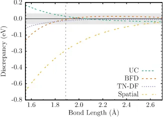
Figure 8.2 Boron dimer binding energy discrepancies compared to the all-electron CCSD(T) binding curve. The gray envelope represents a 0.05 eV win-dow for the discrepancy. The vertical line indicates the equilibrium bond length as predicted by the all-electron CCSD(T) calculation. . . 101
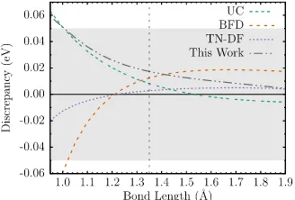
Figure 8.3 Carbon dimer binding energy discrepancies compared to the
all-electron CCSD(T) binding curve. . . 102
Figure 8.4 Nitrogen dimer binding energy discrepancies compared to the
all-electron CCSD(T) binding curve. . . 103
Figure 8.5 Oxygen dimer binding energy discrepancies compared to the
all-electron CCSD(T) binding curve. . . 104
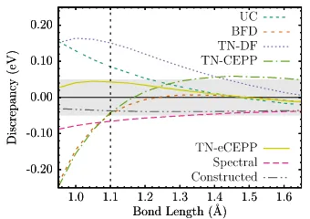
Figure 8.6 Potential energy surfaces of the S2molecule from CCSD(T). We have
plotted the predictions from various treatments of the sulfur cores. Shown are the all-electron (AE) core, all-electron uncorrelated core (UC), Burkatzki-Filippi-Dolg (BFD), Dirac-Fock Trail-Needs (TN) and the CCSD(T) spectrum matched (Spectral) ECPs described in the text. 105
Figure 8.7 Sulfur dimer binding curve energy discrepancies compared to the
all-electron CCSD(T) binding curve. . . 105
Figure 8.8 Sulfur dimer binding energy discrepancies compared to the all-electron
CCSD(T) binding curve. . . 105
Figure 8.9 NH binding energy discrepancies for various ECPs. . . 106
Figure 8.10 OH binding energy discrepancies for various ECPs. For oxygen, we use our spectral ECP. . . 106 Figure 8.11 NO binding energy discrepancies for various ECPs. For nitrogen, we
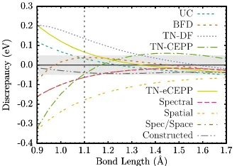
use our constructed ECP, and for oxygen, we use our spectral ECP. . . 106 Figure 8.12 SH binding energy discrepancies compared to the all-electron CCSD(T)
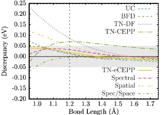
binding curve. For sulfur, we use our constructed ECP, and for oxygen, we use our spectral ECP. . . 106 Figure 8.13 SO binding energy discrepancies compared to the all-electron CCSD(T)
binding curve. For sulfur, we use our constructed ECP. . . 106 Figure 8.14 Discrepancies of molecular binding parameters of our ECPs, UC, and
previous constructions with respect to all-electron CCSD(T) calcula-tions. Parameters were obtained from Morse potential fits in all cases. (a) Dissociation energy discrepancies. (b) Equilibrium bond length
discrepancies. (c) Vibrational frequency discrepancies. . . 107
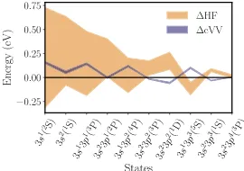
Figure 9.1 For the silicon atom, the spread of CCSD(T) valence-valence
cor-relation errors (∆cVV) and spread of HF errors (∆HF) for various
Figure 9.2 For the phosphorus atom, the spread of CCSD(T) valence-valence
correlation errors (∆cVV) and spread of HF errors (∆HF) for various
excitation energies from a variety of previously tabulated ECPs, in particular, BFD19, CRENBL21, SBKJC22, STU23, and TN-DF24. . . 113
Figure 9.3 Binding energy discrepancies for (a) Na2 and (b) NaO molecules
in their ground states1Σg and2Σ, respectively. The binding curves
are relative to the AE UCCSD(T) binding curve. The shaded region indicates a discrepancy of chemical accuracy in either direction. . . . 119
Figure 9.4 Binding energy discrepancies for the MgO molecule in its ground
state1Σ+.The binding curves are relative to the AE UCCSD(T)
bind-ing curve. The shaded region indicates a discrepancy of chemical accuracy in either direction. . . 120
Figure 9.5 Binding energy discrepancies for (a) Al2and (b) AlO molecules in their
ground states3Σg and2Σ, respectively. The binding curves are relative to the AE UCCSD(T) binding curve. The shaded region indicates a discrepancy of chemical accuracy in either direction. . . 120
Figure 9.6 Binding energy discrepancies for (a) Si2and (b) SiO molecules in their
ground states3Σg and1Σ, respectively. The binding curves are relative to the AE UCCSD(T) binding curve. The shaded region indicates a discrepancy of chemical accuracy in either direction. . . 120
Figure 9.7 Binding energy discrepancies for (a) P2and (b) PO molecules in their
ground states1Σgand2Π, respectively. The binding curves are relative to the AE UCCSD(T) binding curve. The shaded region indicates a discrepancy of chemical accuracy in either direction. . . 121
Figure 9.8 Binding energy discrepancies for (a) S2and (b) SO molecules in their
ground states3Σgand3Π, respectively. The binding curves are relative to the AE UCCSD(T) binding curve. The shaded region indicates a discrepancy of chemical accuracy in either direction. . . 121
Figure 9.9 Binding energy discrepancies for (a) Cl2and (b) ClO molecules in their
ground states1Σgand2Π, respectively. The binding curves are relative to the AE UCCSD(T) binding curve. The shaded region indicates a discrepancy of chemical accuracy in either direction. . . 121
Figure 9.10 Binding energy discrepancies for the ArH+molecule in its ground
state1Σ. The binding curves are relative to the AE UCCSD(T)
bind-ing curve. The shaded region indicates a discrepancy of chemical accuracy in either direction. . . 122
Figure 10.1 Spread of the contributions to the excitation energy for a variety
of ECPs compared to all-electron for the Fe atom.∆HF shows the
variation in the HF errors, whereas∆cVV shows the variation in the
Figure 10.2 Discrepancies for the various core approximations compared to all-electron CCSD(T) for select states. Each state discrepancy uses the
neutrals2dnoccupation as the reference, which is the neutral ground
state for each transition metal except for Cr and Cu, which haves1d5
ands1d10 ground states correspondingly. (a) The neutrals2dn →
s1dn+1 excitation. (b) The neutrals2dn →dn+2, (c) the ionization froms2dn → s1dn, and (d) the ionization from s2dn →[Ar]. The
shaded grap window in each figure indicates a discrepancy of half of chemical accuracy in either direction from the all-electron reference. We note that for Sc and Ti, our final ccECP is equivalent to our spectral ccECP.S. . . 133 Figure 10.3 Mean Absolute Deviation, or MAD, for the TMs considering a large
part of the spectrum from[Ar]up to low-lying neutral excited states
and the anion. The shaded region of half of chemical accuracy is not visible on the scale. We note that for Sc and Ti, our final ccECP is equivalent to our spectral ccECP.S. . . 133 Figure 10.4 Binding energy discrepancies for (a) ScH and (b) ScO molecules. The
binding curves are relative to the AE CCSD(T) binding curve. The shaded region indicates a discrepancy of chemical accuracy in either direction. . . 134 Figure 10.5 Binding energy discrepancies for (a) TiH and (b) TiO molecules. The
binding curves are relative to the AE CCSD(T) binding curve. The shaded region indicates a discrepancy of chemical accuracy in either direction. . . 135 Figure 10.6 Binding energy discrepancies for (a) VH and (b) VO molecules. The
binding curves are relative to the AE CCSD(T) binding curve. The shaded region indicates a discrepancy of chemical accuracy in either direction. . . 135 Figure 10.7 Binding energy discrepancies for (a) CrH and (b) CrO molecules. The
binding curves are relative to the AE CCSD(T) binding curve. The shaded region indicates a discrepancy of chemical accuracy in either direction. . . 136 Figure 10.8 Binding energy discrepancies for (a) MnH and (b) MnO molecules.
The binding curves are relative to the AE CCSD(T) binding curve. The shaded region indicates a discrepancy of chemical accuracy in either direction. . . 136 Figure 10.9 Binding energy discrepancies for (a) FeH and (b) FeO molecules. The
Figure 10.10 Binding energy discrepancies for (a) CoH and (b) CoO molecules. The binding curves are relative to the AE CCSD(T) binding curve. The shaded region indicates a discrepancy of chemical accuracy in either direction. . . 137 Figure 10.11 Binding energy discrepancies for (a) NiH and (b) NiO molecules. The
binding curves are relative to the AE CCSD(T) binding curve. The shaded region indicates a discrepancy of chemical accuracy in either direction. . . 137 Figure 10.12 Binding energy discrepancies for (a) CuH and (b) CuO molecules.
The binding curves are relative to the AE CCSD(T) binding curve. The shaded region indicates a discrepancy of chemical accuracy in either direction. . . 138 Figure 10.13 Binding energy discrepancies for (a) ZnH and (b) ZnO molecules. The
binding curves are relative to the AE CCSD(T) binding curve. The shaded region indicates a discrepancy of chemical accuracy in either direction. . . 138
Figure 11.1 LaScO3in the experimental perovskite structure. ScO6octahedra are
shown in purple, with the O atoms shown in red. The La+3cations are
shown in green. This figure was generated using the VESTA software [MI11]. . . 144
Figure 11.2 Mean-field bandstructures of LaScO3in the experimental structure.
(a) Hartree-Fock bandstructure, which has an indirect gap of 14.82 eV
with the VBM atΓ. The CBM is relatively flat around Γ. (b)
PBE0-25 bandstructure, which shows a direct gap atΓ of 6.51 eV. (c) PBE
bandstructure, which shows a direct gap atΓ of 4.04 eV. . . 148
Figure 11.3 FNDMC energies of the ground and excited states of LaScO3at theΓ
point using various ECPs. (11.3a) uses the ccECP for Sc and O, and the Rappe potential for La. (11.3b) uses the potentials designed for
QMC[Kro16]. The total energies are shown as a function of the nodal
surface generated from PBE0-αorbitals, whereαis the fraction of
CHAPTER
1
INTRODUCTION
From the 1800s to the early 1900s, a number of experiments led physicists to fundamentally change the way we view nature. With Young’s double slit experiment, the discovery of the electron with cathode ray tubes, and Millikan’s oil-drop experiment to name a few, the realization that microscopic phenomena is quantized led to quantum theory, a fundamental divergence from classical physics emerged full of seemingly counter-intuitive ideas like the wave-particle duality and the uncertainty principle. Nevertheless, these ideas are critical to our understanding of the natural world, from the biochemistry that drives life to solid-state physics description of semi-conductors that has fundamentally changed our modern world.
1.1
Many-body Schrödinger Equation
Electronic structure is focused on solving the many-body Schrödinger equation for electrons and nuclei. The Hamiltonian encodes all interactions between the individual particles, as well as their kinetic energies. We can write down the general Hamiltonian as
H = − ħh
2 2me
Ne X
i=1 ∇2i −
NI X
I=1
ħ
h2 2mI
∇2I
+1
2
NI X
I6=J
ZIZJe2
4πε0|rI −rJ|
−
Ne X
i=1
NI X
I=1
ZIe2
4πε0|ri−rI|
+1
2
Ne X
i6=j
e2 4πε0|ri−rj|
, (1.1)
whereNe is the number of electrons,NI is the number of ions, andm indicates the mass
of the particle. The first line contains the kinetic energies of all electrons and ions, the second contains the Coulomb repulsion between the individual ions as well as the Coulomb attraction between the ions and electrons, and the last line contains the electron-electron repulsion. In general, a solution to the electronic structure problem will amount to solving the time-dependent Schrödinger equation (TDSE)
iħh∂tΨ(R,t) =HΨ(R,t), (1.2)
where we have introduced the many-body wave function Ψ(R,t). Note thatRis a
high-dimensional vector containing all particle coordinates. Since our Hamiltonian does not explicitly depend on time, it is enough to solve the time-independent Schrödinger equation (TISE)
HΨn(R) =EnΨn(R), (1.3)
which allows one to discover the many-body spectrum{En,Ψn(R)}. By solving for a subset
of the many-body spectrum, a wide variety of properties can be obtained including
cohe-sion/binding, reaction barriers, optical properties, magnetic properties, structural phase
transitions, etc.
me <<mI for all ions. This implies that the kinetic energy of the ions is small, and move
much more slowly than the electrons in the system. Thus, we treat the ions as static with respect to the electrons, yielding in atomic units
Hel=−1 2
Ne X
i=1 ∇2i−
Ne X
i=1
NI X
I=1 ZI
|ri−rI|+ 1 2
Ne X
i6=j
1
|ri−rj|+Eion−ion. (1.4)
The solution for the electronic wave functions now depends parametrically on the ionic
coordinates. This is known as the Born-Oppenheimer (BO) approximation[BO27], which
allows us to define our system by the geometry of the ions, and then solve the TISE for the electronic wave function. In order to study bond dissociations, structural phase tran-sitions, phonon modes, etc., we only need to change the ionic coordinates and solve for the new electronic wave function. However, in studying phenomena such as electron-phonon coupling, which is thought to be a fundamental component of superconductivity
[Bar57a; Bar57b], explicit methods must consider the full Hamiltonian and solve for the full
electron-ion system. In all cases throughout this work, the BO approximation is sufficient to understand the electronic properties of various forms of matter. For the rest of this thesis, we will only be considering the electronic Hamiltonian given in Eqn. (1.4).
1.2
The Hartree-Fock Method
The Hartree-Fock (HF) method is the simplest approximation to the many-body wave function, which satisfies the observation that fermionic states need to be antisymmetric with respect to the exchange of electrons, colloquially known as the Pauli exclusion principle. The HF wave function is often used as a starting point for more sophisticated methods, such as configuration interaction (CI), coupled-cluster (CC), and Slater-Jastrow wave functions in quantum Monte Carlo (QMC). Due to its ubiquitous use throughout the quantum chemistry and solid state community, we review the method here. For a more complete survey, see
Modern Quantum Chemistryby Szabo and Ostlund[SO96].
The Hartree-Fock method relies on the variational theorem in quantum mechanics, which provides a framework for systematically improving a trial wave function. Given a
trial wave function|ΨT〉, we can always expand it into a complete basis, in particular the
function, we can insert the eigenbasis expansions as
ET = P α,β
〈ΨT|α〉〈α|H|β〉〈β|ΨT〉
P
α〈ΨT|α〉〈α|ΨT〉 =
P α |cα|
2E α
P α |cα|
2 . (1.5)
We can always normalize the trial wave function, in which the denominator is unity. The numerator is over the entire many-body spectrum. Since the spectrum of the many-body Hamiltonian has a lower bound, i.e., a ground stateE0<E1<. . ., it is clear that if|ΨT〉is
not orthogonal to the ground state, then we have the condition thatET ≥E0. Therefore,
the trial energy is always bounded from below by the exact energy. The existence of a
variational theorem allows us to optimize a given functional form of|ΨT〉to find the optimal
approximate wave function. The Hartree-Fock wave function can be obtained using these arguments.
To construct the HF wave function, we first consider the case of fully non-interacting
distinguishablequantum particles, with a HamiltonianH =P
ihi, wherehi is a
single-particle Hamiltonian. Each individual single-particle will occupy as single-single-particle wave function, or spin-orbital, which is an eigenstate of the single particle Hamiltonian,hiψj(ri) =εjψj(ri).
In this non-interacting case, the many-body wave function can be constructed as a product of the single-particle orbitals, otherwise known as the Hartree product
Ψ(x1, . . . ,xN) = N Y
i=1
ψi(xi), (1.6)
wherexi = (ri,si)are the particle coordinates of space ri and spinsi for particlei. For
fermions, we must include the antisymmetry of the wave function, namely under exchange of particle coordinates we must pick up a sign, namely
Ψ(x1, . . . ,xi, . . .xj, . . .xN) =−Ψ(x1, . . . ,xj, . . . ,xi, . . . ,xN). (1.7)
It is well known that the determinant satisfies this contraint and changes sign under
ex-change of rows/columns in the matrix. Therefore, the simplest ansantz will be to treat the
function is antisymmetric. This ansatz is known as the Slater determinant, and is given by
Ψ(x1, . . . ,xN) = p1 N!
ψ1(x1) . . . ψ1(xN) ψ2(x1) . . . ψ2(xN)
..
. ... ...
ψN(x1) . . . ψN(xN)
= p1
N!
N!
X
n=1
(−1)pnPˆ n
ψ1(x1). . .ψN(xN), (1.8)
where the Slater determinant is normalized by p1
N!assuming orthonormal spin-orbitals,
and ˆPn is a permutation operator on the particle coordinates. Since there areN particles,
there areN! possible permutations to ensure indistinguishability. In order to derive the
Hartree-Fock equations, we must first know the expectation value of the Slater determinant with the Hamiltonian. If we write our Hamiltonian as a sum of one- and two-body operators, H =Pihi+12
P
i6=jri j−1, we must evaluate
〈Ψ(X)|H|Ψ(X)〉 = N〈Ψ(X)|h1|Ψ(X)〉+N(N −1)
2 〈Ψ(X)|r
−1
12|Ψ(X)〉. (1.9)
Since the particles are indistinguishable, we only need to evaluate the one- and two-body
operators for a single particle/pair, and multiply it by the number of particles/pairs. We
assume the Slater determinant is normalized so we can ignore the denominator in the expectation value. The one-body operators, which contain the kinetic energy and the electron-ion interaction, can be reduced to a sum over matrix elements of the orbitals
N〈Ψ(X)|h1|Ψ(X)〉 = N N!
N!
X
n=1,m=1
(−1)pn+pm Z
dXPˆm
ψ∗
1(x1). . .ψ
∗ N(xN)
h1Pˆn
ψ1(x1). . .ψN(xN)
= 1
(N−1)!
N!
X
n=1
Z
dx1. . . dxNPˆn
ψ∗
1(x1). . .ψ
∗ N(xN)
h1Pˆn
ψ1(x1). . .ψN(xN)
= N X
i=1
Z
dx1ψ∗i(x1)h1ψi(x1) =
N X
i=1
〈ψi|h1|ψi〉, (1.10)
where we assume that the orbitals are orthonormal, i.e.,〈ψi|ψj〉=δi j. The second line
is canceled by the fact that there are(N−1)! ways to organize particles 2 throughN. The two-body matrix elements proceed in a similar fashion, except that the key difference is that electrons 1 and 2 have two different permutations. Taking this into account, we obtain for the two-body matrix elements
N(N−1)
2 〈Ψ(X)|r
−1
12 |Ψ(X)〉 = 1 2
N P i6=j R
dx1dx2ψ∗i(x1)ψ∗j(x2)r12−1
ψi(x1)ψj(x2)−ψj(x1)ψi(x2)
=1
2
N P i6=j
〈ψiψj|r12−1|ψiψj〉 − 〈ψiψj|r12−1|ψjψi〉, (1.11)
where the first term is the direct (classical) coulomb interaction between the two electrons,
and the second is a purely quantum mechanical interaction known asexchangewhich
comes from the requirement of antisymmetry in the fermionic wave function.
From Eqn. (1.10) and (1.11), we can construct the full expectation value for a single Slater determinant. In order to invoke the variational principle, we want to minimize this expectation value while maintaining this simple determinant form, i.e. optimizing the orbitals themselves. We can achieve this by minimizing the variational energy subject to the constraint that the orbitals remain orthonormal utilizing the method of Lagrange multipliers. We minimize the functional
L[{ψi}] =〈Ψ[{ψi}]|H|Ψ[{ψi}]〉 − N X
i=1,j=1
εi j(〈ψi|ψj〉 −δi j)
= N X
i=1
〈ψi|h1|ψi〉+
1 2
N X
i,j=1
〈ψiψj|r12−1(1−Pˆ12)|ψiψj〉 − N X
i,j=1
εi j(〈ψi|ψj〉 −δi j), (1.12)
where we no longer restrict the sum since the expectation value for the two-body operator vanishes ifi=j due to the presence of exchange. We take the first variation in the functional above and set it to zero. Since the variation will be applied to both the bras and kets on each expectation value, we recognize that the entire variation becomes
δL =
N X
i=1
〈δψi|h1|ψi〉+
1 2
N X
i,j=1
〈δψiψj|r12−1|ψiψj〉 − 〈δψiψj|r12−1|ψjψi〉
−
N X
i,j=1
Since the variation in the orbital is arbitrary, the rest of the expression must vanish. If one further considers the unitary invariance of the Slater determinant, the canonical Hartree-Fock expression is obtained
h1+
N X
j=1
Z
dx2ψ∗j(x2)r12−1 1−Pˆ12
ψj(x2)
ψi(x1) = εiψi(x1)
ˆ
fψi(x1) = εiψi(x1), (1.14)
where ˆf is the Fock operator. This takes the form of an eigenvalue equation and the optimal
orbitals are then obtained self-consistently. In practice, these orbitals are expanded in a (finite) basis set
ψi(x) = Nb X
k
bi kfk(x), (1.15)
where the basis functions fk can be any function, typically chosen such that the evaluation
of the orbital is fast and efficient. The most common choices are localized gaussians and
delocalized plane waves. Choosing a particular basis set sizeNb will generateNb orbitals
within Hartree-Fock. The lowestNe will be occupied orbitals within the Slater determinant
to form the ground state, and the remaining unoccupied orbitals are known as virtual or-bitals. As the basis set becomes complete, the Hartree-Fock energy for the basis approaches the exact Hartree-Fock limit. The introduction of the basis set turns Eqn. (1.14) into a matrix equation
FC=εSC, (1.16)
whereFis the Fock matrix,Care the eigenvectors (orbitals),ε is the eigenvalue matrix
(orbital energies), andSis the overlap matrix of the orbitals. Although the Hartree-Fock
expressions above are given for open boundary conditions, we can generalize the expres-sions for periodic boundary conditions given a periodic potential following Bloch’s theorem
[Blo29]. By generalizing the basis functions into Bloch functions
fi(x,k) = X
G
eik·Gfi(x−G)≡eik·rui(r,k), (1.17)
the Hartree-Fock expressions for periodic systems[Dov; McC17]
FkCk=εkSkCk. (1.18)
By solving the above equations, either in open or periodic boundary conditions, we obtain the simplest description of the electrons in the system which properly accounts for their anti-symmetry.
The exact/complete basis Hartree-Fock energy is the lowest variational energy that
is generated from the simplest fermionic wave function, EHF. This differs from the exact
ground state energy,E0, by an amount known as thecorrelation energy
Ecorr=E0−EHF. (1.19)
The correlation energy is typically very small on the scale of the total energy, on the order of a few percent. However, the correlation energy typically on the same order as the relevant
properties of the system, such as cohesion/binding or fundamental/optical gaps of the
material. For example, cohesive energies of solids at the HF level can be in error of roughly
50%[Fou01]. Therefore, an accurate treatment of correlations is crucial to describe both
chemistry and solid state phenomena. One option in treating these correlations is to turn to other wave function based methods that build upon HF as a reference, known as post-HF methods.
1.3
Post Hartree-Fock Methods
Wave function based improvements to Hartree-Fock are all based on wave function expan-sions in Slater determinants. Formally, the space of Slater determinants forms a complete basis, therefore the exact wave function can be expanded as
|Ψ〉=d0|ΨHF〉+
X
α,θ
dα→θcˆθ†cˆα|ΨHF〉+
X
α,β,θ,ω
dα→θ,β→ωcˆθ†cˆω†cˆβcˆα|ΨHF〉+. . . , (1.20)
where α,β indicate occupied orbitals, and θ,ω represent virtual orbitals, and the
cre-ation/annhilation operators ˆc†
basis set. The number of possible determinants can be determined by
Ndet=
Nb
Ne
, (1.21)
which is clearly exponentially scaling as the basis increases. Minimization of the energy
within this determinant space for a given basis are known asconfiguration interaction
(CI) methods. A number of different approaches exist for treating correlations in this way. The most straightforward is to simply truncate the expansion at a given excitation level like singles and doubles, known as CISD. In very limited cases, an exact full configuration interaction (FCI) can be used. More recent methods rely on stochastic and perturbative techniques to choose the relevant determinants this determinant space, such as selected CI
[Hol16a; Hur73]and FCIQMC[Boo09]. The CI methods described above directly utilize the
HF orbitals, and simply optimize the expansion coefficients. However, another approach is to directly optimize both the orbital set and the CI coefficients simultaneously while
maintaining orthonormality of the single particle orbitals is known asmulti-configurational
SCFor MCSCF.
The CI and MCSCF methods rely on linear wave function expansions, and thus clearly satisfy the variational principle. In fact, an alternative method known as Coupled Cluster
[C66ˇ ]uses an exponential ansatz for the wave function of the form
|ΨCC〉=e ˆ
T
|Ψref〉, (1.22)
where the reference state is typically chosen as the HF wave function,|Ψref〉=|ΨHF〉. The
exponential operator generates various levels of particle excitations, which is typically truncated at doubles, ˆT =Tˆ1+Tˆ2, although higher orders are in principle possible. The ˆT1 and ˆT2operators are written in terms of the creation/annhilation operators in Eqn. (1.20) as
ˆ
T1 =
X
α,θ
tα(1→)θcˆθ†cˆα
ˆ
T2 =
X
α,β,θ,ω
tα(2→)θ,β→ωcˆθ†cˆω†cˆβcˆα. (1.23)
Triple excitations are often included perturbationally, known as CCSD(T) and is often
considered the “gold standard” of quantum chemistry[BM07], but due to the poor scaling
which makes higher order truncation feasible in both memory and cost, but this ultimately still scales too poorly to generalize to arbitrary system sizes. Coupled Cluster has also been
developed for periodic systems[McC17], but is restricted to small primitive cells and basis
sets. It is therefore desirable to find a many-body method to treat electronic correlations that scales more favorably with system size.
1.4
Density Functional Theory
As an alternative to the wave function based methods described previously, the Schrödinger equation can also be dealt with by directly working with the density. In wave function based methods, the strategy is to define the external potential for the system, solve the Schrödinger equation for the many-body wave function, and calculate any desired observables from this. The Hamiltonian is uniquely defined by the external potential, since the kinetic energy and electron-electron interaction are always present. The electron density is an observable
found from this many-body wave function. The density operator is given as ˆn=
N P i=1
δ(r−ri), therefore the electron density is
n(x) =〈Ψ|nˆ|Ψ〉 =
N X
i=1
Z
dRΨ∗(R)δ(r−ri)Ψ(R)
= N
Z
dr2. . . drNΨ∗(r,r2, . . . ,rN)Ψ(r,r2, . . . ,rN) (1.24)
assumingΨ(R)is normalized.
In Density Functional Theory (DFT), the density becomes the fundamental quantity as opposed to the wave function. The realization that properties of many-body systems can
be expressed as a functional of the density was first shown by Hohenburg and Kohn[HK64].
Their theorems and some consequences can be summarized as follows[Cap06],
• The exact ground state wave function,Ψ0(R), of a given system is afunctionalof the exact ground state density,n0(r), i.e.
• The ground state energy is a functional of the ground state density
E0[n0(r)] =〈Ψ0[n0(r)]|H|Ψ0[n0(r)]〉 (1.26)
and is variational, i.e.E0[n0]≤E[n0], wheren0is a different density. Similarly, any
ground state expectation values can be formulated by replacing the Hamiltonian with the appropriate operator. Therefore all ground state observables are functionals of the ground state density, i.e.
O0=O[n0] =〈Ψ[n0]|Oˆ|Ψ[n0]〉. (1.27)
• We can write a general energy functional as
E [n(r)] =T [n] +Ve e[n] +Vext[n] =F[n] +Vext[n], (1.28)
whose global minimum is the ground state energy. The kinetic energy and electron-electron interaction are universal functionals, and are the same for every electron-electronic system. The external potential, when held fixed is not universal, and is specific to the system under consideration. The external potential functional is given as
Vext[n(r)] =
Z
drn(r)Vext(r). (1.29)
• If the external potential is not held fixed, the external potential functional is also universal. Therefore, the density uniquely determines the external potential (up to a constant). From this, the Hamiltonian is fully determined and thus all excited states are determined, in principle, from only the ground state density.
The Hohenberg-Kohn theorems are straightforward to prove[Mar04], and can be found in
their original work as well as alternative formulations by Levy and Lieb[Lev82; Lie83]. The Hohenberg-Kohn theorems show that the density can be viewed as a fundamental quantity, and in principle is sufficient to describe the many-body system and its observables. In practice, they do not provide a method for obtaining this density. The Kohn-Sham ansatz makes DFT a practical method by replacing the fully interacting many-body problem with
is equal to the density of an independent particle system, i.e.
nKS(r) =
N X
i=1
ψi,KS(r)
2
=〈Ψ0|nˆ|Ψ0〉=n0(r), (1.30)
whereψi,KS(r)
N
i=1are the Kohn-Sham non-interacting orbitals. Since we are assuming the
many-body density can be written in terms of the density of some independent auxillary particles, we can consider their kinetic energy and classical Coulomb (Hartree) functionals,
TKS[n] = − 1 2
N X
i=1
Z
drψ∗i,KS(r)∇2ψi,KS(r) (1.31)
EHartree[n] = 1 2
Z
drdr0nKS(r)nKS(r
0)
|r−r0| . (1.32)
Under this assumption, we can rewrite the Hohenberg-Kohn functional in Eqn. (1.28) as
E[n] = 〈Ψ[n]|T +Vee|Ψ[n]〉+Vext[n]
= TKS[n] +EHartree[n]−(TKS[n] +EHartree[n]) +〈Ψ[n]|T +Vee|Ψ[n]〉+Vext[n]
= TKS[n] +EHartree[n] +Vext[n] +Exc[n], (1.33)
where we have defined a new functional, known as theexchange-correlationfunctional as
Exc[n] =〈Ψ|T +Vee|Ψ〉 −TKS[n]−EHartree[n]. (1.34)
The exchange-correlation functionalEx c contains all of the many-body interaction
LDA/LSDA VWN, VBH, PW91, PZ81
( ( )) xc
GGA PBE, PBEsol
( ( ), |∇ ( )|) xc
meta-GGA TPSS
( ( ), |∇ ( |, |∇ ( ) )
xc |2
Hybrids PBE0, B3LYP, HSE06
= ( , ) + xc x xHF DFTx cDFT
Hartree-Fock Chemical Accuracy
Figure 1.1Example of Jacob’s ladder, with the general trend in accuracy of the various DFT
func-tionals. Beginning with Hartree-Fock, which includes zero correlation, we increase the accuracy of the exchange and correlation as we move up from LDA and GGAs, into meta-GGAs and hy-brid functionals. This is not true for every system, but is generally accepted to be a reasonable description on the accuracy of the various density functionals.
Hartree-Fock expressions, we obtain the Kohn-Sham equations
−1
2∇
2+V
e f f(r)
ψi,KS(r) = εi,KSψi,KS(r) (1.35)
Ve f f(r) = Vext(r) +
δEHartree
δn +
δExc
δn (1.36)
which can be solved self-consistently for the Kohn-Sham orbitals and energiesεi,KS. Similar
to the Hartree-Fock method, the solution to the Kohn-Sham equations can be facilitated by the use of basis sets.