FULL PAPER
Distribution and depth
of bottom-simulating reflectors in the Nankai
subduction margin
Akihiro Ohde
1,2*, Hironori Otsuka
3, Arata Kioka
4and Juichiro Ashi
1,2Abstract
Surface heat flow has been observed to be highly variable in the Nankai subduction margin. This study presents an investigation of local anomalies in surface heat flows on the undulating seafloor in the Nankai subduction margin. We estimate the heat flows from bottom-simulating reflectors (BSRs) marking the lower boundaries of the methane hydrate stability zone and evaluate topographic effects on heat flow via two-dimensional thermal modeling. BSRs have been used to estimate heat flows based on the known stability characteristics of methane hydrates under low-temperature and high-pressure conditions. First, we generate an extensive map of the distribution and subseafloor depths of the BSRs in the Nankai subduction margin. We confirm that BSRs exist at the toe of the accretionary prism and the trough floor of the offshore Tokai region, where BSRs had previously been thought to be absent. Second, we calculate the BSR-derived heat flow and evaluate the associated errors. We conclude that the total uncertainty of the BSR-derived heat flow should be within 25%, considering allowable ranges in the P-wave velocity, which influences the time-to-depth conversion of the BSR position in seismic images, the resultant geothermal gradient, and thermal resistance. Finally, we model a two-dimensional thermal structure by comparing the temperatures at the observed BSR depths with the calculated temperatures at the same depths. The thermal modeling reveals that most local vari-ations in BSR depth over the undulating seafloor can be explained by topographic effects. Those areas that cannot be explained by topographic effects can be mainly attributed to advective fluid flow, regional rapid sedimentation, or erosion. Our spatial distribution of heat flow data provides indispensable basic data for numerical studies of subduc-tion zone modeling to evaluate margin parallel age dependencies of subducting plates.
Keywords: Surface heat flow, Bottom-simulating reflector, Methane hydrate, Shallow thermal structure, Nankai Trough
© The Author(s) 2018. This article is distributed under the terms of the Creative Commons Attribution 4.0 International License (http://creativecommons.org/licenses/by/4.0/), which permits unrestricted use, distribution, and reproduction in any medium, provided you give appropriate credit to the original author(s) and the source, provide a link to the Creative Commons license, and indicate if changes were made.
Open Access
*Correspondence: [email protected]
1 Atmosphere and Ocean Research Institute, The University of Tokyo,
5-1-5 Kashiwanoha, Kashiwa, Chiba 277-8564, Japan
Full list of author information is available at the end of the article Introduction
The development of gas hydrates, the guest molecules consisting of almost pure methane (e.g., Kvenvolden 1988), has been confirmed in marine sediments using seismic reflectors, sediment cores, and downhole logging data (e.g., Shipley et al. 1979; Kvenvolden and McDon-ald 1985; Cook et al. 2010). The range in depth of the methane hydrates has been determined by subseafloor temperatures and pressures (e.g., Shipley et al. 1979;
Dickens and Quinby-Hunt 1994). Therefore, the presence of methane hydrate can be used to obtain subseafloor thermal information by taking advantage of the hydrate’s known stability characteristics under low-temperature and high-pressure conditions.
(BGHS), which is a phase boundary between the meth-ane hydrate and free gas. Therefore, many previous stud-ies have investigated the subseafloor thermal regime based on BSR characteristics (Yamano et al. 1982, 1984; Ashi et al. 2002; Harris et al. 2013). Hyndman and Wang (1993) provided constraints on the seismogenic zone with a thermal model that utilized heat flow values from BSR, probe, and borehole measurements.
The heat flow value is generally dependent on the age of the incoming plate (Stein and Stein 1992). The advection of the subducting plate results in substantially reduced heat flow from the margin wedge and forearc relative to the incoming plate. There are locally high or low heat flow observations superimposed on the regionally low heat flow on the wedge and forearc. These are thought to be mainly due to advective fluid flows (e.g., Wang et al. 1993, 1995), rapid sedimentation or erosion (Hutchison 1985; Wang et al. 1993), or fault activity (e.g., Kinoshita et al. 2011). In addition, topographic effects that arise in convex-upward and convex-downward topographies also cause locally high or low heat flows (Ganguly et al. 2000; Chen et al. 2014; Li et al. 2014). Identifying the phenom-ena that cause local high or low heat flows is important because surface measurements of heat flow are utilized to estimate thermal properties in plate subduction zones, including frictional strength along plate boundaries and radioactive heat production.
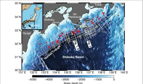
In the Nankai accretionary margin, BSRs are widely distributed through the accretionary prism and forearc basins (Aoki et al. 1982; Ashi et al. 2002; Baba and Yam-ada 2004; Otsuka et al. 2015). Therefore, heat flow can be acquired by thermistor probes and borehole meas-urements and by BSRs, which provide continuous heat flow profiles, unlike the instrumental measurements. In this study, we first investigate in detail the distribution of BSRs over the accretionary prism slope and the forearc basins, from offshore Tokai to Hyuga in the Nankai sub-duction margin (Fig. 1), using two-dimensional (2-D) multi-channel seismic (MCS) reflection data. We also compare the heat flow derived from BSRs with those esti-mated from probe and borehole measurements. Second, we estimate two-dimensional shallow thermal structures in the Nankai subduction margin that are constrained by temperatures at BSRs. This enables the discussion of fac-tors that influence local BSR depth anomalies in convex and concave topographies, which is the main purpose of our study. This method advances the understanding of the effects of past surface geological phenomena, such as prominent sedimentation or erosion.
Regional setting
Geological setting
The Nankai Trough, formed by the northwestward subduction of the Philippine Sea Plate (PHP in Fig. 1) beneath the Eurasian plate at approximately 4 cm/ year (e.g., Seno et al. 1993), is a plate boundary where earthquakes of magnitude 8 have occurred at intervals of 100–200 years (e.g., Satake 2015). Recent megath-rust earthquakes with magnitude classes of 8 in the Nankai subduction zone include the Tonankai earth-quake in 1944 and the Nankai earthearth-quake in 1946 (e.g., Kanamori 1972). The geological structure in the Nankai accretionary margin can be divided from the southeast to the northwest into a deformation front, a prism slope with slope basins, an outer ridge associ-ated with a megasplay fault, and a forearc basin. The Kumano Basin, one of the major forearc basins along the Nankai Trough, is approximately 100 km from east to west and approximately 70 km from north to south (Morita et al. 2004). The Nankai Trough is character-ized by a shallow trench due to the subduction of the young plate and contains thick trench-fill sediments at a water depth of approximately 4000 m ranging from south of Suruga Bay to the northern tip of the Kyushu-Palau Ridge.
Previous heat flow studies
Many previous studies estimated heat flow values using probes and BSRs in the Nankai Trough (e.g., Yamano et al. 1982). Heat flow values gradually decreased from the trough floor to the forearc basin, as Yamano et al. (2003) estimated through a heat flow probe. Although the heat flow values tended to decrease landward, as reported above, they were also found to vary with topog-raphy on a local scale, especially in convex-upward and convex-downward seafloor regions, as indicated by Gan-guly et al. (2000), who concluded that heat flow could increase by as much as 50% on an undulating seafloor. Harris et al. (2013) found broad agreement between the heat flow measured by probes and those derived from BSRs in the Nankai margin. Offshore Muroto (offshore southeast of Shikoku), high heat flow values of approxi-mately 200 mW/m2 were observed by probes in previous
Seismic data and BSR picking
The data for this study were derived from sixteen MCS reflection survey cruises by the research vessels (R/Vs) Kairei and Kaiyo (JAMSTEC, Japan), and the R/V Polar Princess (GC Rieber Shipping, Norway), for a total of 142 survey lines (Fig. 1). The seismic surveys referred to as KR9702 (acquired in 1997), KR9704 (1997), KR9806 (1998), KR9810 (1998), KR9904 (1999), KR0108 (2001), KR0114 (2001), KR0211 (2002), KR0413 (2004), KR0512 (2005), KR1011 (2010), KR1109 (2011), and KR1212 (2012) were conducted by the R/V Kairei; KY0314 (2003) and KY1311 (2013) were conducted by the R/V Kaiyo; and ODKMPP03 (2003) was conducted by the R/V Polar Princess. Data acquisitions from the KR9702, KR9704, KR9806, and KR9810 surveys were performed with an airgun array with a volume of ~ 66 L fired at 50-m inter-vals and a streamer with a length of ~ 3.5 km contain-ing 120 receivers. Data from KR9904, KR0108, KR0114, KR0211, and KY0314 were acquired with an airgun array
with a volume of ~ 200 L fired at 50-m intervals and a streamer with a length of ~ 4 km containing 156 receiv-ers. Data from KR0413 and KR0512 were obtained with an airgun array with a volume of ~ 200 L fired at 50-m intervals and a streamer with a length of ~ 5.5 km con-taining 204 receivers. Data from KR1011, KR1109, KR1212, and KY1311 were obtained with an airgun array with a volume of ~ 128 L fired at 50-m intervals and a streamer with a length of ~ 6 km containing 444 receiv-ers. Data from ODKMPP03 were acquired with an air-gun array with a volume of ~ 70 L fired at 50-m intervals and a streamer with a length of ~ 6 km containing 480 receivers.
All the MCS reflection data were processed conven-tionally with trace editing, common mid-point (CMP) sorting (with CMP intervals of 12.5 m for the seismic data acquired by the R/V Kairei and Kaiyo cruises com-pleted by 2005; 6.25 m for the data from the ODKMPP03, KR1011, KR1109, and KR1212 surveys; and 3.125 m
131˚E 132˚E 133˚E 134˚E 135˚E 136˚E 137˚E 138˚E 139˚E 140˚E
30˚N 31˚N 32˚N 33˚N 34˚N 35˚N
−5000 −4000 −3000 −2000 −1000 0
Water depth [m]
Nankai Trough
Kyushu−Palau
Ridg e
Kumano Basin
Embaymen
t A
B
Tokai
Kii Peninsula Shikoku
Hyuga
Muroto
Shikoku Basin
C0002 1946
1944
Fig. 2 Fig. 7,
9
4 cm/yr PHP
JAPAN
Fig. 1 Study area from offshore Tokai to Hyuga in the Nankai subduction margin. Gray lines represent the MCS reflection surveys studied in this
work. Yellow dots represent the locations of BSRs identified in Figs. 2, 6b, c. Red dots denote the locations used to calculate the thermal structure
via thermal modeling, which adopts the temperatures at the BSR depths as a constraint and, therefore, requires continuous BSRs (see Additional
file 1: Figures S2 and S3 for more detail on the modeling section, and Figures S4–S23 for modeling results). Black stars indicate the epicenters of the
Tonankai earthquake in 1944 and Nankai earthquake in 1946 (Kanamori 1972). Site C0002 of the IODP Expeditions (Expedition 314 Scientists 2009)
is indicated by a white star. Note that there are many other IODP wells where heat flows have been determined using borehole measurements (e.g.,
Harris et al. 2011; Marcaillou et al. 2012; Harris et al. 2013) (see Fig. 8a). The seismic profile of the A–B section is illustrated in Fig. 7, and the thermal
structure modeled over the section is shown in Fig. 9. The parameters used in the thermal modeling of the A–B section are shown in Table 2. A total
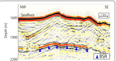
for the data from the KY1311 survey), band-pass filter-ing, gain, deconvolution, mutfilter-ing, velocity analysis, nor-mal moveout correction, CMP stacking, and post-stack time migration. The vertical resolution (Rayleigh’s crite-rion) within the dominant frequencies and studied time domains was 10–20 m. All processing, including imaging and BSR picking, was conducted using the commercial software, Paradigm Product Manager. In this study, the BSRs were carefully identified as distinct acoustic reflec-tors that displayed the characteristics of paralleling the seafloor based on seismic reflection images that exhibited high-amplitude reverse-polarity waveforms (Fig. 2).
Methods
Heat flow derived from BSR depth
Heat flow is generally measured through penetration of a 4.5–6.0-m probe with temperature sensors and occa-sionally via in situ borehole temperature measurements in deep-sea drilling. However, BSR depths constrained by the pressure–temperature conditions have also been used as an effective method for heat flow estimation (e.g., Yamano et al. 1982). Both the probe and BSR methods have advantages and disadvantages that are related to the regions of interest. In general, the probe method can measure heat flow values at any location where the probe can penetrate the seafloor, whereas the BSR method is restricted to areas where BSRs are present, such as con-tinental margins. In areas of bottom water temperature fluctuation, short thermal probes are more susceptible to uncertainties arising from these variations (Davis et al. 2003), unless the effect is removed through long-term observations of the bottom water temperature (Hama-moto et al. 2005). In contrast, values estimated from the
BSRs are less affected by the bottom water temperature variations because, in most areas, the BSR depths are located hundreds of meters below the seafloor. There-fore, the values calculated from the BSRs can be used to estimate the geothermal regime up to approximately 1 km below the seafloor. Moreover, because the presence of BSRs in the Nankai subduction zone has been widely confirmed (Ashi et al. 2002; Baba and Yamada 2004; Otsuka et al. 2015), heat flow values can be calculated over wide areas when physical properties, such as seismic velocity, density, and thermal resistance, are estimated from seismic surveys and deep-sea drilling.
In this study, we used the relationship between the two-way travel time and the depth obtained from the check shot survey at Site C0002 of the Integrated Ocean Drilling Program (IODP) Expedition 314 (Expedition 314 Scientists 2009) to convert the two-way travel time into depth in all MCS reflection images. The IODP Site C0002 was selected because many of our survey lines were densely distributed near IODP Site C0002 (Fig. 1) and because this site afforded the most reliable P-wave veloc-ity, including uncertainty, although some of our MCS reflection images were obtained farther away from the IODP site. The velocity in the overlying seawater column was assumed to be 1500 m/s.
We assumed hydrostatic pressure within the sediment columns above the BSRs; the differences in the results that arise from formation pressures between hydrostatic and lithostatic conditions were discussed in the follow-ing section. Usfollow-ing a phase diagram for methane hydrate (Tishchenko et al. 2005), the estimated pressure indicated the temperature at the BSR depth. Although other gases such as CO2 and H2S affect the phase boundary of
meth-ane hydrate (Claypool and Kaplan 1974), core samples revealed that methane hydrate in the Nankai subduction zone consists of almost pure methane (~ 99%) (Tobin et al. 2015).
The seafloor temperature was derived from the hydro-graphic data of the bottom water temperature from the Japan Oceanographic Data Center, which was then used in part to compute the geothermal gradient. The thermal conductivity of the formation between the seafloor and the BSR was estimated from shipboard measurements of discrete samples obtained at Site C0002 of IODP Expe-ditions 315 and 338 (Expedition 315 Scientists 2009; Strasser et al. 2014). Values of thermal conductivity cor-responding to the subseafloor depth were adopted. As the burial depth increased, sediment compaction occurs and porosity decreased. Consequently, the P-wave veloc-ity and thermal conductivveloc-ity increased with increasing burial depth. Therefore, integrated values of thermal resistance were adopted at depths between the seafloor Fig. 2 Example of BSR picking from the seismic profile generated by
the KR0211 cruise. The picked BSRs are marked with blue triangles; at these points, the seismic profiles exhibited the characteristic of high-amplitude reverse-polarity waveforms paralleling the seafloor compared with the seafloor reflector waveforms. The two-way travel time is converted to subseafloor depth using a P-wave velocity obtained from Site C0002 of the IODP Expeditions (Expedition 314
and the BSR. Finally, the heat flow was calculated from the geothermal gradient and the thermal resistance.
Uncertainty in BSR‑derived heat flow
When we converted the two-way travel time into depth and calculated thermal resistance, we applied the physi-cal properties from the sedimentary rocks at Site C0002 of the IODP Expeditions (Kinoshita et al. 2009) to the other BSR areas, allowing the heat flow values to be cal-culated wherever BSRs are recognized. However, errors may become large in cases where the physical properties of the sediment deviate greatly from those of the IODP Site C0002 (Kinoshita et al. 2009).
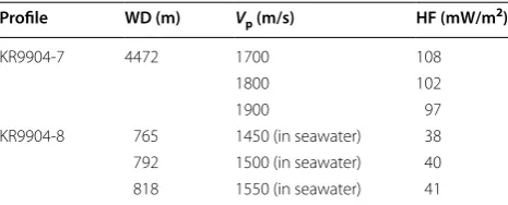
Determining heat flow from the BSRs involved trade-off relationships among several parameters (e.g., Greve-meyer and Villinger 2001) as discussed below. In this study, we conducted an error evaluation of the heat flow values by varying the P-wave velocity between 1700 and 1900 m/s based on the relationship between the two-way travel time and the depth obtained from IODP Site C0002 (Expedition 314 Scientists 2009) (Table 1) to account for this significant variation in the velocity in the sediment with the presence of different gases or porosi-ties. When we overestimated the P-wave velocity within the sequence above the BSR, the apparent BSR depths appeared deeper in the seismic reflection image, decreas-ing the geothermal gradient and the thermal resistance. Ultimately, a trade-off between underestimating the geo-thermal gradient and the geo-thermal resistance reduced the resulting heat flow variation. Moreover, we considered that the heat flow values were calculated using the physi-cal properties of the forearc basin at IODP Site C0002, which may differ from those of the prism slope. There-fore, we also evaluated the uncertainty using the physical properties of the prism slope at Site 1178 of Ocean Drill-ing Program (ODP) 190 (Moore et al. 2001).
Heat flow values calculated from BSRs have large uncertainties reaching up to 20–25% (Townend 1997; Ganguly et al. 2000; Henrys et al. 2003; Marcaillou et al. 2006; Kinoshita et al. 2011). Grevemeyer and Villinger
(2001) concluded that uncertainties in heat flow from BSRs fall within 5–10% if probe measurement data can constrain the temperature at BSR depths, while estimated uncertainties can reach 50–60% if probe data are absent. This large error can be produced by picking error in seis-mic reflection images (Marcaillou et al. 2006) and by the discrepancy between the true value and the adopted value of the P-wave velocity, as well as the thermal con-ductivity of the sediment (Ganguly et al. 2000; Henrys et al. 2003). Neither double BSRs (Foucher et al. 2002; Chhun et al. 2017) nor foldback reflectors (Otsuka et al. 2015) were found in the survey lines used for our study, preventing errors in the calculation of the heat flow from the BSRs due to misinterpretation of the BSRs.
Our error evaluation showed that the heat flow value reached its maximum when the average P-wave velocity at depths between the seafloor and the BSR was set at its lowest value (Table 1). This could be easily explained by the fact that the BSR depth below the seafloor becomes shallower after the time-to-depth conversion when adopting the low P-wave velocity and because of the asso-ciated increase in geothermal gradient. Although both the thermal resistance and the P-wave velocity changed with sediment consolidation, the resultant heat flow was found to be influenced more by the change in geother-mal gradient due to P-wave velocity variation than by the change in thermal resistance.
In the same manner, the heat flow exhibited a mini-mum value when the average P-wave velocity was set at its highest value. Because the wide range of P-wave velocities (1700–1900 m/s) ensured an appropriate error evaluation, the error of the heat flow produced by the maximum and minimum P-wave velocities must be within 11%. The different physical properties of the forearc basin at IODP Site C0002 and the prism slope at ODP Site 1178 caused an average error of 5.2%.
In addition to the error associated with the P-wave velocity of the sediments, the P-wave velocity in the sea-water column was affected by temperature and salinity (e.g., Wagner and Pruß 2002; Feistel 2008). However, we considered a P-wave velocity variation of 1450–1550 m/s in the seawater column and confirmed that the heat flow values change by less than 3.9% in the studied area (Table 1). Considering the vertical resolution of the seis-mic reflection images (< 20 m), the BSR picking also produced an error of no more than 1%. Therefore, the total heat flow uncertainty from the BSR caused by the changes in the P-wave velocity should fall within 25% (± 12.5%) of the value presented in this study.
Furthermore, we calculated the temperatures at the BSRs by assuming the hydrostatic condition in the sedi-mentary sequence above the BSR. Most previous stud-ies also assumed hydrostatic pressures (e.g., Marcaillou
Table 1 Results of error evaluation
Profiles KR9904-7 and KR9904-8 are derived from offshore of Shikoku WD, water depth; Vp, P-wave velocity; HF, heat flow derived from the BSRs
Profile WD (m) Vp (m/s) HF (mW/m2)
KR9904-7 4472 1700 108
1800 102
1900 97
KR9904-8 765 1450 (in seawater) 38
792 1500 (in seawater) 40
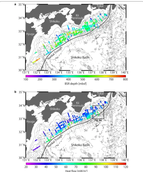
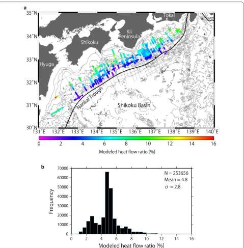
Fig. 3 Distributions of methane hydrate BSRs in the Nankai subduction zone. a Colored dots indicate BSR depths below the seafloor. Survey lines are represented by gray lines. b Colored dots indicate the topographically corrected and uncorrected heat flow derived from the BSRs in this study.
et al. 2012; Li et al. 2014), although intermediate val-ues between hydrostatic and lithostatic pressures were adopted by Ashi et al. (2002). In order to examine the uncertainty caused by these pressure profiles, we cal-culated heat flow values, HFh (Fig. 3b) and HFl
(Addi-tional file 1: Figure S1), from the BSRs using hydrostatic
and lithostatic pressures, respectively, and assessed their differences (HFl− HFh)/HFh× 100 (Fig. 4a). We found
the ratio (HFl− HFh)/HFh× 100 changed by
approxi-mately 4.8% on average (Fig. 4b). The ratio had a consist-ently larger value in shallower areas, while the ratio was smaller in deeper waters, owing to the depth between a
b
the seafloor and the BSR with respect to the thickness of the overlying water column. In addition, convex-upward seafloor regions yielded a large ratio because the water depths were slightly shallower allowing deeper BSRs to develop in this location relative to neighboring areas. The ratio in shallow waters (e.g., at a water depth of 800 m) differed up to approximately 15%.
We also compared the BSR-derived values obtained by assuming hydrostatic and lithostatic pressure regimes to the heat flow HFAPCT3 from an advanced piston corer
temperature tool (APCT3) that penetrated 159 m below the seafloor (mbsf) at Site C0002 of IODP Expedition 315 (Expedition 315 Scientists 2009; Harris et al. 2013) and the heat flow HFprobe from the probe used at the
Kumano Basin near Site C0002 (Hamamoto et al. 2011). The difference (HFh− HFAPCT3)/HFAPCT3× 100 fell within
12%, and the difference (HFl− HFAPCT3)/HFAPCT3× 100
reached approximately 18%. Because the heat flow com-parison may reflect different thermal conductivities, we also calculated the difference using the geothermal gra-dient in the same manner as the heat flow and obtained values of − 1.9 and + 2.9%, assuming hydrostatic and lithostatic pressures, respectively. In contrast, the dif-ference (HFh− HFprobe)/HFprobe× 100 reached
approxi-mately −16%, and the difference (HFl− HFprobe)/
HFprobe× 100 reached approximately − 10%. The
mini-mum difference was the absolute difference between the geothermal gradient value assuming hydrostatic pressure and the APCT3 geothermal gradient. Because the pen-etration depth of the APCT3 was much deeper than that of the probe, differences between the BSR-derived heat
flow and heat flow obtained with the APCT3 were more reliable. Therefore, we constrained the thermal structure using the temperature at the BSRs by assuming hydro-static pressure.
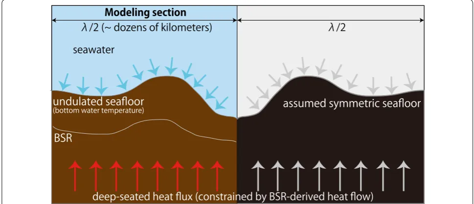
Correction for influence of topography
Surface heat flow values are sensitive to seafloor topog-raphy. This topographic effect was first considered in the Cascadia margin (Ganguly et al. 2000; Hornbach et al. 2012; Phrampus et al. 2017), the Costa Rica margin (Harris et al. 2010), and the Nankai Trough (Harris et al. 2011). Li et al. (2014) suggested that three-dimensional topographic effects should be taken into account to evaluate heat flow variations in the complex topographic region of Cucumber Ridge off Vancouver Island, where the dip angle locally reaches ~ 45°. Variations in heat flow can also be explained by the magnitude and pattern of two-dimensional topographic effects, although the dif-ference between the BSR-derived heat flow and the mod-eled heat flow reached 20 mW/m2 over the steep slope
of Cucumber Ridge (Li et al. 2014). Because our mode-ling sections had gentler slopes falmode-ling within 20° in the dip direction and relatively little topographic variation, within 5° (3° on average) across the modeling sections, our calculation, which considers two-dimensional topo-graphic effects based on Blackwell et al. (1980), was also considered to provide a reasonable model for shallow thermal structures.
The topographic effect was calculated by considering the bottom water temperature and the relief of the sea-floor (Fig. 5). Although topographic effects were also
affected by lithology, the shallow thermal structure in this study was modeled mainly at the prism slope, composed predominantly of mudstone and sandstone (Moore et al. 2001; Strasser et al. 2014); therefore, we ignored the regional lithological variation. In addition, we did not need to consider the influence of seasonal changes in the bottom water temperature on the BSR depth because thermal diffusion from the seafloor to greater depths takes far longer than the seasonal changes (Martin et al. 2004). Therefore, BSR depths could be reliable indices of temperature below the seafloor.
In order to obtain the shallow thermal structure below the seafloor, we solved the following two-dimensional steady-state equation:
where T is the subseafloor temperature, x is the
horizon-tal coordinate, and z is the vertical coordinate. The fol-lowing were employed as boundary conditions: (a) the bottom water temperature at the seafloor from hydro-graphic observation data from the Japan Oceanohydro-graphic Data Center as an upper boundary condition; and (b) a geothermal gradient α at infinitely deep depths in the
absence of a topographic effect. This method modified Blackwell et al.’s (1980) protocol by using temperatures at observed BSR depths to constrain the boundary con-dition (b), as detailed below. We also assumed that the thermal conductivity was uniform and that the heat flow from the deep depths was constant and vertical.
The solution of the heat equation, Eq. (1), constrained by these boundary conditions, was obtained by the fol-lowing series approximation:
where Ak and k are a constant and a wave number, respectively, determined by the boundary conditions. To simplify the calculation, we assumed that the seafloor depth was symmetric from 0 to , where is the
wave-length of Eq. (2). The wavelength was twice as long as
the horizontal distance because we assumed a symmet-ric geometry of the seafloor on the lateral boundaries of the region of interest (Fig. 5). Here, N points of discrete
topographic data with horizontal intervals correspond-ing to the CMP interval were present from 0 to /2, and
we took M (<N−1) points of the series, where M was
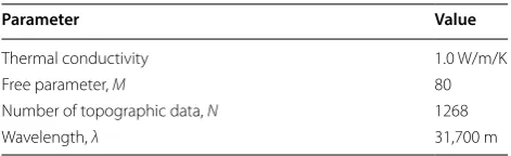
a free parameter. The number of discrete topographic data corresponding to the CMP number varied with each survey line (e.g., N =1268 in the A–B section of Fig. 1). We used a free parameter M of 80 because this value was
smaller than the number from the topographic data of all
(1)
modeling survey lines and an increase in M (e.g., from 80
to 1000 in the A–B section of Fig. 1) had little effect on the thermal structure (0.002 °C on average). The coeffi-cient Ak could be obtained by solving the square matrix of M+1.
We then acquired temperatures at discretized depths using the obtained coefficient, where the vertical inter-val was 3–15 m, depending on the horizontal distance. There were 900 vertical components for each horizontal point. The values obtained using Eq. (2) were referred to as topographically corrected values in this study. The parameter values used for thermal modeling in the A–B section of Fig. 1 are shown in Table 2. The temperatures at the BSR depths were used for the boundary condition (b) to restrict the calculated thermal structure by choos-ing the best coherency between the temperature at the BSRs and the calculated temperature at the same depth of the shallow thermal structure. In particular, the geo-thermal gradient α must be known before the calculation,
and we found the most suitable α in each modeling
sec-tion. The α value was determined so that the calculated
temperature at BSR depths best agreed with the tempera-ture estimated based on the phase boundary. Therefore, we calculated the thermal structure iteratively in order to derive the most suitable geothermal gradient α at
inter-vals of 1 °C/km. The thermal structure was then finalized using the derived geothermal gradient α. We conducted
these procedures in each modeling section; therefore, the geothermal gradient α differed in each modeling section.
The locations of all modeling sections are indicated in Additional file 1: Figures S2 and S3.
Results
Distribution of BSRs
We confirmed the existence of extensive BSRs in the Nan-kai Trough (Fig. 3), ranging from the forearc basins to the prism slope, which was consistent with previous studies (Ashi et al. 2002; Baba and Yamada 2004). BSRs had been thought to be absent from the prism toe off Tokai as well as the trough floor, slope basins, steep slope, and subma-rine canyons. However, this study revealed the develop-ment of acoustic reflectors that parallel the seafloor with seismic reflection profiles that show high-amplitude
Table 2 Parameters used for thermal modeling in the A–B cross section southwest of the Kii Peninsula
The location of the modeling section is indicated in Fig. 1
Parameter Value
Thermal conductivity 1.0 W/m/K
Free parameter, M 80
Number of topographic data, N 1268
reverse-polarity waveforms at the toe and at the trough (trench) floor of the eastern edge of the Nankai subduc-tion margin (Fig. 6), as found in the Costa Rica erosional margin (Pecher et al. 1998). The reflector at the prism toe extended from approximately 1–2 km landward of the trough floor at a water depth of approximately 4000 m. The depth between the seafloor and the reflector was 300–400 mbsf. Similarly, the reflector at the trough floor extended approximately 1 km at a water depth of approx-imately 4000 m. The depth between the seafloor and the reflector was 300–370 mbsf. We interpreted these acous-tic reflectors as BSRs, as further explored in the “ Discus-sion” section.
BSR depths are controlled by in situ temperatures and pressures, and a gas supply to the formation is required for the development of BSRs. Although the trough floor and the prism toe were theoretically deep enough for BSRs to develop, BSRs were generally not observed in these regions, even at great water depths. This suggested a lack of methane in these regions, owing to young hori-zontal trench sediments consisting of alternating per-meable and imperper-meable layers (e.g., Ashi et al. 2002). In addition, picking BSRs that parallel the reflectors of sedimentary layers was technically challenging with low-amplitude reflectors.
The depth between the seafloor and the BSR fluctu-ated between 150 and 800 m in the studied area (Fig. 3a), and uncertainties in the BSR depth were ± 5% consid-ering variation in P-wave velocity, as discussed in the Methods section. A trend of increasing BSR depths from the trough floor to the forearc basin was observed, as reported in previous studies over the prism slope to the forearc basin (Yamano et al. 1982, 1984). Because the BGHS should increase with water depth under a constant heat flow, the observed trend of BSR depth implied that heat flow decreases from the trough floor to the forearc basin. We also observed that the BSR depth was deeper in convex-upward seafloor regions of approximately 120 m and was shallower in convex-downward seafloor regions of approximately 250 m than in neighboring areas (Fig. 7).
Heat flow estimation
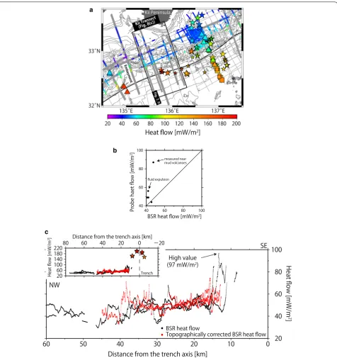
A maximum heat flow from the BSR of 111 ± 14 mW/ m2 was obtained off Shikoku (Fig. 3b), and another high
heat flow of 97 ± 12 mW/m2 was obtained southwest of
Kii Peninsula (Fig. 8c). A minimum of 25 ± 3 mW/m2
was observed off southern Hyuga (Fig. 3b). From off-shore Tokai to Kii Peninsula at a distance of 15–25 km landward of the deformation front, the BSR-derived heat flow of this study ranged from 60 to 80 mW/m2 (Fig. 3b),
and the heat flow from a probe ranged from 60 to 100 mW/m2 (Yamano et al. 2014). At a distance of 40–60 km
landward of the deformation front, the BSR-derived heat flow of this study was 35–50 mW/m2, whereas the data
from the probe measurements indicated heat flow val-ues of 40–60 mW/m2 (Hamamoto et al. 2011). The
dif-ferences between heat flow derived from our BSR and that from the probes used by Yamano et al. (2014) and Hamamoto et al. (2011) fell within the expected dif-ferences between BSR and probe values. We also con-firmed that the differences between the heat flow values from the BSRs and those from the probes in neighbor-ing areas fell within the range of 20%, except for two sites in the Kumano Basin where high heat flow values were observed (Fig. 8b). However, it should be noted that the number of probe measurements near the BSRs (within a distance of approximately 1 km) was limited, especially southwest of Kii Peninsula (Fig. 8a). The high heat flow from probe measurements at the Kumano Basin sites was thought to be affected by fluid expulsion (Hamamoto et al. 2011).
In convex-upward seafloor regions, the BSR was situ-ated at a deeper depth; therefore, the heat flow values there were lower than in neighboring areas (Fig. 7). Rapid sedimentation causes low surface heat flow values, apparently due to a delay in recovery from the disturbed thermal equilibrium. However, sedimentation in the convex-upward seafloor regions was not likely to occur because of their geometry. Therefore, we considered that this low heat flow was caused by topography rather than rapid sedimentation. In contrast, in the convex-down-ward seafloor regions, the BSR was shallower and the values were higher than those in the surrounding areas (Fig. 7), apparently because rapid erosion caused high surface heat flow values. However, erosion in the con-vex-downward seafloor regions was not likely to occur because of their geometry. Therefore, we considered that this high heat flow was caused by topography rather than rapid erosion.
Regional BSR depth variation
a
b
c
Fig. 6 Detected BSRs. a Map of BSR-derived heat flow in the Tokai area. BSRs were detected within the locations marked by the two black circles. Colored dots indicate heat flow values derived from the BSRs. b Seismic reflection image at the prism toe, where BSRs were found, shown with blue
triangles. A P-wave velocity obtained from Site C0002 of the IODP Expeditions (Expedition 314 Scientists 2009) is used for time-to-depth conversion.
c Seismic reflection image at the trough floor, where BSRs were found, shown with blue triangles. A P-wave velocity obtained from Site C0002 of the
of the modeling section A–B (Figs. 1, 8a), and this may have influenced surface heat flow of the A–B section. We evaluated the influence of the embayment on surface heat flow by evaluating only the section orthogonal to the A–B section. The result of this analysis indicated that the embayment (slope of 11° but far away from the modeling sections) influenced surface heat flow of the A–B sec-tion by less than 2%, assuming simplified bathymetry and constant deep-seated heat flux (Fig. 10). Here, we defined the BSR-derived heat flow by taking into account the influence of the undulating seafloor as the cally corrected BSR-derived heat flow. The topographi-cally corrected BSR-derived heat flow was obtained by dividing BSR-derived heat flow by the q/q0 ratio, where q0 and q are, respectively, the heat flow originating from
the deep-seated heat flux and the heat flow estimated at the seafloor from the deep-seated heat flux. After the topographic correction, the BSR-derived heat flow along the Kii Peninsula transect ranged from 30 to 80 mW/m2
at a distance of 10–50 km from the trench axis (Fig. 8c), while the uncorrected BSR-derived heat flow ranged from approximately 30–100 mW/m2. A sudden rise in the
heat flow at a distance of 10–15 km from the trench axis was tempered with the topographic correction.
The estimated BGHS depths and observed BSR depths were expected to agree well. BGHS depths considering the topographic effect (hereafter referred to as “two-dimensional BGHS depths”) were defined as depths at the hydrate-gas phase boundary (Tishchenko et al. 2005) with increasing pressure and modeled temperature from the seafloor, whereas BGHS depths without considering topographic effect (hereafter referred to as “one-dimen-sional BGHS depths”) were depths at the phase boundary (Tishchenko et al. 2005) with linearly increasing pressure
and temperature from the seafloor. As demonstrated in the previous section, BSR-derived heat flow values varied in the regions with a upward or convex-downward seafloor. However, when considering the seafloor topography of the modeling sections, the influ-ence appeared to propagate to only several hundreds of meters in the vertical direction and several kilometers in the horizontal direction. Therefore, the heat flow was predominantly determined by the basal heat flux from the subducting plate. We, therefore, conducted the ther-mal modeling by taking into account the topographic effect based on the heat flux. The two-dimensional BGHS depths calculated from this thermal modeling fit well with the observed BSR depths in both the convex-upward and convex-downward seafloor regions (Fig. 9d). Although the absolute difference between one-dimen-sional BGHS depth and the observed BSR depth reached 180 m at a distance of 11–16 km from the trench axis (Fig. 9d), the absolute difference between the two-dimen-sional BGHS depth and the BSR depth fell within 50 m in this region. Considering the uncertainty in the BSR depth (± 5%), the difference of 50 m was extended to approxi-mately 30–70 m in this region. Similar results could also be found in other investigated profiles (Additional file 1: Figures S4–S23). These results indicated that the topo-graphic effect should be one of the fundamental consid-erations in heat flow estimations and that our thermal modeling accurately expressed the local heat flow at least at depths between the seafloor and the BSR.
As demonstrated in the section discussing the uncer-tainties associated with this study, the total uncertainty in the heat flow from the BSRs was less than 25%. We also conducted an error evaluation of the thermal struc-ture by comparing the maximum (+ 12.5%), average,
Fig. 7 Example of BSR depth variation in convex-upward and convex-downward seafloor regions southwest of Kii Peninsula. BSRs are marked with blue triangles. Their depths are deeper in the convex-upward seafloor region and shallower in the convex-downward seafloor region relative to the neighboring areas. The two-way travel time is converted to subseafloor depth using a P-wave velocity obtained from Site C0002 of the IODP
a
b
c
Fig. 8 BSR-derived heat flows. a Comparison of heat flows from the BSRs, probe measurements, and borehole measurements off the Kii Peninsula.
Colored symbols indicate heat flows measured by probes [squares from Kinoshita et al. (2008), stars from Hamamoto et al. (2011)], boreholes
[trian-gles from Shipboard Scientific Party (1975, 1986a, b), Taira et al. (1991), Moore et al. (2001), Harris et al. (2011), and Marcaillou et al. (2012)], and BSRs
(colored dots from this study). Larger sizes of the square and star symbols reflect better data quality as defined by the authors. Gray lines represent survey lines, and thick lines represent modeled survey lines. The black frame bounds a 60 km wide area encompassing five modeling sections and probe data. b Cross plot showing the topographically uncorrected BSR-derived heat flow and probe heat flow within approximately 1 km of the Kumano Basin. The differences between the heat flows from BSRs and from probes in neighboring areas fall within a range of 20%, except at two
sites, which are thought to be affected by fluid expulsion (Hamamoto et al. 2011). c Heat flow profiles along the transect bounded by the black
frame in (a). The profiles include topographically uncorrected (black dots) and corrected (red dots) BSR-derived heat flows of five modeled seismic lines (gray thick lines within the black frame in (a). Although a sudden rise/drop of the heat flow is observed in the uncorrected data at distances from the trench axis of approximately 15 and 30 km, the change is tempered by topographic correction. The inset figure shows the topographically uncorrected (black dots) and corrected (red dots) BSR-derived heat flows of the five modeled seismic lines and probe heat flows [stars from
a
b
d c
Fig. 9 BSR and BGHS in the convex-upward and convex-downward seafloor regions southwest of the Kii Peninsula. a Bathymetry with the depths
of the observed BSR and the calculated topographically corrected BGHS (2-D) and uncorrected BGHS (1-D). b Plot of q/q0 ratio, where q0 is the heat
flow originating from the deep-seated heat flux, and q is the heat flow estimated at the seafloor from the deep-seated heat flux. A ratio less than
1 indicates that the shallow subseafloor is subject to defocusing induced by the topography, and a ratio larger than 1 indicates that the shallow subseafloor is subject to focusing induced by the topography. c Error evaluation of the thermal modeling by comparison with the temperature of
the BSR (TBSR) using maximum (red line), average (black line), and minimum (blue line) heat flow values. Temperature variations in the BSR fall within
± 3 °C. d Difference in depths between the observed BSR and calculated BGHS values with and without considering the topographic effect. The
and minimum (− 12.5%) basal heat flow (or tempera-ture gradient, α) values (Fig. 9c). The uncertainty yielded
temperature variations on the BSR within ± 3 °C. These temperature variations also yielded variations in two-dimensional BGHS depths falling within ± 70 m.
Discussion
BSRs at the prism toe and trough floor off Tokai
We interpreted acoustic reflectors that parallel the sea-floor with seismic reflection profiles showing high-amplitude reverse-polarity waveforms at the prism toe and at the trough (trench) floor as BSRs. To confirm whether these reflectors originated in methane hydrate, we calculated the theoretical depth of hydrate forma-tion. The available heat flow values near these areas and those acquired at the trough floor with a thermal probe ranged from 80 to 100 mW/m2 (Yamano et al. 2003;
Hamamoto et al. 2011). Assuming a thermal conductivity of 1.0 W/m/K, the one-dimensional BGHS depths were calculated to be 220–270 mbsf, while the observed BSR depth was 300–400 mbsf. Considering the absence of sur-face heat flow and P-wave velocity in the sediment very close to these areas (within distances of approximately 1 km) where BSRs were found, these reflectors could be interpreted to be methane hydrate BSRs. Artificial noises paralleling the seafloor, such as a waveform induced by airgun bubbles, were not observed throughout the region. Multiple reflectors could also be dismissed because of the discrepancy between the two depths.
Heat flow variation
The heat flow was highly variable at a distance from the trench axis along the Kii Transect (Fig. 8c). The high BSR-derived heat flow value of 97 ± 12 mW/m2 was locally
obtained along the lower landward slope in the south-western region offshore of the Kii Peninsula, where the relatively young plate (Mahony et al. 2011) was subduct-ing. This region is located in a convex-downward seafloor and is subject to the focusing effect induced by topogra-phy. The high heat flow value was estimated to be 61 ± 8 mW/m2 after topographic correction. The difference
between the topographically uncorrected and corrected values was 36 ± 20 mW/m2 (Fig. 8c). This corrected heat
flow value was not anomalously high compared with the surrounding areas. Therefore, the topographic effect was a primary contributor to the very small-scale variation in heat flow in this region.
The minimum BSR-derived heat flow of 25 ± 3 mW/ m2 was obtained off southern Hyuga, where the oceanic
plate was deeply subducting in the Nankai margin. This region is located in a convex-upward seafloor and is sub-ject to the defocusing effects induced by topography. The minimum value of corrected heat flow was 29 ± 4 mW/
m2. The slab deepening and the topography were likely
to cause the minimum heat flow value in our study area. Although the sedimentation effect appeared to cause the lower heat flow (Hutchison 1985; Wang et al. 1993), according to our seismic profile, this region of low heat flow corresponded to ridge topography rather than a sed-imentary basin.
Possible causes of BSR depth anomalies other than topography
As mentioned in the previous section, the topographic effect was expected to be a primary contributor to the variation in heat flow values in convex-upward and convex-downward seafloor regions (Fig. 8c). After topo-graphic correction, there were some sudden increases in BSR-derived heat flows throughout the modeling tion, even far away from the lateral boundaries of the sec-tion (Fig. 8c, Additional file 1: Figure S24). These sudden increases may have reflected advective fluid flow where a thrust fault intersects the seafloor, although this fault cannot be confirmed from our seismic profiles. In order to obtain evidence for advective fluid flow, submersible exploration would be required. Therefore, the possibility of advection could not be excluded. Although recent ero-sion also causes sudden increases in heat flow, we could not confirm erosion from bathymetry features either. Moreover, sudden increases may be due to recent uplift, where thermal equilibrium had not yet been reached. Therefore, we may have actually overestimated heat flow values at some uplifted areas via topographic correc-tion (e.g., at a distance of approximately 15 km from the trench axis in Additional file 1: Figure S14). More surveys that include measurements from probes and boreholes were needed to identify these phenomena.
The differences in BSR depths between our model and observations were large in some places. Although P-wave velocities that were different from the true velocity was one factor generating the differences, the influence was small because the BSR depths below the seafloor were shallow. For example, the error associated with BSR depths was 20 m assuming a P-wave velocity error of 100 m/s and a two-way travel time between the seafloor and the BSR of 0.4 s. We calculated the two-dimensional BGHS depths considering the 25% uncertainty demon-strated in the “Uncertainty in BSR-derived heat flow” sec-tion. In particular, we recalculated the thermal structure using the maximum (+ 12.5%) and minimum (− 12.5%) heat flows (geothermal gradient, α) and calculated the
most of the differences fell within 40 m (approximately one standard deviation of the differences between two-dimensional BGHS and BSR).
The differences that could not be explained by two-dimensional topographic effects, considering the uncer-tainty of BSR-derived heat flow, may have been due to prominent sedimentation and erosion. Sedimentation and erosion could be identified from the combination of geometries and positive and negative differences between the two-dimensional BGHS and BSR, although fluid flow, salinity variations, higher-order hydrocarbons, and three-dimensional topography could also explain the dif-ferences. If the calculated two-dimensional BGHS depths were shallower than the observed BSR depths, then the area was suggested to have suffered from the cooling effect of sedimentation. Likewise, calculated two-dimen-sional BGHS depths that were deeper than the observed depths suggested that the area suffered from erosion.
Sea level change also alters the depths of BSRs by inducing pressure changes in the water column (e.g., Kre-mer et al. 2017). However, a sea level change of 100 m
produces only a 3.7% variation in heat flow at a water depth of 1500 m, assuming a uniform geothermal gradi-ent of 40 °C/km (Expedition 315 Scigradi-entists 2009), if the BSR depths have not yet reached thermal equilibrium after the sea level change. Because the effect decreases with water depth and most of the modeling area was deeper than 1500 m, sea level change was negligible for estimations of sedimentation and erosion.
Validity and significance of our thermal modeling
We examined the differences between the two-dimen-sional BGHS depths and the observed BSR depths of all modeled sections in order to confirm whether the thermal modeling accurately expressed the subseafloor temperatures (Fig. 11). The differences between the two-dimensional BGHS depths from our thermal struc-ture and the observed BSR depths ranged from − 110 to + 140 m (Fig. 11b), whereas, the differences in the one-dimensional BGHS depths (i.e., BGHS depths without considering the topographic effect) ranged from − 290 to + 200 m (Fig. 11a). This indicated that our modeled a
b
thermal structure that considers the topographic effect was more consistent with the subseafloor temperature estimated from the observed BSR depths.
Frictional heating along a subducting plate interface and radioactive heat production could change the ther-mal structure, even though the effective coefficient of friction was thought to be low in the Nankai Trough area (Yoshioka and Murakami 2007; Hamamoto et al. 2011; Ji et al. 2016). Most subduction zone thermal models do not consider topography with a wavelength of a few kilo-meters or less, as was treated by this study. In that case, the results of such a thermal model should be compared with heat flow observations that have been corrected for the small wavelength topography. The frictional heating and radioactive heat production could be estimated more precisely using a wide range of heat flow values in con-junction with our result for the shallow thermal struc-ture because the topographic correction changed up to 36 mW/m2 of the BSR-derived heat flow in this study
(Fig. 8c).
The time required to reach thermal equilibrium within subseafloor sequences through thermal diffusion is thought to be affected by the methane hydrate fraction and the latent heat of hydrate formation or dissociation (Kinoshita et al. 2011). Therefore, the sedimentation and erosion that occur within thermal equilibrium can be estimated by assuming the total hydrate fraction and an initial disturbance, such as rapid sedimentation or
erosion. Although sedimentation and erosion can be estimated from anomalies in the local heat flow, erosion in convex-upward seafloor regions or sedimentation in convex-downward seafloor regions apparently mitigate local heat flow anomalies. In these areas, it is difficult to discern each phenomenon through only BSR depth data. However, comparing two-dimensional BGHS depths by considering the topographic effect in conjunction with the observed BSR depths can aid investigations of these phenomena. In summary, the shallow thermal structure that considers the topographic effect is of use in estimat-ing the subseafloor temperature and also for understand-ing past surface geological phenomena, such as active sedimentation or erosion.
Conclusions
We investigated the distributions of bottom-simulating reflectors (BSRs) in the landward region of the Nankai subduction zone. We also estimated heat flow from BSR depths, evaluated the error, and modeled the shallow thermal structure constrained by the temperature at BSR depths. The main results are summarized as follows.
1. BSRs were present across the area, ranging from the forearc basin to the accretionary prism slope. These were verified for the first time at the accretionary prism toe and at the trough floor offshore of the Tokai region.
a b
Fig. 11 Differences between the BGHS and BSR depths, compiled from 21 seismic profiles (24,329 points). a Differences between the
one-dimen-sional BGHS depths without considering the topographic effect and the BSR depths. The differences range from − 290 to + 200 m. The mean value
and the standard deviation are 0 and 63 m, respectively. b Differences between the two-dimensional BGHS depths considering the topographic
2. BSR depths below the seafloor were larger in con-vex-upward seafloor regions and smaller in convex-downward seafloor regions than in neighboring areas. These regional variations could be explained by the defocusing and focusing effects induced by the topography. In addition, our model helps detect past surface geological phenomena, such as prominent sedimentation or erosion.
3. The total uncertainty of the BSR-derived heat flow should fall within 25%, considering allowable changes in the P-wave velocity in seawater and sediment, the geothermal gradient, and thermal resistance.
Abbreviations
BSRs: bottom-simulating reflectors; BGHS: base of gas hydrate stability; MCS: multi-channel seismic; PHP: Philippine Sea plate; CMP: common mid-point; IODP: Integrated Ocean Drilling Program; ODP: Ocean Drilling Program; APCT3: advanced piston corer temperature tool.
Authors’ contributions
AO calculated BSR-derived heat flow and thermal structure, and drafted the manuscript. HO interpreted seismic reflection profiles. AK drafted the sub-routine code for calculation of BSR-derived heat flow. JA designed the study with AO. All authors contributed to the scientific discussions and manuscript inputs. All authors read and approved the final manuscript.
Author details
1 Atmosphere and Ocean Research Institute, The University of Tokyo, 5-1-5
Kashiwanoha, Kashiwa, Chiba 277-8564, Japan. 2 Graduate School of
Fron-tier Sciences, The University of Tokyo, 5-1-5 Kashiwanoha, Kashiwa, Chiba 277-8564, Japan. 3 Earthquake Research Institute, The University of Tokyo,
1-1-1, Yayoi, Bunkyo-ku, Tokyo 113-0032, Japan. 4 Institut für Geologie,
Univer-sität Innsbruck, Innrain 52f, 6020 Innsbruck, Austria.
Acknowledgements
We are grateful to Y. Kawada for the original code for thermal modeling, J.-O. Park, crew, and scientific parties of R/V Kairei, Kaiyo, and Polar Princess for acquiring MCS data used in this study. We are also grateful to R. Harris for his fruitful comments on an early version of the manuscript. We thank anony-mous reviewers for helpful comments. AK is currently funded by the Austrian Science Fund (FWF-P29678). Generic Mapping Tools (GMT) software (Wessel and Smith 1998) is used to draft some figures.
Competing interests
The authors declare that they have no competing interests.
Availability of data and materials
MCS reflection data conducted by R/V Kairei and Kaiyo can be obtained from Crustal Structural Database Site (https://www.jamstec.go.jp/jamstec-e/ IFREE_center/index-e.html). Hydrographic observation data of bottom water temperature can be obtained freely from the Japan Oceanographic Data Center (http://www.jodc.go.jp/jodcweb/index_j.html). Other data presented in Results section of this study are available upon request by emailing the corresponding author.
Ethics approval and consent to participate Not applicable.
Additional file
Additional file 1. Supporting Information regarding the location map of thermal modeling, heat flow profiles, and BSR-derived heat flow assuming lithostatic pressure. Thermal structure and BSR-derived heat flow in the Nankai subduction margin.
Funding
This work was partially supported by JSPS KAKENHI Grant Number 15H02988.
Publisher’s Note
Springer Nature remains neutral with regard to jurisdictional claims in pub-lished maps and institutional affiliations.
Received: 25 September 2017 Accepted: 5 April 2018
References
Aoki Y, Tamano T, Kato S (1982) Detailed structure of the Nankai trough from migrated seismic sections: studies in continental margin geology. AAPG Mem 34:309–322
Ashi J, Tokuyama H, Taira H (2002) Distribution of methane hydrate BSRs and its implication for the prism growth in the Nankai Trough. Mar Geol 187:177–191. https://doi.org/10.1016/S0025-3227(02)00265-7
Baba K, Yamada Y (2004) BSRs and associated reflections as an indicator of gas hydrate and free gas accumulation: an example of accretionary prism and forearc basin system along the Nankai Trough, off Central Japan. Resour Geol. 54:11–24. https://doi.org/10.1111/j.1751-3928.2004. tb00183.x
Bangs NL, Sawyer DS, Golovchenko X (1993) Free gas at the base of the gas hydrate zone in the vicinity of the Chile triple junction. Geology 21:905–908
Blackwell DD, Steele JL, Brott CA (1980) The terrain effect on terrestrial heat flow. J Geophy Res Solid Earth 85:4757–4772. https://doi.org/10.1029/ JB085iB09p04757
Chen L, Chi WC, Wu SK, Liu CS, Shyu CT, Wang Y, Lu CY (2014) Two-dimensional fluid flow models at two gas hydrate sites offshore south-western Taiwan. J Asian Earth Sci 92:245–253
Chhun C, Kioka A, Jia J, Tsuji T (2017) Characterization of hydrate and gas reser-voirs in plate convergent margin by applying rock physics to high-reso-lution seismic velocity model. Mar Petrol Geol. https://doi.org/10.1016/j. marpetgeo.2017.12.002
Claypool GE, Kaplan IR (1974) The origin and distribution of methane in marine sediments. Nat Gases Mar Sediment Mar Sci 3:99–139
Cook AE, Anderson IB, Malinverno A, Mrozewski S, Goldberg SD (2010) Electri-cal anisotropy due to gas hydrate-filled fractures. Geophysics 75(6):F173– F185. https://doi.org/10.1190/1.3506530
Davis EE, Wang K, Becker K, Thomson RE, Yashayaev I (2003) Deep-ocean temperature variations and implications for errors in seafloor heat flow determinations. J Geophys Res. https://doi.org/10.1029/2001jb001695
Dickens GR, Quinby-Hunt MS (1994) Methane hydrate stability in seawater. Geophys Res Lett 21(19):2115–2118
Expedition 314 Scientists (2009) Expedition 314 Site C0002. In: Kinoshita M, Tobin H, Ashi J, Kimura G, Lallemant S, Screaton EJ, Curewitz D, Masago H, Moe KT, Expedition 314/315/316 Scientists (ed) Proceedings of the Inte-grated Ocean Drilling Program, 314/315/316. Washington, DC, pp 1–77 Expedition 315 Scientists (2009) Expedition 315 Site C0002. In: Kinoshita M,
Tobin H, Ashi J, Kimura G, Lallemant S, Screaton EJ, Curewitz D, Masago H, Moe KT, Expedition 314/315/316 Scientists (ed) Proceedings of the Inte-grated Ocean Drilling Program, 314/315/316. Washington DC, pp 1–75 Feistel R (2008) A Gibbs function for seawater thermodynamics for −6 to 80°C
and salinity up to 120 g kg−1. Deep Sea Res I 55:1639–1671
Foucher JP, Nouzé H, Henry P (2002) Observation of a double BSR on the Nakai slope. Mar Geol 187:161–175
Ganguly N, Spence GD, Chapman NR, Hyndman RD (2000) Heat flow varia-tions from bottom simulating reflectors on the Cascadia margin. Mar Geol 164:53–68
Grevemeyer L, Villinger H (2001) Gas hydrate stability and the assessment of heat flow through continental margins. Geophys J Int 145:647–660 Hamamoto H, Yamano M, Goto S (2005) Heat flow measurement in shallow
seas through long-term temperature monitoring. Geophys Res Lett 32:L21311. https://doi.org/10.1029/2005gl024138
off the Kii Peninsula. Geochem Geophys Geosys 12:Q0AD20. https://doi. org/10.1029/2011gc003623
Harris RN, Grevemeyer I, Ranero CR, Villinger H, Barckhausen U, Henke T, Mueller C, Neben S (2010) Thermal regime of the Costa Rican convergent margin: 1. Along-strike variations in heat flow from probe measurements and estimated from bottom-simulating reflectors. Geochem Geophys Geosyst 11:Q12S28. https://doi.org/10.1029/2010gc003272
Harris RN, Schmidt-Schierhorn F, Spinelli G (2011) Heat flow along the NanT-roSEIZE transect: results from IODP Expeditions 315 and 316 offshore the Kii Peninsula. Japan. Geochem Geophys Geosyst 12:Q0AD16. https://doi. org/10.1029/2011gc003593
Harris R, Yamano M, Kinoshita M, Spinelli G, Hamamoto H, Ashi J (2013) A synthesis of heat flow determinations and thermal modeling along the Nankai Trough, Japan. J Geophys Res 118:2687–2702. https://doi. org/10.1002/jgrb.50230
Harris RN, Spinelli GA, Fisher AT (2017) Hydrothermal circulation and the ther-mal structure of shallow subduction zones. Geosphere 13(5):1425–1444 Henrys SA, Ellis S, Uruski C (2003) Conductive heat flow variations from
bottom-simulating reflectors on the Hikurangi margin, New Zealand. Geophys Res Lett 30:1065
Hornbach MJ, Bangs NL, Berndt C (2012) Detecting hydrate and fluid flow from bottom simulating reflector depth anomalies. Geology 40(3):227–230
Hutchison I (1985) The effects of sedimentation and compaction on oceanic heat flow. Geophys J R Astron Soc 82:439–459. https://doi.org/10.1111/ j.1365-246X.1985.tb05145.x
Hyndman RD, Wang K (1993) Thermal constraints on the zone of major thrust earthquake failure: the Cascadia subduction zone. J Geophys Res B98:2039–2060. https://doi.org/10.1029/92JB02279
Ji Y, Yoshioka S, Matsumoto T (2016) Three-dimensional numerical modeling of temperature and mantle flow fields associated with subduction of the Philippine Sea plate, southwest Japan. J Geophys Res Solid Earth 121:4458–4482. https://doi.org/10.1002/2016JB012912
Kanamori H (1972) Tectonic implications of the 1944 Tonankai and the 1946 Nankaido earthquakes. Phys Earth Planet Inter 5:129–139
Kinoshita M, Kanamatsu T, Kawamura K, Shibata T, Hamamoto H, Fujino K (2008) Heat flow distribution on the floor of Nankai Trough off Kumano and implications for the geothermal regime of subducting sediments. JAMSTEC Rep Res Dev 8:13–28
Kinoshita M, Tobin H, Ashi J, Kimura G, Lallemant S, Screaton EJ, Curewitz D, Masago H, Moe KT, Expedition 314/315/316 Scientists (2009) NanTroSEIZE stage 1: investigations of seismogenesis, Nankai Trough, Japan. In: Proceedings IODP/315/316. https://doi.org/10.2204/iodp. proc.314315316.123
Kinoshita M, Moore GF, Kido YN (2011) Heat flow estimated from BSR and IODP borehole data: implication of recent uplift and erosion of the imbricate thrust zone in the Nankai Trough off Kumano. Geochem Geophys Geo-syst 12:Q0AD18. https://doi.org/10.1029/2011gc003609
Kremer K, Usman MO, Satoguchi Y, Nagahashi Y, Vadakkepuliyambatta S, Pani-eri G, Strasser M (2017) Possible climate preconditioning on submarine landslides along a convergent margin, Nankai Trough (NE Pacific). Prog Earth Planet Sci 4:20. https://doi.org/10.1186/s40645-017-0134-9
Kvenvolden KA (1988) Methane hydrate—a major reservoir of car-bon in the shallow geosphere? Chem Geol 71:41–51. https://doi. org/10.1016/0009-2541(88)90104-0
Kvenvolden KA, McDonald TJ (1985) Gas hydrates of the Middle America Trench—Deep Sea Drilling Project Leg 84. In: Von Huene R, Aubouin J et al (eds) Initial Reports DSDP 84. US Govt Printing Office, Washington, pp 667–682. https://doi.org/10.2973/dsdp.proc.84.123.1985
Li HL, He T, Spence GD (2014) North Cascadia heat flux and fluid flow from gas hydrates: modeling 3-D topographic effects. J Geophys Res 119:99–115.
https://doi.org/10.1002/2013JB010101
Mahony SH, Wallace LM, Miyoshi M, Villamor P, Sparks RSJ, Hasenaka T (2011) Volcano-tectonic interactions during rapid plate-boundary evolution in the Kyushu region SW Japan. Geol Soc Am Bull 123:2201–2223 Marcaillou B, Spence G, Collot J-Y, Wang K (2006) Thermal regime from bottom
simulating reflectors along the north Ecuador–south Colombia margin: relation to margin segmentation and great subduction earthquakes. J Geophys Res 111:B12407. https://doi.org/10.1029/2005JB004239
Marcaillou B, Henry P, Kinoshita M, Kanamatsu T, Screaton E, Daigle H, Harcouët-Menou V, Lee Y, Matsubayashi O, Kyaw Thu M, Kodaira S,
Yamano M, Expedition IODP, 333 Scientific Party (2012) Seismogenic zone temperatures and heat-flow anomalies in the To-nankai margin segment based on temperature data from IODP Expedition 333 and thermal model. Earth Planet Sci Lett 349–350:171–185. https://doi.org/10.1016/j. epsl.2012.06.048
Markl RG, Bryan GM, Ewing JI (1970) Structure of the Blake-Bahama Outer Ridge. J Geophys Res 75:4539–4555. https://doi.org/10.1029/ JC075i024p04539
Martin V, Henry P, Nouzé H, Noble M, Ashi J, Pascal G (2004) Erosion and sedimentation as processes controlling the BSR-derived heat flow on the Eastern Nankai margin. Earth Planet Sci Lett 222:131–144. https://doi. org/10.1016/j.epsl.2004.02.020
Miller JJ, Lee MW, von Huene R (1991) An analysis of a seismic reflection from the base of a gas hydrate zone, offshore Peru. Am Assoc Pet Geol B 75:910–924
Moore GF, Taira A, Klaus A, Party SS (2001) Proceedings of the Ocean Drilling Program. Initial Reports, vol 190. Ocean Driling. Program. College Station, TX. https://doi.org/10.2973/odp.proc.ir.190.2001
Morita S, Ashi J, Aoike K, Kuramoto S (2004) Evolution of Kumano basin and sources of clastic ejecta and pore fluid in Kumano mud volcanoes, Eastern Nanaki Trough. In: Proceedings of the international symposium on methane hydrates and fluid flow in upper accretionary prisms. Engineering Geology Laboratory, Department of Civil & Earth Resources Engineering, Kyoto University, Kyoto, pp 92–99
Otsuka H, Morita S, Tanahashi M, Ashi J (2015) Foldback reflectors near meth-ane hydrate bottom-simulating reflectors: indicators of gas distribution from 3D seismic images in the eastern Nankai Trough. Isl Arc 24(2):145– 158. https://doi.org/10.1111/iar.12099
Pecher IA, Ranero CR, von Huene R, Minshull TA, Singh SC (1998) The nature and distribution of bottom simulating reflectors at the Costa Rican convergent margin. Geophys J Int 133:219–229. https://doi. org/10.1046/j.1365-246X.1998.00472.x
Phrampus BJ, Harris RN, Tréhu AM (2017) Heat flow bounds over the Cascadia margin derived from bottom simulating reflectors and implica-tions for thermal models of subduction. Geochem Geophys Geosys 18(9):3309–3326
Satake K (2015) Geological and historical evidence of irregular recurrent earthquakes in Japan. Philos Trans R Soc A. https://doi.org/10.1098/ rsta.2014.0375
Seno T, Stein S, Gripp AE (1993) A model for the motion of the Philippine Sea plate consistent with NUVEL-1 and geological data. J Geophys Res 98:17941–17948
Shipboard Scientific Party (1975) Site 298, Initial Reports, Deep Sea Drilling Pro-ject, vol 31, pp 317–350. https://doi.org/10.2973/dsdp.proc.31.109.1975
Shipboard Scientific Party (1986a) Site 582, Initial Reports, Deep Sea Drilling Project, vol 87, pp 35–122. https://doi.org/10.2973/dsdp.proc.87.103.1986
Shipboard Scientific Party (1986b) Site 583, Initial Reports, Deep Sea Drilling Project, vol 87, pp 123–256. https://doi.org/10.2973/dsdp. proc.87.104.1986
Shipley TH, Houston MH, Buffler RT, Shaub FJ, McMillen KJ, Ladd JW, Worzel JL (1979) Seismic reflection evidence for the widespread occurrence of possible gas-hydrate horizons on continental slopes and rises. Am Assoc Pet Geol B 63:2204–2213
Spinelli GA, Wang K (2008) Effects of fluid circulation in subducting crust on Nankai margin seismogenic zone temperatures. Geology 36:887–890.
https://doi.org/10.1130/G25145A
Stein CA, Stein S (1992) A model for the global variation in oceanic depth and heat flow with lithospheric age. Nature 359:123–129
Stoll RD, Ewing JI, Bryan GM (1971) Anomalous wave velocities in sediments containing gas hydrates. J Geophys Res 76:2090–2094
Strasser M, Dugan B, Kanagawa K, Moore GF, Toczko S, Maeda L, the Expedition 338 Scientist (2014) Site C0002. In: Proceedings of Integrated Ocean Drill-ing Program, vol 338. https://doi.org/10.2204/iodp.proc.338.103.2014
Taira A, Hill I, Firth J, Shipboard Scientific Party (1991) Proceedings of the Ocean Drilling Program. Initial Reports 131. Ocean Drilling Program, Col-lege Station, TX. https://doi.org/10.2973/odp.proc.ir.131.107.1991
Tishchenko P, Hensen C, Wallmann K, Wong CS (2005) Calculation of the stabil-ity and solubilstabil-ity of methane hydrate in seawater. Chem Geol 219:37–52 Tobin H, Hirose H, Saffer D, Toczko S, Maeda L, Kubo Y, the Expedition 348
Townend J (1997) Estimates of conductive heat flow through bottom-simu-lating reflectors on the Hikurangi and southwest Fiordland continental margins, New Zealand. Mar Geol 141:209–220
Wagner W, Pruß A (2002) The IAPWS formulation 1995 for the thermodynamic properties of ordinary water substance for general and scientific use. J Phys Chem Ref Data 31:387–535. https://doi.org/10.1063/1.1461829
Wang K, Hyndman RD, Davis EE (1993) Thermal effects of sediment thickening and fluid expulsion in accretionary prisms: model and parameter analysis. J Geophys Res 98(B6):9975–9984. https://doi.org/10.1029/93JB00506
Wang K, Hyndman RD, Yamano M (1995) Thermal regime of the Southwest Japan subduction zone: effects of age history of the subducting plate. Tectonophysics 248:53–69
Wessel P, Smith WHF (1998) New, improved version of Generic Mapping Tools released. EOS Trans Am Geophys Union 79:579
Yamano M, Uyeda S, Aoki Y, Shipley TH (1982) Estimates of heat flow derived from gas hydrates. Geology 10:339–343. https://doi. org/10.1130/0091-7613(1982)10<339:eohfdf>2.0.co;2
Yamano M, Honda S, Uyeda S (1984) Nankai trough: a hot trench? Mar Geo-phys Res 6:187–203. https://doi.org/10.1007/BF00285959
Yamano M, Kinoshita M, Goto S, Matsubayashi O (2003) Extremely high heat flow anomaly in the middle part of the Nankai Trough. Phys Chem Earth 28:487–497
Yamano M, Kawada Y, Hamamoto H (2014) Heat flow survey in the vicinity of the branches of the megasplay fault in the Nankai accretionary prism. Earth Planets Space 66(1):126. https://doi.org/10.1186/1880-5981-66-126
Yoshioka S, Murakami K (2007) Temperature distribution of the upper surface of the subducted Philippine Sea plate along the Nankai Trough, south-west Japan, from a three dimensional subduction model: relation to large interplate and low-frequency earthquakes. Geophys J Int 171:302–315.