Wavelet Network Modeling Method Based on Radiation
Characteristics of Array Antenna
Qi LI
*and Zhi-guo ZHANG
University of Electronic Science and Technology of China, Chengdu, 611731, China *Corresponding author
Keywords: Wavelet network, Frequency band characteristics, Array antenna radiation field, Online modeling.
Abstract. In complex electromagnetic environment, the training data contains a lot of noise, which can make classic neural networks overfit easily. In order to solve this problem, a new method based on sampling theory is proposed for constructing models. Through analyzing wavelet networks and radiation fields in the frequency domain, it is proved that the new method can effectively reduce noise on models and help wavelet networks obtain a good generalization. In the simulation, the new method is compared with regularization techniques. The results show that the new method can prevent networks from overfitting and is more robust to noise.
Introduction
Radiation models are essential in testing and diagnosing antenna performances. For now, there are two methods to build an antenna radiation model: one is a classical physics method; the other is using neural network.
The former method, generally, is based on the electromagnetic theory and can obtain a high accurate model[1][2].However, this method is to great depends on the solutions of electromagnetic equations such as Maxwell equations, and it is still a worldwide problem on obtain the solution of Maxwell equations under complex boundary conditions.
The latter method always construct models by the characteristics of training data, so that it can avoid solving the complex equations in former method[3][4]. However, in complex environment, the training data always contain a lot of noise and it will lead the network to overfitting.
In order to find a way to solve the problems above, we analyze the frequency band of wavelet network and antenna radiation models, get the result that both of them have a limited frequency band, based on which a modeling method has been proposed. Simultaneously, the filtering algorithm based on sampling theory is applied in this wavelet network, to prevent the interference of the noise. Theoretical analysis proves the feasibility and effectiveness of this method. In the simulation, we compare this method with RBF network, the results show that the proposed method can reduce the influence of noise more effectively.
Frequency Band Characteristics of Wavelet Network
Wavelet network is a topological expansion of wavelet series. There are many kinds of structures of wavelet network, the structure proposed by literature [5] will be used in this paper, which is shown in Figure 1.
The Figure 1has a mathematical expression
( ) (2J )
ne k
k
f x
c xk(1) where{ }ck is the output weights, 2Jis the input weights, ( )
x
is the scaling function, and kis the
Figure 1. The structure of wavelet network.
The ( )x is highly concentrated in time and frequency domains, so we can get the same result of
the fne( )x . More importantly, in the frequency domain, the fne( )x satisfies the following expression
2
2 2 2
, 2
ˆ ˆ
| ( ) | J w| ( ) | 2 | |
J w
b J
ne b ne k J k
f w dw f w dw c
(2)[6]there, fˆ ( )ne w is the Fourier transform of fne( )x , bw is a constant, while is a positive real number that small enough. Inequality (2) means that the frequency band of the wavelet network
( ) ne
f x can be approximated in
[ 2J , 2J ] w w
b b
(3)
in formula (3), the bw is a constant, and the 2
Jis the input weights, so that the frequency band of
( )
ne
f x is limited and only related to the input weight 2J.
Frequency Band Characteristics of Antenna Radiation Model Frequency Band Analysis of Linear Array Antenna
For a linear array antenna of N radiation units that distribute randomly, their total electric field
in the far field can be expressed as
( , ) 1
( , ) N i
i i
E
I e (4) [7]where Ii is the complex current of the ith radiation unit, and are the pitch angle and the azimuth angle of the antenna, while e i( , )
is the phase of the ith radiation unit that with respect to the reference point.
Since in the far field, the electric field has nothing to do with the azimuth angle , and assume that all the units have the same separation d. so the formula (4) has another expression
( 1)( sin ) 1
(sin ) N j n kd n n
E I e
(5)where
2 /
k (6)
and is the wavelength.
Normally, all the radiation units have the same complex current, i.e. InI0, so we have
( 1)( sin ) sin ( 1)( sin )
0 1 0
(sin ) N j n kd (1 jkd ... j N kd )
n
E I
e I e e (7)0
(sin )
1 (cos sin ) (sin sin )
E I
kd j kd
(8)
And, we all know that
| (sin ) |E E(sin ) (sin ) E (9)
insert the equation (8) into the equation (9), and simplify it
0
sin(( sin ) / 2)
| (sin ) |
sin(( sin ) / 2) Nkd E I kd (10) For the [ , ], so that
sin [ 1,1] (11) According to the theory of antenna design, the equivalent aperture of the antenna should be equal to or greater than a quarter of the electromagnetic wavelength[8]. In order to put as many units as possible on the plane, we consider the equivalent aperture d/ 4. And put it in the equation (6),
we can get
2
kd
(12) For simplicity, let xsin, so the equation (10) can be expressed as
0
sin( / 4)
| (sin ) | | ( ) |
sin( / 4)
N x
E E x I
x (13) From formula (11), on the other hand, we havex/ 4 [ / 4, / 4] , which meet the approximation of sinxx, so we can let
sin(x/ 4)x/ 4 (14)
So that the equation (13) can be expressed as
0 0
sin( / 4) sin( / 4)
| ( ) | | ( ) |
/ 4 / 4
N x N x
E x E x I NI
x N x
(15) where ( ) 0 sin( / 4)
/ 4
N x
E x I
N x
,x [ 1,1], and the Fourier transform of E x( ) is
1 0 1
sin( / 4) ( ) ( )
/ 4
iwx N x iwx
F w E x e dx I e dx
N x
(16)For simplicity, let tNx/ 4, and get
4 0 4 sin( ) ( ) N iwt N t
F w I e dt
t
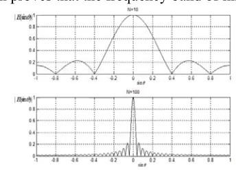
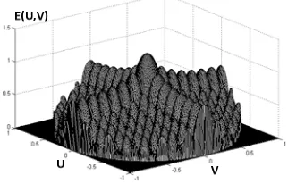
(17) From the equation (17), we find that the E x( ) can be approximated as a Shannon function withthe independent variableof xsin( ) .
To validate the conclusions above, we get the pictures of the equation (15) and (17) with N10
and N 100, which is shown in Figure 2 and 3 separately. The two pictures show the characteristics
which proves that the frequency band of linear array antenna is limited.
[image:4.612.102.274.77.204.2] [image:4.612.327.500.80.199.2]w w
Figure 2. The characteristics in time domain. Figure 3. The characteristics in frequency domain.
Convergence Algorithm Based On Sampling Theory
From the analysis above, we can find that both wavelet networks and the radiation field of array antenna are band limited, which inspires us to use the wavelet network to overcome the interference of the noise when modeling. However, the traditional algorithm rarely notice the influence of the noise, which always result the networks in overfitting.
In order to solve this problem, we decide to use the algorithm that proposed in the document[6]. This algorithm is based on sampling theories and makes full use of the frequency characteristics of wavelet network. it is proved that this algorithm has good convergence and filtering properties, which can effectively reduce the effects of noise and prevent networks from overfitting.
In this algorithm, the training data need to satisfy the sampling theory, while for the wavelet network, the input weights can be expressed as
2J
s w
T b
(19)
the threshold k is
2J 2J
mN k n (20)
And for output weights, it can be solved by the gradient descent iterative course:
( 1) ( 1)
( 1) ( ) ( )
k k
s m n
k k k
f
e F C
C C A e
(21)
in the equation(19), bw is a constant that only related to the scaling function, Ts is the sampling period. In the inequality (20), interval [0,N] is the support of the scaling function, and the interval
[ , ]m n is the training interval that need to be covered. And in the equation (21), the column vector
( )k
e is the error of interpolation by the wavelet network at kth step, the column vector C( )k
is the output weight at kth step, [ ( )... (1 )]
T
s s s m
F f x f x , where x1...xnare the input training data[6].
The Structure and Parameters of Wavelet Network Training Sample Selection Conditions
From the algorithm, we know that the training data need to satisfy the sampling theory, that is to say, the sampling frequency fs need to satisfy the inequality 2
s m
f f , where fm is the maximum frequency of equation (19) in each direction, which means that fmN/ 4. So, we can get that
2 / 2
s m
s
f N (22)
since the higher the sampling frequency, the higher the accuracy of the model, so in many cases, fs is generally greater than N/ 2.
Training Steps of Wavelet Network
According to the descriptions of previous sections, the training process of wavelet network can be concluded as following steps:
1) First, get the sampling period Ts from the equation (22), and collect the training data that satisfy the period Ts.
2) Second, choose a appropriate scaling function ( )x , and get the constant bw it. Put the bw
and Ts into the equation (19) to get the input weight 2 J.
3) Third, use a set of random numbers to initialize the output weight cJ k, . 4) Then, update the output weight cJ k, by using the gradient descent iterative.
Experiment and Simulation Object of Simulation
The simulation object is a rectangle array antenna that construct in the laboratory, for we only to verify the feasibility of the method, we don’t care its other capabilities(for example, it has a poor directivity). In our simulation, we choose the array units Nx Ny N15, the signal frequency is
600MHZ, so the antenna apertured0.125m, and the sampling period Ts 2 / 15.
[image:5.612.228.389.415.518.2]The data is collected 10 meters away from the antenna in order to keep in the far field. Drawing the data in matlab, we can get the antenna pattern ,which is shown in Figure 4,
Figure 4. Antenna pattern.
The Network in This Simulation
The fourth-order cardinal spline scaling functions are chosen as the activation functions in this simulation. The Fourier transform of fourth-order cardinal spline scaling function can be written as
5
sin( / 2) ( )
/ 2 w w
w
(23)
and
2
2
| ( ) |
99.78% || ( ) ||
w dw w
In order to compare, we also use the RBF network. What’s more, in order to construct the model in different complex environment, we take the methods of adding different Gauss noise into the training data to replace the different environment.
Constructing Model in Weak Noise
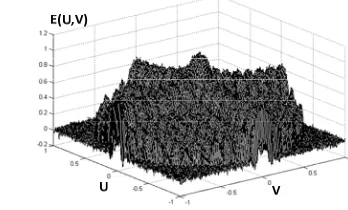
In order to construct models in weak noise environment, the noise with 0 and 2 0.064 of Gaussian distribution is added in the training data. According to the steps in section 5.4, we set the RMSE=0.01, let the wavelet network and the improved RBF network learn from the noisy data respectively, and get the results which is shown in Figure 5 and 6.
[image:6.612.328.502.187.292.2]
Figure 5. Estimation of wavelet network. Figure 6. Estimation of RBF network. Fig.5 describes the estimation of wavelet network and Fig.6 describes the estimation of RBF network. From the two pictures we can get that both the wavelet network and the RBF network can estimate the target function well while in weak noise environment.
Constructing Model in Strong Noise
In order to construct the model in weak noise environment, the noise with 0 and 2 0.064 of Gaussian distribution is added in the training data. Set the RMSE=0.02, the training course is similar to that of learning from weak noisy data, and we can get the result which is shown in Figure 7 and 8.
Fig.7 describes the estimation of wavelet network and Fig.8 describes the estimation of RBF network. From the two pictures we can find that the accuracies of two kinds of networks are both decreased with the increase of noise, but the RBF network decreases more obviously.
[image:6.612.117.503.474.583.2]
Figure 7. Estimation of wavelet network. Figure 8. Estimation of RBF network. From the two simulations, we know that both two networks can construct a accurate model in weak noisy environment. But with the increase of noise, the estimation capability of RBF network decreases rapidly while the estimation capability of wavelet network also stay in a high level.
Summary
method and robust to the noise.
Acknowledgement
This research was financially supported by “the Fundamental Research Funds for the Central University”.
References
[1] Bo Wu, Peng-yuan Liu, Zhi-hui Zhang. Research and Simulation of the spatial distribution of radiated electromagnetic field of phased array antenna [J]. Computer Simulation, 2015, 32(12):146-151
[2] Sébastien Lambot, Frédéric André. Full-wave modeling of near-field radar data for planar layered media reconstruction [J]. IEEE Transactions on Geoscience and Remote Sensing, 2014, 52(5): 2295-2303.
[3] Li-cheng Jiao, Shu-yuan Yang, Fang Liu. Seventy years of neural network: review and Prospect [J]. Journal of Computer Science,39(8):1697-1716.
[4] Zhi-jie Chen, Yong-zhen Li, Huan-yao Dai. Modeling and real-time simulation of phased array antenna pattern [J]. Computer Simulation,2011, 28(3): 31-35.
[5] Z. Jun, G.G. Walter, Y. Miao. Wavelet neural networks for function learning [J]. IEEE Trans. Signal Process, 1995, 43(6): 1485-1496
[6] Zhiguo Zhang. Learning algorithm of wavelet network based on sampling theory [J]. Neurocomputing, 2007, 71(3): 244-269
[7] Bassem R. Mahafza, Atef Z. Elsherbeni. MATLAB simulation of radar system design [M]. Electronic Industry Press, 2009.