Summing Series Using Residues
by
Anthony Sofo
A Thesis Submitted at Victoria University of Technology
in fulfilment of the requirements for the
degree of Doctor of Philosophy.
School of Communications and Informatics Faculty of Engineering and Science
Victoria University of Technology Melbourne, Australia
V
IFTS THESIS 515.243 SOF 30001005475365 Sofo, Anthony
Contents
0.1 Abstract, 5 0.2 Statement 6 0.3 Acknowledgments 7
0.4 Dedication 8 0.5 List of Tables 9 0.6 List of Figures 10 0.7 Summary. 11 1 A review of methods for closed form summation 13
1.1 Some Methods 14 1.1.1 Introduction 14 1.1.2 Contour Integration 16
1.1.3 Cerone's method and extension 17
1.1.4 Wheelon's results 20 1.1.5 Hypergeometric functions 25
1.2 A tree search sura and some relations 28
1.2.1 Binomial summation 28
1.2.2 Riordan 28 1.2.3 Method of Jonassen and Knuth 30
1.2.8 Some relations 38 1.2.9 Method of Sister Celine 40
1.2.10 Method of creative telescoping 41
1.2.11 WZ pairs method 42 2 S u m m i n g series arising from integro-differential-difference equations 45
2.1 Introduction 46 2.2 Method 47 2.3 Biirmann's theorem and application 51
2.4 Differentiation and Integration 54
2.5 Forcing terms 56 2.6 Multiple delays, mixed and neutral equations 58
2.7 Bruwier series 60 2.8 Teletraffic example 60 2.9 Neutron behaviour example 63
2.10 A renewal example 65 2.11 Ruin problems in compound Poisson processes 66
2.12 A grazing system 67 2.13 Zeros of the transcendental equation 68
2.14 Numerical examples 70
2.15 Euler'swork 71 2.16 Jensen's work 73 2.17 Ramanujan's question 75
2.18 Cohen's modification and extension 75
2.19 Conolly's Problem 78 3 Biirmann's theorem 81
3.1 Introduction 82 3.2 Biirmann's theorem and proof 82
3.2.1 Applying Biirmann's theorem 86
3.3 Convergence region 89 3.3.1 Extension of the series 90
4 Binomial t y p e sums. 92 4.1 Introduction 93 4.2 Problem statement 93
4.3 A recurrence relation 94 4.4 Relations between Gfc (m) and Fk+i (m) 100
5 Generalization of Euler's identity. 105
5.1 Introduction 106 5.2 1-dorainant zero 106
5.2.1 The system 106 5.2.2 QR,k (0) recurrences and closed forms 109
5.2.3 Lemma and proof of theorem 17 115
5.2.4 Extension of results 118 5.2.5 Renewal processes 121 5.3 The A;-dominant zeros case 123
5.3.1 The A;-system 123 5.3.2 Examples 126 5.3.3 Extension 127 6 Fibonacci and related series. 129
6.1 Introduction 130 6.2 The difference-delay system 130
6.3 The infinite sum 132 6.4 The Lagrange form 134 6.5 Central binomial coefficients 136
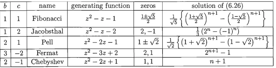
6.5.1 Related results 140 6.6 Fibonacci, related polynomials and products 143
7 A convoluted Fibonacci sequence. 153
7.1 Introduction 154 7.2 Technique 154 7.3 Multiple zeros 157 7.4 More sums 161 7.5 Other forcing terms 162
8 Sums of Binomied variation. 164
8.1 Introduction 165 8.2 One dominant zero 165
8.2.1 Recurrences 166 8.2.2 Proof of conjecture 169
8.2.3 Hypergeometric functions 172
8.2.4 Forcing terms 175 8.2.5 Products of central binomial coefficients 176
8.3 Multiple dominant zeros 179 8.3.1 The A; theorem 180 8.3.2 Numerical results and special cases 183
8.3.3 The Hypergeometric connection 184
8.4 Non-zero forcing terms 185 8.5 Appendix A: A recurrence for Q's 187
8.6 Appendix B: Zeros 190 Conclusion and suggestions for further work 195
0.1 Abstract.
This thesis deals with the problem of representation of series in closed form, mainly by the use of residue theory. Forced differential-difference equations of arbitrary order are considered from which infinite sums of the form
Si(R,k,b,a,t) = ^^y . J (r.k^Rk-.y. '
with arbitrary parameters (R, k, b, a, t), are generated. For the most basic case of
(R, k) = (1,1) the infinite sum ^i (1,1,6, a, t), in different form, has been considered by various
mathematicians including Euler, Jensen and P6lya and Szego. Their methods of representing 5"! (1,1, b, a, t) in closed form are different than those developed by the author; moreover the au-thor demonstrates that Si (1,1,6, a, t) has many appUcations in a wide area of study including teletraffic theory, neutron behaviour, renewal processes and grazing systems. The author proves that for the general case, ^i (R, k, 6, a, t) may be represented in closed form which depends on
k dominant zeros of an associated transcendental characteristic function.
In a similar vein, arbitrary order forced difference-delay equations are considered, from which infinite sums of the form
,^ f r-^R-l\ f n-akr \ . „. ^,
S2(R,k,b,a,n) = J2\ U^-akr-Rk+l^ r.=o \ r J \kr-\-Rr-l J
with arbitrary parameters {R,k,b,a,n) are generated. It is shown that the finite form,
S2F(R,k,b,a,n), of S2{R,k,b,a,n) is associated with Fibonacci and other related
0.2 Statement.
To the best of my knowledge and belief this thesis does not contain any material previously published or written by another author, except where due reference is made in the text. This thesis has not been submitted for any other degree or diploma, at any tertiary institution.
0.3 Acknowledgments.
It is indeed a pleasure to acknowledge the assistance received from my supervisors, Associate Professor Pietro Cerone and Dr. Don Watson. I've been fortunate in being able to spend many hours of constructive discourse with them.
0.4 Dedication.
A mia madre; lei non sa leggere ne scrivere, ma la sua saggezza e
0.5 List of Tables.
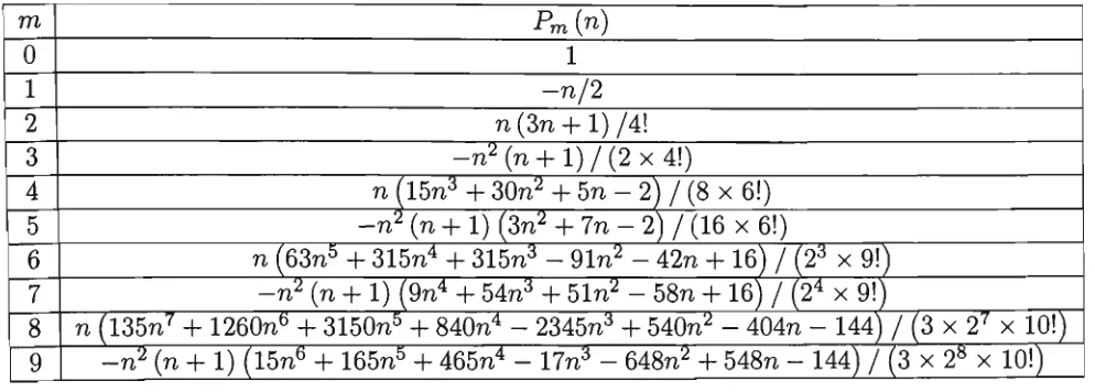
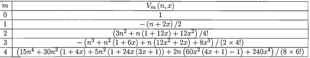
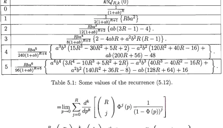
4.1 The beta coefficients of (4.16) 96 4.2 The polynomials of (4.21) 102 4.3 The polynomials of (4.24) 104 5.1 Some values of the recurrence (5.12) 113
0.6 List of Figures.
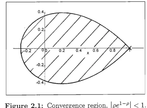
2.1 Convergence region, \pe^ ^| < 1 53
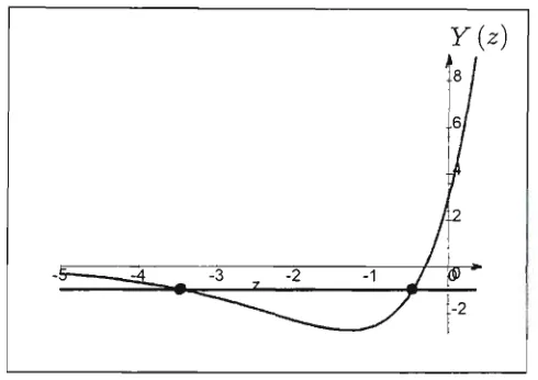
2.2 The contour C, in (2.26) 57 2.3 The real zeros of G(z) defined in (2.49) 69
6.1 Convergence region for the discrete case 133 8.1 The graph of G (2) for a odd or even and 6 > 0. 190
0.7 Summary.
This thesis deals with the problem of representation of series in closed form, mainly by the use of residue theory. Chapter one is a brief overview of some methods; residue theory, recurrences and automated procedures, that are usefully employed in this thesis. Some results given by various authors are generalized and extended. Chapter two develops the techniques, mainly residue theory, that are useful in this thesis. An identity is proved, which has previously been given by Euler and others using different methods than the authors. It it also shown that the particular identity has applications in a wide area of study. Chapter three is concerned with a proof of Biirmann's theorem and the application of the theorem to the identity obtained in chapter two. Some particular finite sums are generated in chapter four and it is proved that they may be represented in polynomial forms, moreover they are gainfully utilized in chapter five. Forced differential-delay equations of arbitrary order are considered, in chapter five, from which infinite sums of the form
Si(R,k,b,a,t) = Y^\ ink + Rk-iy. ^
with arbitrary parameters (R,k,b,a,t), are generated. For the specific case of (R,k) — (1,1),
Si (1,1,6, a, t) reduces to the identity of chapter two. In the general case, the author proves
that Si (R, k, 6, a, t) may be represented in closed form which depends on A; dominant zeros of an associated transcendental characteristic function.
sums of the form
^ ^ f r + R-'^\ f n-akr \ ^ „^^,
S2(R,k,b,a,n) = ^ \ \fJn-akr-m-^-l^ r=o\ r j \kr + Rr-l j
with arbitrary parameters (R,k,b,a,n), are generated. For the special case of {R,k) = (1,1),
S2{1.Ajb,a,n) reduces to the identity obtained in chapter six. By the use of residue theory
Chapter 1
A review of m e t h o d s for closed form
s u m m a t i o n
This chapter consists of two sections. The first section 1.1, is a brief overview of some methods, basically ones dealing with residue theory, which are useful for the summation of series and their representation in closed form. Some results given by various authors are generalized and extended.
1.1 Some Methods
1.1.1 Introduction.
Identities play an important role in mathematics and have been a source of inspiration and sweat for many mathematicians over a long period of time. Jacques Bernoulli (1654-1705), a contemporary of Newton (1642-1722), and Leibniz (1646-1716) discovered the sum of several infinite series in closed form, but did not succeed in finding, in closed form, the sum of the reciprocals of the squares
1 " n = l
"If somebody should succeed", wrote Bernoulli, "in finding what till now withstood our efforts and communicate it to us, we shall be obliged to him". The problem came to the attention of Euler (1707-1783). He found various expressions for the desired sum, definite integrals and other representations, none of which satisfied him. He used the integral representation to compute the sum, S, numerically to seven places, yet this is only an approximate value, his goal was to find an exact value. Euler succeeded, eventually in writing
^ = y - (1-1) Euler [43], moreover wrote "There are many properties of numbers with which we are well
acquainted, but which we are not yet able to prove; only observations have led us to their
knowledge. Hence we see that in the theory of numbers, which is still very imperfect, we can
place our highest hopes in observations; they will lead us continually to new properties which we
shall endeavour to prove afterwards. The kind of knowledge which is supported by observations
and is not yet proved must be carefully distinguished from truth; it is gained by induction as we
usually say. Yet we have seen cases in which mere induction led to error. Therefore, we shall
take great care not to accept as true such properties of numbers which we have discovered by
observation and which are supported by induction alone. Indeed, we shall use such a discovery
as an opportunity to investigate more exactly the properties discovered and to prove or disprove
sense of achievement when Pythagoras (c.580 B.C.-C.500 B.C.) first wrote that for a right angle triangle
2 , „2
a' = b^ + c',
Koecher [69] gave
CO
c(5)
= ^ E
(-1)^
r
i - l .. oo
(-ly
i=i .5 / 2j
Ramanujan, see Berggren [8], evaluated
1 _ 2^v^ y r (4j)!(1103 + 26390J) 7r 9801
3=0 (j!)43964j
Bailey [4] and coworkers wrote, (originally given by Plouffe [75] )
00 ^
j = 0 _8j-M 8j + 4 8i + 5 8i + 6, Amdeberhan and Zeilberger [2] published
c(3)
= E
3=0
(-l)J(i!)^0(205j^-^250j-^77) 64((2j + l)!)5
and Clausen [29] gave the result
2-^1
a,b
a-1-6-I-1/2 re
N 2
> = 3^2
2a, 26, a-h 6 a + 6 + l / 2 , 2 a + 26
X
1.1.2 C o n t o u r I n t e g r a t i o n .
Residue theory and contour integration can be gainfully employed to express certain sums in closed form. From
^ ( - l ) " / ( n ) = - ^ R e s j ( 7 r c s c 7 r 2 / ( 2 ) )
n = - o o j
where Resj are the residues at the poles of / (z), we may obtain some classical residts, namely
^ ^ i i ^ + ^ " 2 ^ [TracothTra - 1] (1.2)
n = l
and
oo ^
TT 2
— coth Tra -f- (TrcosechTra) ^ (n^ -t- a2)2 4a2 a
1 = 1 ^ '
•-The residue evaluation of the integral
27ri / sin 7tz (z"^ -|- 1) leads to the alternating sign identity
^n^ + l 2 VsinhTT /
and also we may obtain
2
a? (1.3)
n=\
A 1 7 r - 3 • ^ sinh^ mt 67r
n = l
Flajolet and Salvy [45] apply contour integral methods to obtain some Euler sums, in particular they recover the alternating term identity, without the use of residue theory
y > ( - 1 ) " ^ h-K^ £ ' o ( 2 n + l ) ^ ~ 1 5 3 6
originally given by Ramanujan
E
, n7 ^ 5 6 7 0 0 ' coth nvr 197r^ n = lThe strength of the Flajolet Salvy paper is that it expenses a method and shows many con-nections of identities with the logarithmic derivative of the Gamma function ip (z), the zeta function, harmonic numbers and double infinite sums. The residts (1.2) and (1.3) are also obtained and extended by Cerone [23] using different methods. The method is described as follows.
1.1.3 Cerone's m e t h o d and extension.
Cerone [23] considers an integral equation of the form
t
B(t) = ^^f^+ j B(t-u)cj^(u)du (1.4)
0
where B (t) is a single sex deterministic model representing births at time t, 0 (t) is a net maternity function which is of compact support and I (x) is the survivor function which gives the probability of surviving to age a; of a newborn. The Inverse Laplace transform of (1.4) is
7+ioo
7—too
where
0 0
T / / N X V{P,X)
and $ ( p ) is the Laplace transform of (j){x). Assuming that $ (p) = 1 has simple roots, pj, which are the only poles in (1.5) then
where
M, =
-oo
d^ip)
P=Pi 0 dp
By allowing (/> (t) to be exponentially constrained Cerone shows that 1 0 ( 0 + )
f e-''Pi(l)(u)du. (1.6)
^ ^ 1 _ MQ + I
and, in general
jP>3 satisfies the recurrence relation
n M\Q ^ ( - l ) " + ' M „ _ f c 6 ' f c , ( - l ) " M n - i . _ , ^ ^ , ( l - M o ) 5 „ = J ^ - — - + ^ - ^ ^ ^ , n = 2,3,4,..., (1.8) ^^^ (n-A;)! ( n - 1 ) ! (1 - Mo)^ where
oo
Mn= u^cj) (u) du <oo
0
oo
f„=y"ux«),
are the n*'* moments of (p (t). Now, in particular if (l)(x) = c6 (x — 6) with c, 6 constants and 5 (x) is the Dirac delta function, then $ (p) = ce~'^ and M„ = c6". The roots of the characteristic equation $ (p) = 1 are given explicitly as
Inc — 27ri7 . „ , . , „
P3 = 1 =^,j = 0 , ± l , ± 2 , . . .
z ^ ; ; 2 — ; 2 = 5 : ; ; 2 l i - ^ « c o t n = l
7ra By considering a partial fraction decomposition, such as
A 1 ^ 1
[f.
1
v ^ _
n = l ln=l n=l
we may obtain, by the use of (1.2) and (1.9), other identities of the form
°° I 1
2_\ —4 4 = -7-4 [2 — Tca(cotna + coth7ta)].
n=l
Taking the limit asa—>^0, in(l.lO), confirms the result
0 0 A
. - 4 TT*
E
n = l
n = 90'
Secondly, (1.2) may also be integrated with respect to the parameter a. From (1.2)
^Al + a
n=\
2a2/7z2_-2 / n 2a2/7z2_-2 da
' f sinh a-K
ln\
(^ ait
}\
(1.9)
(1.10)
(1.11) Integrating both sides of (1.11) with respect to the parameter a and interchanging sum and integral results in
E'"(i
+
^ ) = '
-n = lsinh aTT
aTT
(1.12) where the constant of integration in (1.12) is identically zero. The identity (1.12) is also obtained by Wheelon [91] using a different technique. Notice that the left hand side of (1.12) may be rewritten such that
n(-S) =
sinh a-Kn=\ a-K
The summation of zeros of other transcendental functions have also been considered by several
0 0 0 0
where the m^ are the zeros of the frequency function
g (m) = cos ruj cosh mj-\-l (1.13)
A Taylor series expansion of (1.13) is
, , ^ m^ 2m8 16mi2 iGm^^ I62m20 iQ^m^^
a (m) = 2 ; H 1
^ ^ 6 7! 3.11! 15! 5.19! 24! and since g(m) is an even function in m then -nij and i i m ^ are also zeros of (1.13). If we write
rr / \ V ^ -n ^ f d' i^) Z~°'dz
S(a) = '£m,' = -jllj^^,a>l (1.14)
and choosing a = 4 and a = 8 in (1.14) we recover the two results of Lord Raleigh. From residue
oo
calculations and (1.14) we may also give, for example ^ "^7^^ = ^641 ^^^
j — i *. •'
oo
X) ''^j = 200200ofi2)'^ • -^^o^h^^ operational technique for summing series is that which is described by Wheelon and is worthy of a mention here, since we can generalize some of his results and also make a connection with the polygamma functions, i/^ (x).
1.1.4 Wheelon's results.
Wheelon's method is based on the parametric representation of the general term of a series, so as to produce either the geometric or exponential series inside one or more integral signs. The fundamental operation is contained in the summation of both sides of a Laplace transform pair with respect to a transform variable which is interpreted as the dummy index of summation. This operation exhibits the desired sum as an integral of the geometric or exponential series each of which may be summed in closed form. Consider the Laplace transform of a function
oo
and if we identify the transform variable p with a dummy index of summation n, we can write
oo
'£F(n) = lY,{e-^)^f(x)dx.
(1.15)As an illustration choosing f (x) = x in (1.15), leads to Euler's result (1.1). An obvious extension is that (1.15) may be generalized to
E(f:3.=(^/^'-'-"E(-T/w^^.
(n + a)The integral representation of (1.15) may be so chosen to allow for denominators with rational and irrational algebraic functions and linear factors, and the numerator may be so chosen to allow for algebraic, exponential, trigonometric, inverse trigonometric, logarithmic, Bessel and Legendre functions. The convolution theorem may be beneficially exploited, so that we may write, for j >2
U V
aia2as...aj
= 0-1)!/*/*.../-—
dw
0 0 0
(^' — 1) times
V ^ '
[ai (l — u)-\- Q!2 (u — v)-^ as {v — w)... + ajwY
and using the relation
t-uh^.!'-'^-""^
allows a generalization of Wheelon's result as
sia,j)^j:- = jfrTy. n : ^ ^ ^ "
"=o n («^+k) --"
x=0fc=l
(1.16)
M 3+1^3
1 1 2 3 I ^^ a^ a^ a^ ""•' a l + g 2 + a S+g .7+0
a ' a ' a ' • " ' a
for a G 5R and j = 2,3,4,... . From(1.16) we can see that
•^ J l-x"
x=0
-dx = j+iR
1 1 2 3 i ' a ' o ' a ' •••' a l+g 2+g 3+a j + a
a ' g ' g ' • • • g
Also, for a and j integers > 1 we have, because of symmetry and known properties of the hypergeometric function
3+1^3
1 1 2 3 I 1 a'' ai a'> •"•' a
l+g 2+g 3+0 j+g
o ' g ' g ' •'•' g
= g+l-'^g
•"•' g ' g ' g ' • " ' a
1+2 2+2 3+2 £±i
a ' g ' g ' '•'' a
For specific values of a and j various listings of (1.16) occur in the works of Jolley [64], Hansen [54] and Gradshteyn and Ryzhik [47]. We may also obtain some other interesting cases as follows. From (1.16)
S{1,3) =
a - l ) 0 - - l ) ! j !
- — j+\Fj1,1,2,3, ...,j 2 , 3 , 4 , . . . , i - M and we have the identity, from Gauss's 2i^i summation
2i^l 1,1
J + 1
J - 1; i > 2 .
For a = 2, and from(1.16)
S(2,j) =
(i-1)!
2 ^ - l n 2 4 - g ( - l ) ^ ' ^ ' - ^ ^ ^ ^ " " ^ ( 2 ^ - ^ )
r = l= J,3^lF,
i l i a 2
-^j 2 ' ' 2 ' • • • ' 2
3 9 2+2 2 , ^ , . . . , 2
3i^2
ii,i
1±2 2+2 2 ' 2
j2^
4
J - 2 l n 2 - f ^ ( - l )
, and hence
Other specific values of (1.16) may be obtained as follows
5(6,12) =
15(12!) 61440 In 2 -h 10935 In 3 + 12257r\/3 - 61251
Vl\'^'
1 1 1 1 2 5 -1
•••' 6 ' 3 ' 2 ' 3 ' fi' -•• 6 ' 3 ' 2 ' 3 ' 6
13 7 15 8 17 6 ' 3 ' 6 ' 3 ' 6 ,3
and hence
157^6
1 1 1 1 2 5 1 ' 6 ' 3 ' 2 ' 3 ' 6 ' 13 7 15 8 17 o
6 ' 3 ' 6 ' 3 ' 6 '"^
= 61440 In 2 + 10935 In 3 + 12257r\/3 - 61251.
Non integer values of a may also be considered and hence (1.16) may be related to the polygamma functions. The following two examples are given; 5 (^,8) = g f n ^ ^'^'^ from (1.17) we have 9-^8 1,2,4,6,8,10,12,14,16 3,5,7,9,11,13,15,17 67864 45045' also
S (^,^ = 2 ^ I 3455 - 5607r\/3 - 700In3 -H I263F2
and again from (1.17) we have the identity
5 9 10 3 ' " ^ ' 3
11 13 3 ' 3
1 - 363F2
9 7 8 '^' 3 ' 3
11 13 3 ' 3
1 _
TT 6F5 3
" 1 2 4 9 8 10 ••-' 3 ' 3 ' ' ^ ' 3 ' 3
5 7 0 11 13 3 ' 3 ' * ^ ' 3 ' 3
+ S63F2
0 I 8 ^ ' 3 ' 3
11 13 3 ' 3
- I263F2
5 9 10 3 ' ' ^ ' 3
11 13 3 ' 3
= 3455 - 5607rA/3 - 700 In 3.
Numerical estimates of the integral (1.16) may be determined for those values of a and j which do not permit an analytical solution of the integral;
5" (.1,9) ~ .00001315 = -^ loFg 1,10,20,30,40,50,60,70,80,90 11,21,31,41,51,61,71,81,91
Using this procedure Wheelon also sums the double infinite series
oo oo .. ..
both of which agree with the results obtained by Bromwich [19]. A similar summation proce-dure, to that given by Wheelon, has been developed by MacFarlane [71], which depends upon the properties of the Fourier-Mellin transformation. From Wheelon's work, we may now see a connection with (1.16) and the polygamma functions, ^ (x). From (1.16), let j = 2 and a = ^
, A; G iV in which case we may write, by partial fraction decomposition
4A;2 2^-1
v - ^ 4A; v--r 1
^^ ^ 5 ^ (n + 2fc)(n + 4fc) ^ ^^ | J ^ from which, we obtain the very slow converging series
S'fc = 2A;{V'(4A;)-V(2A;)}.
If
5=E
Z^ n2 (4n2 + 1)we may use partial fraction decomposition with polygamma functions, so that
S = 8 V ( 1 ) - 8 V ' ( ^ ) + V ' ( 1 ) + V ' ' ( ^ )
= 2 + C ( 2 ) - 7 r c o t h ^ .
method may be seen in the books of Jury [66] and Vich [89].
1.1.5 Hypergeometric functions.
Binomial sums and hypergeometric functions are intrinsically related. It is of fundamental importance that binomial sums can be generally written as a terminating hypergeometric series, see Roy [80]. The book, A=B, by PetkovSek, Wilf and Zeilberger [74] expertly expounds the theory of hypergeometric closed form representation of binomial sums. The following is therefore a brief description of the hypergeometric function and some of it's prominent properties. The books of Bailey [6], Slater [82] and Caspar and Rahman [46] cover all of the material presented here.
If the ratio of two consecutive terms Tk+i/Tk , in a series, is a constant, then we have a geometric series. A hypergeometric series arises when the ratio is a rational function of a positive integer A;,
Tk+i ^ (ai + k)... (ap -{-k)z
Tk (bi + k)...(b,-^k)(l + k) ^ • ^
where ai, ...,ap\bi^...,bq and z are complex and TQ — 1. Pochhammer's function is defined as
(«)o = 1
( a ) , = a ( a + l ) . . . ( a + fe-l) = ^ ^
(1.19)
and hence a hypergeometric series may be written as
pFq ai,a2,. bi,b2,.
..,ap ..,bq
1
z
The hypergeometric series (1.20) is symmetric both in its upper parameters ai,...,ap and its lower parameters bi^...,bq. In general it is required that 6i_...,6g ^ 0, — 1, — 2,..., since otherwise the denominators in the series will eventually become zero. If for some j , aj = —n then all terms with k > n will vanish, so that the series will terminate. In the non-terminating case, the ratio test yields the radius of convergence, which is infinite iov p < q -\-1,1 ioi p = q + l and 0 ioT p > q -\-1. Moreover, ii p = q-\-l then there will be absolute convergence for [^l = 1
pure and applied mathematics as well as in science. The excellent survey paper of Andrews [3] puts basic hypergeometric functions in an applicable setting. More recently hypergeometric functions led to the solution of the long standing problem of the Bieberbach conjecture by
oo
deBranges [39]; which shows that ii f (z) = z + Y!, ^n^" is a normahzed univalent analytic
n=2
function in the unit disc, then for each n > 2 one has |an| < n. Some elementary cases of hypergeometric series are
QFQ
\.Fo —a
= e^, and
= (l-z)r
Bessel functions may be expressed in the form
(i)"«^'
a-\-l z"T
r ( a + l)Ja(a;)and the 2-F1 series is the classical Gauss series with Gegenbauer, Chebyshev, Legendre and Jacobi polynomials as terminating cases. It is well known in the theory of hypergeometric functions that the confluent iFi function can be obtained from the Gaussian 2i^i function by a limit process called confluence. The hypergeometric function
g + l ^ g ao,ai , a g
6l,62,...,6g
(1.21)
is called A;— balanced \i z = \ and A; -j- ao + ai -I- ... -f- a^ = 61 -|- 62 -I- ... + bq\ or just balanced if A; = 1; well-poised if 1 -f- ao = ai -|- 61 = ... = aq-\-bq., and very well-poised if it is well-poised and oi = 1 -I- ^ . There are a number of cases where (1.21) with argument z = ±1 can be evaluated in closed form as a quotient of products of Gamma functions. Five of these cases are:
1. the Gauss summation formula 2. Kummer summation formula
4. the well-poised Dixon summation formula, and
5. the 2-balanced and very well-poised Dougall summation formula.
The Gauss summation formula is a limit of the Pfaff-SaalschUtz summation formula, Rum-mer's formula is a limit of Dixon's formula and may also be obtained from Dougall's formida. The Pfaff-Saalschiitz summation formula can be explicitly written as
Y ^ (")fc Wfc ( - ^ ) f c ^ (C - a ) n (C - b)n
^ ( c ) , ( l + a + 6 - c - n ) , A ; ! ( c ) J c - a - 6 ) „ ' in particular i f c = o - f 6 - | - l we have
(«)fc (b), _ (1 + a)„ (1 + 6)„ . (l + a
fc=0 (l + a + b)^k\ (l + a + 6)„n!
Hypergeometric sums are often met in the form of combinatorial sums with binomial co-efficients. Evidently, one hypergeometric sum may have many representations as a sum with binomial coefficients. Saalschiitz's summation, for example, may be written as
a-l-A; —1 \ / c —a — 6-|-n — A; — 1 A; / \ c —a — 6—1
E
fc=0
1.2 A tree sesirch sum and some relations.
1.2.1 Binomial summation.
The sum, with some variations and relations, which we shall explore in detail, arises in the work of Jonassen and Knuth [65] in an algorithm known as tree search and insertion. In particular the sum is
We shall explore (1.22) and survey several methods of finding a closed form solution. We shall compare the analytical techniques of Riordan, Jonassen and Knuth, Gessel, Rousseau, the hypergeometric connection, the generatingfunctionology method of Wilf and the automated approaches of Sister Celine, Zeilberger and the WZ pairs method.
1.2.2 Riordan.
Under the heading of Inverse Relations, Riordan [81] considers the identities
'-=5(:)ff)'(:)-'-(ti- ""
'"=s(-r)ff)'(:)=«
' 2n
Riordan analyses (1.23) and (1.24) by recurrences. Writing gn = 2 ^ \ ) , then
n
2" ' 2n
hn = Y.\ |(-l)*^yfc = 2 - ^ n a n d
fc=o V k
Now p„ = (2 - i ) gn-i and also
^-1 ' n - 1
/ 2 n = / n - l + X ; ( - i r ^ ^ f c + l ,
fc=o \ fc y
n ( / n + / n - l ) = E l "" | ( - l ) ' ^ f c : = / l n .
fc=0 \ fc + 1 / Hence
^ (/n + / n - i ) = /in-1 + fn-1 = ^ / n - 1 -l- (n - 1) fn-2, and therefore
n/n = (n - 1) /n-2, /o = 1, / i = 0. (1.25) From (1.25), we have /2n+i = 0 and
_ 2 n - 1 2 n - 3 2 n - 5 1 .^n /^ " 1 / 2 \ / n - 1/2
•^^" - -^^2^r:r^ 2^^4-2 = ^-^^ [ n ) ^ [ n ' ^^ ^ n - l
= •- ! - . - S - n ( - ^ :
Riordan expands on these ideas and obtains the additional identities
s . : . ( ) • : = ^ r : I
-^ 2n + l \ f-Vs" 2k \ _2n + l / 2n
h[k+i jK^J [k)- 2- [^
Riordan attributes the identities (1.23) and (1.24) to Reed Dawson. Another interesting identity related to (1.23) and which may be evaluated by inverse pair relations is
(-4)^
1.2.3 M e t h o d of J o n a s s e n cuid Knuth.
Jonassen and Knuth [65] consider (1.22) and by algebraic manipidations obtain the recurrence (1.25) as follows. From (1.22)
'• = ' - S ( : : : ) ( T ) " ( :
= '--s(.:,)(-)'(:)"?'
- l \ ^ / 2A;
k
fn-l - 2fn-l + - y ^
""toyk+i
hence
n(fn + fn-d = ± " U ^ ) ' f ' ' )• (1-28)
i S V ^ + 1 ' ^ ^
Replacing n with n — 1 in (1-28) we get
(.-l)a-:+/„-,) = E ( j J ( ^ y ( ^ ; )-/„-:. (1.29)
Subtracting (1.29) from (1.28) we obtain the recurrence relation (1.25) and hence identity (1.26) follows.
1.2.4 M e t h o d of G e s s e l .
This method is given on page 3 of the Greene and Knuth [50] book and is described as follows. Replace A; with n — k, that is change the order of summation, in (1.22) such that
"" ' n \ /-W^-^ I 2n-2k
Let [x'^] f (x) denote the coeflacient of x^ in / (x) , hence
n
[rr^ (1 - 2a;)" = | | (-2)'
y n—k (1 + yf-2« = ( 2n 2fc I ( _ 2 j . ^ |^„, ^k (1 ^ ^)2„-a n — k
and therefore
/n = ( - 2 ^ ) ^ [y1 / (1 + y)'" E p ] (1 - 2x)- ( ( ^ )
But since
when / (x) is analytic, then
^\x']fix)g{y)' = f(giy))
fc=0
/„ = ( - 2 ) - [ y - ] ( l + 2 ; ) 2 n | ^ l _ _ ^ y
( - 2 ) - ' ^ [ y T ( l + y 2 ) " ,
and the solution follows
n
2 "• I I , for n even /n = <( V n/2
0 , for n odd.
1.2.5 M e t h o d of Rousseau.
(1.30)
This method is also described in the book of Greene and Knuth [50] and essentially it identifies the coefficient in a polynomial expansion. From
'i_i^±i)
/7=E ru^r^.+ifand
x
fn = M (x^ + ^)''=[x«](l- i i ± i l ! j " , hence
'-mm:
1.2.6 H y p e r g e o m e t r i c form.
Here we consider a slightly more general version of (1.22) in terms of hypergeometric notation. Let
^ 6A; n
/,(a,6) = E l )(-<
k=o\kl \ k
for a real and 6 integer. The ratio of consecutive terms is
=j:Tk
ifc=0
(1.31)
Tk+i ab^ {k - n)
6 - 1 .
7 = 1 ^
+ ^ )
Tk
(*-i)"('=+^)"n(*+a)
(1.32)
To = 1, and hence from (1.32)
fn (a, 6) = 6^6-1
b - l b - 2 h - 3 1 _ r 7 6 ' 6 ' 6 ' •••' 6 ' "
1 6 ^ b^ _±_
•L, ft_i, 6 - 1 ) •••7 6 - 1
06''
( 6 - 1 ) 6 - 1 (1.33)
moreover, for the relatively simple case of 6 = 1
/ „ (a, 1) = iFo —n a
= (1 - ay
Now, we concentrate on the case of 6 = 2 ; from (1.33)
and a recurrence relation for (1.34) obtained from the Zb algorithm in Mathematica, is
(n + 2)/n+2 + (2n + 3 ) ( 2 a - l ) / „ + i + (n + l ) ( l - 4 a ) / „ = 0, /o(a,2) = l , / i ( a , 2 ) = l - 2 a .
(1.35)
We can see from (1.35) that for two special cases of a = 1/2 and a = 1/4 the recurrence relation (1.35) becomes manageable. From (1.34) let a = 1/2 such that
/n ( 2 ' 2 j = 2-Pl i , - n (1.36)
and replacing A; with n — A; we have
/n(-,2J=To2Fi
-n, —n— n
>^o=Hr
I N ' ' / 2n
n
(1.37)
There is an identity, due to Gauss, see Graham, Knuth and Patashnik [49], which states
2-Fi
Oil,Oi2
a i -I- a2 + 1
= 2F1 2(xi,2oL2 a i -I- 0:2 + ^
(1.38)
hence from (1.38) and (1.37)
/n - ( 2n
n
2F1
-—n -—n 2 ' 2
\ - n
-1 (1.39)
Similarly by Pfaff's reflection law
2F1
Q ! i , a 3 - a 2
0:3
2"^ 2i^l
OCl,OL2
0:3
- 1
we have from (1.37)
Using the classical Gauss formula
2 ^ 1 ai,a2
Q!3
_ r (0:3) r (0:3 - Q i - 0 : 2 ) r(Q:3 - 0:2) T (0:3 -ai)
we obtain from (1.39)
_ / - l y / 2n \ r(i-n)r(i)
(1.40)n such that when n is odd fn = 0 and when n is even
_ 4n W / ( 2 n ) ! y £M2n)! _ 2n / 2n
^ ' " ' ' 2n N-U-nlJ (4n)! " ' I
Also, from (1.35) for a = 1/2 we have that (n -f- 2) fn+2 — {n-\-l) fn = 0 which is identical to (1.25) and hence the Reed Dawson identity follows. For a = 1/4, from (1.34)
fnh.2 =2Fl 1 , - n
and from (1.35) (n -\- 2) fn+2 - l{2n-\- 3) /n+i = 0, hence n - l
f '-'rfP^ + ^\ r ( i + " ) _ g - 2 » ' 2>.
n
also from (1.31) / 2 n ( l / 2 , 2 ) = / n ( l / 4 , 2 ) . For 6 = 3, a recurrence relation, using the Zb algorithm in Mathematica, fn (a, 3) = /n, of (1.31) is
2 (n -h 3) (2n -t- 5) /n+3 + (n^ (27a - 12) + n (135a - 56) -F 168a - 66) fn+2+ 2 (n -h 2) (3n (2 - 9a) - M l - 54a) fn+i + (27a - 4) (n + 1) (n -t- 2) / „ = 0,
/o = l , / i = l - 3 a , / 2 = l - 3 a + 15a2
The recurrence (1.41) does not lend itself to easy closed form evaluations for any special values of a. Returning, briefly, to the identity (1.27), we begin with the general form
gn
(a, 6) = E
fc=0
n
k
(-af
bk
k
(1.42)
and in hypergeometric notation
gn (a, 6) = bFb.
I 6^:2 6 ^ _1 • ^ ' 6 - 1 ' 6 - 1 ' — ' 6 - 1 ' "'
6 - 1 6 - 2 6 - 3 \
b •> b •> b 1 • • • ' 6
a ( 6 - l )
b^ 6 - 1
For 6 = 1, ^„ (a, 1) = fn (a, 1) = (1 - a)^ . For 6 = 2,
gn (a, 2) = 2^1 1,—n a
which has a recurrence relation
2 (2n + 1) gn+i -F (n + 1) (a - 4) p„ + 2 = 0, ^o =
1-In the speciflc case of a = 4, we obtain the identity (1.27), evaluated by Riordan, and it may be easily verifled, utilizing the procedure described by PetkovSek et al. [74], by the rational certiflcate function
A; (1 - 2A;) ^ ^ " ' ^ ) ( „ + l _ j t ) ( 2 n l )
-For 6 = 3, a recurrence relation of (1.42), using the Zb algorithm in Mathematica, is
3 (3n + 4) (3n + 5) pn+2 - 2 (n -f 2) (n (27 - 2a) + 27 - 3a) gn+i+ (4a - 27) (n + 1) (n + 2) ^n - 6 = 0, ^0 = 1,51 = 1 - ^a
1.2.7 S n a k e oil m e t h o d .
This method is described on page 126 of the book by Wilf [93]. Let
/ . ( . ) = E ( ; ) / ( - |
and define F (x,y) = J2 fn (u) x^- Now replace for fn (y) and interchange the order of
sum-n>0
mation, such that
f(-,!/)=Ef*V'Ef'' 1-'
fc>0 \ k I n>Q \ k
1 - X ^ I
fc>0 \
2k \ ( xy \^
. . _ ^ k I \ 1 - ^ 2^ ^ . 1
yk 1
(1.44)
Utilizing the identity ^ \ z'^ = , / it follows from(1.44) that fc>0 \ A; ' ^
F(x,y)^
( l _ a ; ) ^ l _ 4 E | ^ ( 1 - ^ ) ( 1 - ^ ( 1 + % ) )
If y = - l / 2 , F ( x , - 1 / 2 ) = -j=^ and the Reed Dawson identity follows. If y = - 1 / 4 , ,2m
F{x,-l/A) = - ^ = E I ^"^ I (f)'"^ and hence, m>o \ rn
n I i ^ - l V f 2A; \ _ ^_^^ j 2n ] r{n + l/2)
fc>0 \ k
^ I : 1 ( T ) : - • > . - - V .
We can generalize (1.43) a little by considering
"" • n \ , I c
and define
F(z,c,b) = Y,fnib,c)z''. (1.46) n>0
Putting (1.45) into (1.46) and interchanging the order of summation, we have
F(.M = E L
h'E, ,
k>0 \ k I n>0 \ k
n
z""
(1 + ^ ( 6 - 1 ) ) ^
zb - ^
( i - ^ r - ^ ' •
For c integer (1.45) will always have a closed form solution, For example, with c = 3, we have
" ' ^Kkin.i
^ ' U N =^(63n3 + 3 6 V ( 3 - 6 ) + 6 n ( l 8 - 9 6 - | - 2 6 2 ) - H 6 ) .
If c = - 1 / 2 and 6 = 2 , we get F (z, -1/2,2) = (l - z^)~^^^ and from the relationship
the Reed Dawson identity follows. If 6 = 1,
•<..-./....=;^=g(:)(i)'.
which corresponds to the Vandermonde identity
1.2.8 S o m e r e l a t i o n s . The related sum
qn
Sn(p,q)='£{-iy
r=0
qn
r
for p and q integers is an interesting one, and is briefiy considered here. For q (1.47) is identical to (1.31) for a = 1 and 6 = 1 . From (1.47) we have
(1.47)
1 and p = I,
Sn (p, q) = pFp-i
and some special cases, from (1.48), are
Sn{l,q)= IFQ
-qn, —qn, —qn,..., —qn
1,1,1,...,1
( - 1 ) P + i (1.48)
-qn
= <
Oifqne Z+
lifqn = 0
and
Sn(p,2) = pFp_i -2n, —2n, —2n,..., —2n
1,1,1,...,! (-1)
P+i (1.49)
. 2n \ 3n \ 2n
It is known that Sn(2,2) = ( - 1 ) " | \, Sn(3,2) = ( - 1 ) ' ' I and therefore
n I \ n ) \ n
5n(3,2) = Sn
n
/S'n(2,2); however for p ^ A, deBruijn [38] showed that (1.49) cannot be expressed as a ratio of products of factorials, and Graham et al. [48] also showed this by an application of the multidimensional saddle point method. We can deduce, from (1.48) the identity
Sn{2,q)= 2F1 —qn, —qn 1
- 1
2gn+l
where B (x,y) is the Beta function. From (1.47) and (1.48) we may also deduce that
(1.50)
2»i+i / 2 n -I- 1
52„+i(p,i)=E(-i)
r=0
= TiFr p - T p - l
- 2 n + 1,...,-2n-t-1
^..(..l)=E(-lrf''')^=(-l^f")^2E(-l)'f-^^
and utiUzing (1.50), gives the new result
yr J nW{l^) 2 ^ „
The sum (1.47) may, for specific cases of p and q, be written as a recurrence relation. Another related sum is given by Strehl [84], whom in an informative paper shows that, for all natural numbers n
= 4-P3
n-{-l,n-\- l,—n,—n
1,1,1 Strehl offers six different proofs of (1.51) based on:
• Bailey's bilinear generating function for the Jacobi polynomials in the special case when the Jacobi polynomials reduce to Legendre polynomials,
• A combinatorial approach to the Bailey identity, • Legendre inverse pairs,
• the Pfaff-Saalschiitz identity, • Zeilberger's algorithm, and
• known recurrences for the Franel and Apery numbers. From (1.51), after various manipulations Strehl obtains
-= 2i^l —n,—n
1
2 + X+\
A (1.53)Given that 2Ai,2 = -S±y/E are the zeros of the quadratic A^ -I- 3A - | - 1 , then from (1.52)
|:(:y<-)-Ef:V^)Ev., ,. a.M)
fc=0 k Al, j=o J
Identifying (1.53) with (1.50) for g = 1 we may also give the identity
n
E I , i
(-1)"
= 2«
fc=o \ A;
and from (1.54) we can write, the new result
—n,—n
1
- 1
2n+l
5(^,lf^)
'"^''H.{:)('^^)tM'^)
where a second order recurrence of (1.54) is (n -f 2) Sn+2 (2,1) -I- 4 (n 4-1) Sn (2,1) = 0, with 5*0 (2,1) = 1 and 5i (2,1) = 0; for n odd Sn (2,1) = 0, hence (n + 1) 5'2„+2 (2,1)-F2 (2n + 1) S2n (2,1) 0 and by iteration S2n (2,1) = {-2)''Y[ ^ •
3=0 ^^
1.2.9 M e t h o d of S i s t e r C e l i n e . Let
where
F (n, k) =
fn = Y,F(n,k)
k=0n \ f-l\^ I 2k
k k
(1.55)
(1.56)
solutions of the recurrence
2 2
E E "^^'J H F(n-j,k-i) = 0. (1.57)
i=0 j=0
utilizing the computer package added to "Mathematica", we can generate the recurrence
2a (n - 1)2 F (n - 2, A; - 2) - (n - 1) {an -2Pn-a)F (n-2,k - 1) -/3n (n - 1) F (n - 2, A;) - a (n - 1) (2n - 1) F (n - 1, A; - 2)
- (2n - 1) (Pn - an - a)F{n - l,k - 1) -hpn(2n - 1 ) F ( n - 1, A;)
-an (n-l)F (n, k - 1) - fin^F (n, k) = 0.
Setting a = 0,P = 1 and summing over A;, we obtain a recursion equation for fn, namely
nfn = in-l) fn-2 , /o = 1, / i = 0
and the Reed Dawson identity follows.
1.2.10 M e t h o d of creative telescoping.
The method of creative telescoping is described in the book of PetkovSek, Wilf and Zeilberger [74]. It utilizes the Zb algorithm in "Mathematica" so that the input
Z6[Binoraial[n, A;] ( — „ I Binomial[2A;, A;], k, n, 2]
responds with a recurrence relation
(1 -h n) Sum[n] - (n 4- 2) Sum[n -F 2] = 0
1.2.11 W Z p a i r s m e t h o d .
This method certifies a given identity as well as having some spin-offs. Given the identity (1.22) we may write
n
^F(n,k) = l (1.58)
fc>0
where
2n \ , i,fc / 2A; ,
( 4 ) . 4"
F(n,k) = ^ ± 2 V k J
(4)^(2fe)!n!^4-' 2n\ (2n-ky.k\^ (4)^(2fe)!n!^4-' (1.59)
n
Calling up the WZ package in "Mathematica" we obtain the certificate function
^ ( - - ^ ) - ( 2 n - . + l K f e - 2 - 2 n ) - ^''''^
G(n,k) = R(n. A;)F(n,A:) = ,, „ \U,^ \ ', ^,. (1-61)
Now, we define
- (-l)^2fc)!n!^ A;!(A;-l)2(2n-A;-h2)!
such that F{n + l,k) — F(n,k) = G(n,k-\-l) — G (n. A;) is true. Sum that equation over all integers k, such that the right hand side telescopes to zero and therefore
J2Firi-hl,k) = Y^F{n,k). (1.62)
ifc>0 fc>o
The two discrete functions F{n,k) and G(n,k) are termed the WZ pairs. From (1.62) and with initial conditions we obtain the Reed Dawson identity. PetkovSek et al. [74] claim that the WZ pairs method provides extra information because of the existence of a dual WZ pair. To obtain the dual WZ pair make the substitution (an -|- 6A; -|- c)! by (_^^_'^fc_^._;^^j for a -I- 6 7^ 0 in (1.59) and (1.61) to obtain F and G. Next change the variables (n,k) by
F* (n, k) = G {—k — 1, —n); G* (n, k) = F (—k, - n — 1), (this transformation maps WZ pairs
to WZ pairs), such that we obtain
F* (. k\ ( - i r ' - ' 2 " ( n - l ) ! n ! 2 ( 2 f c - l - n ) !
and
^ * / M ( - i r ^ ^ 2 " + i n ! 3 ( 2 A ; - 2 - n ) ! , ,
^ ( ^ ' ' ) = 4M2n + l ) ! ( f c - l ) ! 2 • (1-64) As previously, we obtain fn — J2 F* (n, k) and because of the (2A; - 1 - n) term in (1.63) we
fc>0 shall define
/ : = E F*(n,k), (1.65)
fc>[^]
where [x] represents the integer part of x. Now, we need to sum over A;, the recurrence
F* (n + l,k)- F* (n,k) = G* {n,k + l)-G* (n, A:); (1.66)
since the right hand side of (1.66) does not disappear, we sum for A; > 1 -I- [ | ] , this however gives us an extra term, and distinguishing for n odd and n even, we obtain
F* (n + 2,k)- F* (n,k) = G* (n + 1, A; -M) - G* (n + 1, A;) + G* (n,k-\-1) - G* (n,k).
For n even, let n = 2m, and summing for A; > 2 -|- m, we obtain
/* (2 -t- 2m) - / * (2m) + F* (2m,m -f 1) = - G * (2m + l , m + 2) - G* (2m,m -f 2 ) ,
and from (1.63) and (1.64) substituting for F* and G* we obtain
r(2 + 2ra)^ri2rn)+^'"^;'^^'X<'^'f";f. (1.67)
•' ^ / J V / m!(4m-f 3 ) ! ( m - M ) ! Iterating the recurrence (1.67) we have
r ( 2 + 2 m ) - r f 2 ) + V ( 5 a 2 H 2 i ± l ) ! M l ! (1.68) / (2 + 2 m ) - / (2) + ^ j ! ( 4 j + 3 ) ! 0 + l)! ^ '
and from (1.63) and (1.65) we have
/•(2) = - | E ^ ^ - (i«^)
We can put (1.69) in "Mathematica, Algebra, SymboIicSmn" and obtain
r ( 2 ) = l - l n x / 2 . (1.70)
(We may also obtain (1.70) by starting with identity 2.5.16 in the book by Wilf [93]). Now from (1.70), (1.68), and (1.65) we obtain
4 - ( 2 m - l ) ! ( 2 m ) ! 2 ^ ( 2 f c - l - 2 m ) ! ^ 1 ^ ^ ( 3 j + 2) (2;-fl)! (2j)!^
( 4 m - l ) ! ^£^^^ 4fc+iA:!2 ' ^ ^ ' 3 ^ j ! ( 4 j + 3)! (j +1)! " ^ ' ' ' ' ^
Prom (1.67) and (1.70) we also obtain /* (0) = - l n \ ^ and from (1.71) putting k* = k - m and renaming A;* we have the new result
^ (2fc-l)! ^ ( 4 m - 1 ) ! [ ' ^ ^ ( 3 j + 2)(2j + l)!(2j)!2| 4^22fc(m + A;)!2 (2m - 1)! (2m)!2 ] ^ j ! ( 4 j + 3)! (j-Fl)! f"
K—1 ^ 3—" J
Chapter 2
Summing series arising from
int egro- differ ent ial- difference
equations
In this chapter a first order differential-difference equation is considered and by the use of Laplace transform theory an infinite series is generated, which may be represented in closed form. The series, it turns out, arises in a number of areas including teletraffic problems, neutron behaviour, renewal processes, risk theory, grazing systems and demographic problems.
2.1 Introduction.
Differential-difference equations occur in a wide variety of applications including: ship stabiliza-tion and automatic steering [72], the theory of electrical networks containing lossless transmis-sion lines [17], the theory of biological systems [16], and in the study of distribution of primes [90]. The equation
f'(t)+af'(t-a)+Pf(t)+'yf(t-a) + 6f(t-ha) = 0
2.2 M e t h o d .
Consider the first order hnear homogeneous differential-difference equation with real parameters a, 6 and c and real variable t:
(2.1)
(2.2)
(2.3)
f{t) + bf{t)+cf{t-a)=0, t>a
f(t)+bf(t)=0, / ( 0 ) = 1, 0<t<a.
Taking the Laplace transform of (2.1) and using the initial condition, results in
£(f(t)) = F{p) = ^y^UL^i—^ ^
KJKJJ Kf) p^^^^-ap Z . ( p - F 6 ) " + lThe inverse Laplace transform of (2.2) is
n = 0
where the Heaviside unit function
f l , f o r a ; > 0
y 0, for a; < 0.
The solution to (2.1), by Laplace transform theory may be written as 7+ioo
7—too
for an appropriate choice of 7 such that all the zeros of the characteristic function
g{p)=p + h + ce-''P (2.4)
are contained to the left of the line in the Bromwich contour. Now, using the residue theorem
which suggests the solution of / (t) may be written in the form
f{t) = Y^QreP^'
r
where the sum is over all the characteristic zeros pr of g (p) and Qr is the residue of F (p) at
p = pr. The poles of the expression (2.2) depend on the zeros of the characteristic function
(2.4), namely, the roots of g (p) = 0. The dominant zero po of g (p) has the greatest real part and therefore asymptotically f (t) ~ QoeP°* , and so from (2.3),
^ f _l)"c"e~''(*~"'^) (t - anY'
f{t) = Yl - ^ ^ - ^ , ^ ^ H(t - an) ~ QoePoK
n=0 ^
(2.5)
After some experimentation it is conjectured from (2.5) that:
^ (-l)"c-e-^(^—) (t - an)^ ^ ^^^,
n\
n=0
(2.6)
Vf G 5R in the region where the series on the left of (2.6) converges. Biirmann's theorem will be used, a little later, to prove the identity (2.6). By the use of the ratio test it can be shown that the series on the left of (2.6) converges in the region
ace^^"^ < 1 . (2.7)
In a similar fashion, the Laplace transform from (2.2) may be expressed as
„ , , 1 / 6 + c e - « P \ " ^ - ^ ^ l ^ \ (-l)"6"-'-c'-e-«'-P
= 0 r = 0 \ r
and the inverse Laplace transform may be written as
/w-EEf''V'""^""r""''^'"^('-)-^°---
71'As previous it is conjectured that
n ^ ( - i y w ^ - v ; ( t - a r ) " n\
E E r"^^"::'-'''
=QO'^'
(2.8)
n=Or=0 \ r
whenever the double series converges.
Lemma 1 The poles of the expression (2.2) are all simple for the inequality (2.7). Proof: Assume on the contrary that there is a repeated root of
p + 6 + ce-^P = 0 (2.9)
then by differentiation it is required that 1 — ace~°-P = 0, in which case p = In (ac) /a. Sub-stituting in (2.9) results in In (ac) -|- a6 + 1 = 0 and therefore ace^'^"'^ = 1 which violates the inequality (2.7). Hence all the zeros in (2.9) are simple.
Now, the residue Qo of the dominant simple zero po = ^ is
-————-, where (-\-b-hce'"^ = 0, 1 -I- a6 -I- a^
and so the expressions (2.6) and (2.8) become
^ (-l)^c"e-^(*-°^) (t - an)"" _ ^ ^ ( ^ \ (-l)^6"-^c^ (t - ar)"" _ e^'
^ n\ -2^Z^\ ^ ;;:! - l + ab + a^ ^^'^^^
n=0 n = 0 r = 0 \ ^ / i i S
whenever the single and double series converge in a mutual region. Using the transformation
oo n oo oo
EE/(^'^) = EE/(^+^'^) (2.11)
n=0 r=0 n=0 r=0
we obtain, from (2.10)
EE
n n \ r I (n + r)! l + a6 + ae n-\-r \ (-l)"+'-6"c'" (t - ar)'"'^'' e^L e m m a 2
1. The single and double sum in (2.10) are solutions to (2.1) in their region of convergence.
2. The closed form expression in (2.10) is a solution to (2.1) for t > a.
3. The single and double sums in (2.10) are equal in their mutual region of convergence,
which is no larger than that given by (2.7).
Proof: 1. and 2. can be shown to be solutions of (2.1) by substitution and statement 3 of lemma 2 requires that we show
y > A / n \ ( - l ) " 6 ^ - ' ' c ^ ( t - a r ) ^ ^ ^ ^_l)n^n^-b{t-an) (^ _ ^^y
n=Or=0 \ r J ^ ' n=0 n
so that expanding the left hand side and summing each column from the left hand side results
in
cO (t - 0)° 0!
c^ (t - a)^
1!
c^ (t - 2a)^
2!
c3 ( i - 3a)^
3!
l^ b(t-0)^ 6^ (t - 0)^ 63 (t - 0)^
0! "^ 1! ^ 2! ^ 3! "^"
!_ b{t-a)^ 9 (t - a)^ 63 (t - a)^
0! ^ 1! ^ 2! "^ 3! "^
1^ b(t-2af 6^ (t - 2a)^ 6^ (t - 2af
0\^ 1! ^ 2! ^ 3! ^"'
\ b{t-2>af 9 [t - 3a)^ 6^ [t ~ Saf
0 ! ^ 1! ^ 2! ^ 3 ! ^"'
+.
cO(t_o)Oe-''(*-o) c ( t - a ) e - ^ ( * 2 ! l c^ {t - 2af e'^ft-^") c? (t - 3a)^ g-^^^-^a)
0! 1! 2! 3!
=E
(-l^n^n^-bit-an) (j. _ ^ „ ) nn=0 n!
Returning briefly to (2.10), put 6 -|- c = 0, which imphes that ^ = 0, also let t = —ar, so that
E(^)"Er^^"^'<^"^^"-'
n=0 r=0 \ r n\
The inner sum, which we shall generalise in chapter 4, is (-l)"", and hence we obtain the common series
E(-^r = rh^- (2.12)
„ l-l-a6n=0
Biirmann's theorem [92] will now be used to prove the explicit form of relationship (2.6).
2.3 Burmann's theorem and application.
T h e o r e m 3 Let (j) be a simple function in a domain D, zero at a point (3 of D, and let
0(^) ' ^"^ 0'(/3)'
/ / / (z) is analytic in D then "iz G D
f{':)'^f ( « + E ^-^^ [f (*) {«(*)ru+fl»+.
r! dtr=l
where Rn+i = TT^ dj^
2m
JT JC•<l>(u) in fi
/'(t)0'(^)_^^_
/,\ ,1icV^{t)\ (l>{t)-<f>iu)
The V integral is taken along a contour T in D from P to z, and the t integral along a closed
contour C in D encircling T once positively.
We shall prove Biirmann's theorem in chapter three. However next, we shall apply Biir-mann's theorem to equation (2.10).
The characteristic function (2.4) may be shown to have a simple dominant zero at p = 0 for 6 -f c = 0 and 1 + a6 > 0. Thus from (2.6)
^ 6"e-^ft-^") (t - an)"" _ 1
^ n\ " l + a6- ^^-^^^
n=0
Let t = -ar, ab = —p, and hence from above
Identity (2.14) is now shown to be true by applying Btirmann's theorem. Let
/ (-^) = 1 ^ ' ^ (^) = ^ = e ^ <^ (^) = ze-^f (^)^^o = 1,
and we will show, in chapter three, that Rn+i —> 0 as n —> oo. From / (t) = ^ ,
f(t) = e-l^^ +
(1
^ ) - ' ' ( E ( - I + ^ ) ' ' ) .
and so f'{t){9(t)Y = 6*^''+=^)* (t), where ^ (t) = X) (x + l+j)P. The coefficients in this
j=o
expression are the same as those in a Taylor series expansion ^^^^ (0) = {x-\-l-\-j)j\. Now let
Br(t) = '^^~-^i[f'(t){d{t)Y] df
dt r-l
- J{r+x) = e
e*^'"+^)*(t)
(r -I- x)
(r-^x)'-^
r-l I '' M ^(0) (^) ^ (y. + a.)r-2
0
r - l
1 r - l ^ " ( i ) - H . . . + (r + a;)^
2 / V r - - 2
* ' (t) +
*^^-'^ (i)
.,0-1)
+ (r + x)«( "• ^ l*^^-^'(i)
Hence
(r + a;)'-^ I "" M (a; + l) + (r4-a;)
B , (0) =
' ' - 2 ' "" ^ ' ( a ; + 2) + 1
\
(r-\-x)
\
r - 3 J ^ 1 ^ (^ + 3) + ... + (^ + a;)M "" ^ | ( a : + r - l ) ( r - 2 ) !
If we now put y = x -\- r we obtain
Br{0) = y ' ' " ^ ( 2 / - r + l ) - F / - 2 ( r - l ) ( y - r + 2 ) + y ' - 3 ( r - l ) ( r - 2 ) ( y - r + 3)
+... + ( r - l ) ! y ( y - l ) + ( r - l ) ! y
= y ' - i r - l)y'-' + (r - l ) y ^ - i - (r - 1) (r - 2)y^-^ + (r - 1) (r - 2)y^-^
-...-{r-l)\y + {r-l)\y
= y^ = ( x - ^ r ) ^
Hence it follows that
xz
"-1- z ^-^
T=\ r!
{x + '
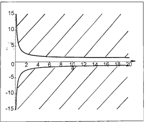
A modification of this siun also appears as a problem in the work of Polya and Szego [75]. By the ratio test the infinite sum (2.14) converges in the region [pe-"-"^! < l,(or |a6e-'^"'"°^| < 1 for (2.13)), and so considering p as a complex variable p = x-\-iy, then (e^^-*^"^) (x^ -f y^)) ^ < 1-The region is shown in figure 2.1.
0.4.
F i g u r e 2 . 1 : Convergence region, \pe^ P\ <1.
On the boundary p = 1, from (2.14), the series
\ -^j — may be shown to diverge.
oo
Consider the divergent series J^ J , then by the limit comparison test lim /'e-(^+")(r+n)" \ ^ ^ n=l n-^oo \ n. J on UtiUzing StirUng's approximation n\ ~ ( ^ ) " y/27m as n -^ oo. The divergence of the above series can also be ascertained from the closed form representation of the right hand side in (2.14).
The characteristic function (2.4) may be shown to have a dominant double zero at p = 0 for 6 -h c = 0 and 1 -I- a6 > 0. From the general theory of linear fimctional differential equations [52] it follows that there exists constants a and /3 such that
lim (f{t)-at) = p.
t—»ooFrom residue theory, the constants a and /5 can be shown to be ^ and | respectively, in which case
t^oo y ^ ^ a J 3 From (2.10) and (2.2) it can be seen that
l i ^ / y . ( - l ) " c - e - K ^ - " " ) ( t - a < \ ^ ^_(,+,), ^^j^f n \ ( - l ) " 6 - - c - t »
"~* \ n = 0 ^ ' / n=Or=0
This result can be ascertained directly from the differential-difference equation (2.1).
2.4 Differentiation and Integration.
Rewriting (2.10) we have that
^ ( - l ) " c " e ° ^ (t - an)"" ^ e^(^+^) ^2 15)
^ n\ l-\-ab-\-a^' ^ ' ^
n=0 ^ Differentiating both sides of (2.15) with respect to t, j times we have
On the left hand side (2.16) put n-j = n* and rename n* = n, also put t + aj = x, then the left hand side becomes
(_^)i y ^ (-l)"c^e-K^-°^) (x - an)^ n = 0
and from (2.15), is equal to
=
{-cy
n\
r,Xi
l-\-ab-\-a^'
but from the characteristic function (2.4), since ^ is a zero
(2.17)
- c = ( 6 + 0 e ' .a? (2.18)
and therefore (2.17) is equal to
(6 + ^)^6=^^ 1 -I- a6 -F a^
which is equivalent to the right hand side of (2.16) after renaming x as t. We may also integrate (2.15) j times such that
E
n=0
( - l ) ^ c " e " ' ' " ( t - a n ) " + ^ '
(n + j ) !
=/ /i
.t(6+0
-I- a6 -h a^ dt. j—times
For j = 1 we have, from (2.19)
E
n=0
( _ l ) n c n g - b ( t - a n ) (^ _ a n ) " + ^
(n + 1)!
ot^
(6 + 0 ( l + a& + O + Ke -bt
(2.19)
(2.20)
where iiT is a constant of integration. Now putting t = x — a,n* = n-hl and renaming the counter n*, we have
E
n = l
( _ l ) n c n e - 6 ( x - a n ) (3. _ ^ ^ ) n
= —C
n!
gf(x-o)
(6 + e ) ( l + a6 + aO + Ke-^^^~°'^
on the right substitute (2.18) for - c , such that K = - ^ ^ ^ . Thus from (2.20)
oo
E
n=Q (n + 1)! ~ " 6-he
M
l-\-ab-\-a4
_ „-b{t+a)-a^ (2.21)
If 6 4- c = 0 and 1 -|- a6 7^ 0 then ^ = 0, in which case from (2.21)
E
n=0
(n + 1)! ~b
_ „-fc(t+a)
l + a6 (2.22)
2.5 Forcing terms.
The result (2.19) may be arrived at by considering a difference-delay equation with a forcing term. Let
f(t)+hf(t)-hf{t-a) =
fn-l^-btr ( m )
,/(o) = o.
(2.23) for m a positive integer. Following the procedure of the previous sections, we haveF(p) =
{P + 6)"" (p + 6 - 6e-°P) (2.24)
where F {p) has a simple dominant pole at ^ = 0, and a pole of order m at p = —6. From these considerations we arrive at the result
00
E
n=0
yn^-b{t-an) (^ _ a „ ) " + " ^
{n-\-7ny.
m—\
6"*(l+a6) • ^
^ ' v=0
+ E Pm,u (-6)
j.m—v—\p—bt
(m-u-iy.
(2.25)where
i^^-Pm,v i-b) = lim d"
p-*-b [dp'^ p + 6 - 6e-"P u = 0,1,2, ...,m — 1.
For m = 1, (2.25) gives the result (2.22), and for m = 3 we have the result
00
E
n=0
lfn^-b{t-an) (^ _ ^^y^+i -6*
63 (1 + a6) 66^^^
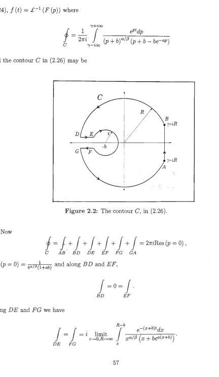
{2.2A),f(t) = £-^{F{p))wheve
7+ioo
7
2m J
eP^dp
7—roo (p + 6)"/^ (p + 6 - 6e-'»P)
and the contour C in (2.26) may be
F i g u r e 2.2: The contour C, in (2.26).
(2.26)
Now
/ = / + / + / + / + / + / = 27riRes (p = 0), c >IB' BD DE EF FG GA
Res(p = 0) = ba//3(i+ab) ^"^ ^^°^§ ^^ ^"^ ^ ^ '
B D EF
Along £)F and F G we have
/ = /
R-b
i limit
e ^ 0 , i l - > o o
J x^.
g-(x+6)t^^
/^ (a; + 6e"(^+^)) '
(2.27)
(2.28)
From (2.27), (2.28) and (2.29)
g - ( x + 6 ) t ^ ^
1_ f 1 1. r e-^''+''>*dx Ini J ~ 6"//3 (1 + a6) ~ TT y W ^ 7 x T 6 e ° ( ^ W ) " '
27ri
A B • x = 0
(2.30)
and if, as previous, our conjecture is to follow then
^ n g - b ( t - a n ) (^ _ ^ ^ ) n + | 1 1 7 e - ( ^ + ' ' ) M x oo j.n_—oir—am fj. \ " - r - 3 i i
^ r
n=0 1
^ - ° " H ^ - a r i ) " " ^ _ . 1 1 /• e-^^+^^Mx
f ^ + a + l " ) • 6 ° / / ' ( l + a 6 ) 7r 7 x ° / ^ (x + 6e°(^+'')) ^ ' '^
\ P } x=0
however, since the integral in (2.30) is improper and divergent then (2.31) is not an identity. A similar improper divergent integral (2.30) may be obtained for any real number m.
2.6 Multiple delays, mixed and neutral equations.
Consider an equation with two delays
f'(t) + bfit-a)-bf(t-p) = 0, f(0) = l,a,P>0. (2.32)
Taking the Laplace transform of (2.32) we obtain
^^^ ~ p + 6e-"P - be-PP
which has a simple dominant pole at ^ = 0. We may write F (p) in series form such that
n=0 P r=0 \ r J
—p(an+/Sj—ar)
and so using the techniques of the previous sections we have
If a = 0 and /? = a (2.32) reduces to (2.1) and (2.33) is equivalent to (2.10). I£ p =-a (2.32) becomes a mbced equation, and (2.33) reduces to the identity
E(-rE(-ir
' n \ {t-a{n- 2r))"n=o r=o \ r J ^- l-2ba'
For the homogeneous neutral equation (forcing terms may also be added).
f'(t)+bf'(t-a)+cf(t-a) = 0, f{0) = l
we obtain
F(p)= ^ p + pbe-°'P + ce-'^P'
and from the methods of the previous sections
V y " r - 6 r ( " ^ (<'Yi*-^'>^T ^ (c + bQe^
h h [rJ^bJ r! c - a e ( c - 6 0 '
where ^ is the dominant zero of the characteristic function
9{p)=P+{c + bp) e-°-P.
Using the transformation (2.11), (2.34) reduces to the identity
\^\^'(-^^r^+r.n^r / ^ + ^ ^ {t-a{n + r)Y _ (c + b^)e'^
h U ^ ^ \ r j rl -c-a^c-bO^
and for the degenerate case of a = 0 we have oo n
n 'cty (-6)" e-'=*/(i+^)
(2.34)
h ^ o [ r n b ) r! 1 + 6
2.7 Bruwier series.
Bellman and Cooke [7] refer to
n=0
as the Bruwier series, see [20] and [21], which is a solution to the advanced equation
/ (t) - ^f (t + oj) = 0, f (0) = 1. (2.35)
Comparing (2.35) with (2.1) it can be seen that 6 = 0, c= -u, a = -cv and from the series at (2.11)
y r z ^ " ( t + na;)" _ e^' ^ n! " l - a ; ^ '
n=0 ^
where ^ is the dominant real root of ^ - ve'^^ = 0 and \i^Loe\ < 1, is the region of convergence of the series.
2.8 Teletraffic example.
Erlang [40], see also Brockmeyer and Halstrom [18], considers the delay in answering of tele-phone calls. The problem is to determine the function / (t), representing the probability of the waiting time not exceeding time t. Hence for an M/M/1 regimen, Erlang shows
oo
/ W = y f(t + y-a)e-ydy.
y=0
real root distribution:
• One root ai p = 0 ioi a < 0,
• one negative root, plus p = O f o r O < a < l ,
• a double (repeated) root at p = 0 for a = 1 and, • one positive root, plus p = 0 for a > 1.
The following results apply for all real values of t , in the region of convergence lae^"*"! < 1.
y > ( - i r e ^ - ° " f t - a n ) - - _ f i z g ^ for a > 1 n=o " ' I y ^ for a < 1 which on putting t = -ar, we may write
y(ae-r{r + n)- _ i f ^ for a > 1
; S ^' \ f^ fora<l
where ^ is the positive dominant root of ^ — 1 + e""^ = 0. Erlang considered only the case of 0 < a < 1. In the case when a = 1 there is a double pole which results in, from a previous statement in section 2.3
lim (f(t)-2t) = l. (2.36)
t—»oo o
This fact has also been noted, in a different context, by Feller [44]. Bloom [12] proposes the prob-lem of evaluating lim ( / (t) — 2t) given that, for t a positive integer f (t) = Y) (-1) e ~"(t-n) ^
*-*°° 0<n<f
The W.M.C. problems group [94] and Holzsager [60] both solve this problem, and in partic-ular Holzsager considers / ( t ) , V t > 0. Now, f (t) satisfies the differential-difference equation
f (t) = f(t) — f (t — I), t > 1 and using the theory of linear functional differential equations,
Holzsager shows the result (2.36). Holzsager's work relates only to the asymptotic of the fi-nite sum whereas in this chapter it is shown that the infifi-nite sum is equal to the asymptotic expression for all t. We may also prove (2.36) in the following way.
T h e o r e m 4