Support Vector Regression Integrated with Fruit Fly Optimization Algorithm for River Flow Forecasting in Lake Urmia Basin

1

Support vector regression integrated with fruit fly optimization algorithm

1

for river flow forecasting in Lake Urmia basin

2

Saeed Samadianfard1_{, Salar Jarhan}2_{, Ely Salwana} 3 _{, Amir Mosavi} 4,5,6 _{,Shahaboddin Shamshirband} 7,8*

3

1 _{Department of Water Engineering, Faculty of Agriculture, University of Tabriz, Tabriz, Iran}

4

2 _{Department of Hydrosciences, Technische Univeristät Dresden, Dresden, Germany}

5

4 Centre for Accident Research Road Safety-Queensland, Queensland University of Technology, Brisbane QLD 4059,

6

Australia;

7

5 School of the Built Environment, Oxford Brookes University, Oxford OX3 0BP, UK

8

6 Institute of Automation, Kando Kalman Faculty of Electrical Engineering, Obuda University, Budapest 1034,

9

Hungary

10

11

7Department for Management of Science and Technology Development, Ton Duc Thang University, Ho Chi Minh

12

City, Viet Nam

13

8Faculty of Information Technology, Ton Duc Thang University, Ho Chi Minh City, Viet Nam

14

15

16

Abstract

17

Adequate knowledge about the development and operation of the components of water systems is of high

18

importance in order to optimize them. For this reason, forecasting of future events becomes greatly significant

19

due to making the appropriate decision. Moreover, operational river management severely depends on accurate

20

and reliable flow forecasts. In this regard, current study inspects the accuracy of support vector regression

21

(SVR), and SVR regulated with fruit fly optimization algorithm (FOASVR) and M5 model tree (M5), in river

22

flow forecasting. Monthly data of river flow in two stations of the Lake Urmia Basin (Vaniar and Babarud

23

stations on the Aji Chay and the Barandouz Rivers) were utilized in the current research. Additionally, the

24

influence of periodicity (π) on the forecasting enactment was examined. To assess the performance of

25

mentioned models, different statistical meters were implemented, including root mean squared error (RMSE),

26

mean absolute error (MAE), correlation coefficient (R), and Bayesian information criterion (BIC). Results

27

showed that the FOASVR with RMSE (4.36 and 6.33 m3/s), MAE (2.40 and 3.71 m3/s) and R (0.82 and 0.81)

28

values had the best performances in forecasting river flows in Babarud and Vaniar stations, respectively. Also,

29

regarding BIC parameters, Qt-1 and π were selected as parsimonious inputs for predicting river flow one month

30

ahead. Overall findings indicated that, although both FOASVR and M5 predicted the river flows in suitable

31

accordance with observed river flows, the performance of FOASVR was moderately better than the M5 and

32

periodicity noticeably increased the performances of the models; consequently, FOASVR can be suggested as

33

the accurate method for forecasting river flows.

Keywords: River flow forecasting; Optimization; M5 model tree; Support vector regression; Fruit fly

35

optimization algorithm

36

37

38

1. Introduction

39

Dependable approximation of discharge is imperative in water resources management (Onyari and Ilunga,

40

2010). Nowadays, stream flow predicting is a dynamic and active research zone which has been studied. The

41

stream flow is censorious to numerous actions such as planning and designing flood protections for farming

42

lands and urban areas, and evaluating the amount allowable extracted water from a river for irrigation (Ismail

43

et al., 2010). By happening a dynamic climate change and continues altering of environmental situations,

44

instantaneous approaches based on utilizing real past data rather than the hydrology of the catchments has

45

become more applicable (Fernando et al., 2012).

46

Generally, data mining is an influential novel methodology based on the abstraction of concealed information

47

from huge data. These tools forecast forthcoming movements of a special system using knowledge-driven

48

decisions resulted from enormous input-output data. M5 model tree (M5), as a sub-technique of data mining,

49

constructs tree based linear models for continues data. Lately, the implementation of M5, as decision tree based

50

regression method, have been stated for hydrological and water-related studies (Bhattacharya and Solomatine,

51

2005, 2006; Khan and See, 2006; Siek and Solomatine, 2007; Stravs and Brilly, 2007; Samadianfard et al.,

52

2014(a,b); Esmaeilzadeh et al. 2017). Londhe and Dixit (2011) implemented M5 to estimate river flow at two

53

stations of India. The models were established by the preceding values of gauged river flow and rainfall for

54

predicting river flow one day beforehand. Sattari et al., (2013) inspected the proficiencies of support vector

55

machine (SVM) and M5 model tree in forecasting flows of Sohu River. They revealed that M5 provided precise

56

predictions comparing with SVM.

57

SVM is a technique in which the strong points of traditional statistical methods, which are theory-oriented and

58

analytically simple, are utilized. SVM approach has been frequently implemented in the areas of hydrology

59

and forecasting time series. Liong and Sivapragasam (2002) applied the method for foreseeing floods. Yu et

60

al. (2004) suggested a method for forecasting daily runoff through combining Chaos Theory and the SVM

61

method. Recently, support vector regression (SVR) method has been developed based on SVM and shows

(ANN) and SVR to monthly streamflow recorded in 2 different stations revealed that both models coupled

64

with wavelet transformation produced more accurate outcomes than the regular models. Also, the results

65

specified that SVR models had enhanced performances comparing ANN models. Wu et al. (2008) used a

66

genetic algorithm to optimize the SVR model, and result exhibited that the suggested model could anticipate

67

river flow precisely in comparison with other models. Londhe and Gavraskar (2015) utilized the SVR model

68

to one-day ahead forecast river flow in two studied locations. The model results were favorable according to

69

the low values of the evaluating metrics.

70

On the other hand, Cao and Wu (2016) coupled Fruit Fly Optimization algorithm (FOA) with SVR (named

71

FOASVR) for optimizing the parameters of SVR. The obtained results exhibited that applying FOASVR had

72

a significant role in increasing the prediction accuracy. Lijuan and Guohua (2016) used FOASVR which

73

hybridizes the SVR model with FOA to estimate monthly incoming tourist flow. It was reported that the

74

suggested FOASVR is a viable option for touristic applications.

75

The key objective of this research is exploiting the accuracy of M5, support vector regression, and optimized

76

SVR with FOA for river flow forecasting in the Vaniar and Babarud stations on the Aji Chay and the

77

Barandouz rivers, respectively, located in the Lake Urmia basin of Iran. Some evaluation parameters for error

78

estimation are utilized for assessing the enactment of the considered models. To the best knowledge of the

79

authors, FOA has not been integrated with SVR in river flow forecasting.

80

81

2. Techniques applied in modeling

82

2.1 M5 model tree

83

With a constant value at their leaves, model trees are based on regression trees (Witten and Frank, 2005). In

84

this regard, M5, as one of the versions of model trees, has a high capability to forecast continuous numerical

85

attributes (Quinlan, 1992). Moreover, two different steps are necessary to develop tree models. Firstly, a

86

splitting principle should utilize for creating a decision tree. This criterion is constructed using the standard

87

deviation (SD) of the class values which reach a node as a size of the error. So, the standard deviation reduction

88

(SDR) is given by:

89

 

 

i

T SD T T T SD

Where T is a set of data that reaches the node and Ti is the ith subset of data. After the first step, data in the

90

secondary nodes have lower SD comparing with initial nodes, so, M5 selects the split which expects to

91

maximize error reduction. Producing a large tree is the main drawback of this step which may cause overfitting

92

problem. Pruning techniques should be employed in order to fix this problem and avoid overfitting. Therefore,

93

the second step for developing M5 involves these techniques and substitution of subtrees with LR functions.

94

As a result, by applying these two steps, M5 develops an LR model for each subspace.

95

96

2.2 Support vector regression (SVR)

97

SVM is recognized as a technique for classification and regression (Vapnik, 1995). Generally,

regression-98

based SVM is called SVR. For solving complex problems effectively, SVR is constructed based on minimizing

99

the structural risk. So, insensitive loss function ( ) identified as the model tolerating errors up to  in the

100

training data. Thus, the SVR pursues a linear function as follows:

101

b x w x

F_{( )} T _{ (2)}

Where w and b represent the coefficients of the weight vector. This can be clarified as the following problem:

102

1

2|| || + (ξ + ξ

∗₎

( ) − ≤ +ξ∗

− ( ) ≤ +ξ

ξ , ξ∗_{≥ 0, = 1,2, … ,}

(3)

Where C>0 is a penalty parameter which has to be selected earlier. The constant C can grade the experimental

103

error. Moreover, ξ ξ∗ which are known as slack variables indicating distathe nce between real values and

104

the corresponding boundary values of _{tube. Hence, in order to minimize Eq. (2) subject to Eq. (3), non-Lthe}

105

R function is given by (Gunn, 1998; Cimen, 2008):

106

 

_











 



N

i

i i

i K x x B

x f

1 *

,

 

(4)

Where

K

(

x

,

x

)

a

,

a



0

107

is an approach which is used to solve this problem by SVR (Smola and Scholkopf, 2004). In this study, the

108

widely implemented kernel named radial basis function (RBF) is utilized for building optimum SVR model.

109

Converging fast, working well in high dimensional spaces and being simple are some advantages of the

110

selected kernel (Wu et al., 2009).

( , ) = exp (− | − | ) (5)

Where is the bandwidth of kernel function. C, andare three predefined parameters. In this research, 1,

112

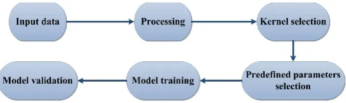
0.01, and 0.001 were selected as default amounts which are used in WEKA software, respectively. Fig. 1

113

indicates scthe hematic configuration of SVthe R model.

114

115

116

Fig. 1 schematic configuration of SVR model.

117

118

2.3. Fruit fly Optimization Algorithm (FOA)

119

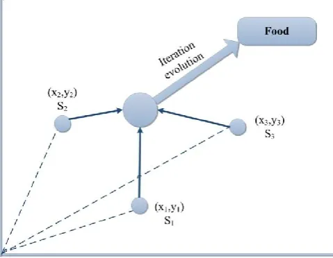
FOA which was introduced by Pan (2012) is a swarm intelligent optimization algorithm that imitates the

120

activities of fruit flies for searching the global optimum. Fruit flies can identify the smell from even 40

121

kilometers and fly on the way to it. Fig. 2 displays the food searching progression utilized by fruit fly

122

iteratively. According to Pan (2012), the following equations are exploited to acquire the initial swarm location

123

of a fruit fly:

124

= ( )

= ( )

(6)

Where LR is the location range of the accidental, initial fruit fly swarm. Subsequently, unexpected search

125

direction and distance for foraging of the fruit flies are given by:

126

= + ( )

= + ( )

(7)

where FR is the random flight range, so, smell concentration judgment value (S) can be computed by:

= 1/ + (8)

128

Fig. 2 food searching process utilized by fruit fly iteratively.

129

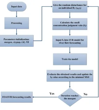
For improving the performance of river flow forecasting, FOA was implemented for choosing optimized values

130

of three SVR parameters including , ε, γ, which are connected to ( , , ) (i.e., = , γ = , and ε =

131

). The flowchart of the mentioned procedure (FOASVR) is displayed in Fig. 3. Moreover, the differences

132

among the predicted and the actual values were evaluated by mean squared error (MSE), as presented in

133

equation belthe ow:

134

=∑ ( − ) (9)

where p and o re the ith predicted and observed values and n is the entire number of data. The fruit fly saves

135

the finest smell concentration value and the corresponding coordinate among the swarms, then flies towards

136

the next place. When the new result is not superior to the previous iteration or the iteration number reaches its

137

maximum, or the error of the prediction reaches the predefined value, this process will stop. Therefore, optimal

138

values are acquired, and the model has the best performance with these values.

140

Fig. 3 The FOASVR flowchart

141

In this research, data were normalized to be between 0 and one because it helps to increase the accuracy of the

142

model and to predict performance (Chang and Lin, 2001). Besides, LR and FR were chosen to be included [0,

143

10] and [-1, 1], respectively; Also, the maximum iteration number (maxgen) was equal to 100, and the

144

population size (size pop) was selected to be 20 in order to have reasonable efficiency. Moreover, Libsvm

145

toolbox was used to run SVR in this article.

146

3. Study area

147

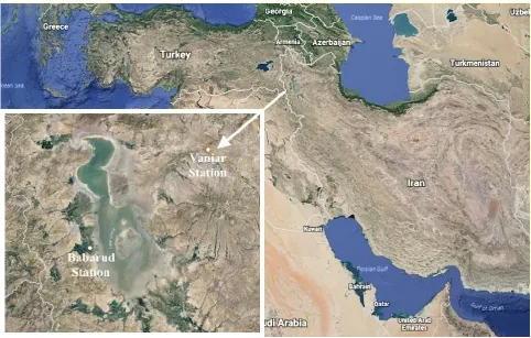
In the current study, the monthly river flow was used for the Vaniar station on the Aji Chay Stream and the

148

Babarud station on the Barandouz River, both located at Lake Urmia basin of Iran (Fig. 4). The observed data

149

include 780 monthly river flows (65 years from 1952 to 2017) for Babarud station and 744 monthly records

150

(62 years from 1952 to 2014) for Vaniar station. Moreover, there is no basic and technical way of separating

151

training and testing data. For example, the study of Kurup and Dudani (2002) used a total of their 63% of data

152

for model development whereas Pal (2006) used 69%, and Samadianfard et al. (2013, 2014) used 67% of total

153

data, and Deo et al. (2018) and Samadianfard et al. (2018) used 70% of total data to develop their models.

Thus, for developing the studied models, the data are divided into training (70%) and testing (30%).

155

Additionally, Table 1 displays the statistics of implemented data for both stations. The observed data confirms

156

high positive values of skewness (Csx = 2.13 and 3.19). Furthermore, the low auto-correlations demonstrated

157

the low persistence for both mentioned stations. According to the crisis of Lake Urmia, the amounts of

158

precipitation and consequently river flow have decreased for the recent years; therefore, this may cause some

159

difficulties in forecasting river flows.

160

161

162

Fig. 4 Babarud and Vaniar stations, located at Lake Urmia basin <URL1>

163

164

Table 1 Statistical parameters of the implemented data (X mean, X max, X min, Sx, Csx, a1, a2, a3 denote the overall mean,

165

maximum, minimum, standard deviation, skewness, lag -1, lag -2, lag -3 auto-correlation coefficients, respectively)

166

Station Data set Xmean

(m3_/s)

Xmax

(m3_/s)

Xmin

(m3_/s)

Sx (m3_/s)

Csx

(m3_/s) r1 r2 r3

Babarud Training data 8.75 66.50 0.00 9.63 2.05 0.70 0.25 -0.07

Testing data 4.71 43.27 0.00 7.37 2.54 0.59 0.14 -0.12

Entire data 7.74 66.50 0.00 9.28 2.13 0.69 0.25 -0.05

Vaniar Training data 14.28 178.29 0.00 21.35 2.94 0.62 0.15 -0.11

Testing data 5.66 65.30 0.00 10.50 3.02 0.50 0.11 -0.05

Entire data 12.13 178.29 0.00 19.58 3.19 0.63 0.18 -0.07

4. Evaluation parameters

168

In this study, different evaluation parameters were considered for scrutinizing the precision of the mentioned

169

models for river flow forecasting.

170

As one of the widely-used statistical parameters, root mean squared error (RMSE) measures the average

171

amount of error (the difference between predicted and observed flows) appropriately, and it can be determined

172

173

 

 







p i Q i

Q n RMSE 1 2 1 (10)

where Qp(i), Qo(i), and n represent the predicted river flow, the observed river flow, and the number of

174

observations, respectively.

175

The bias in the predicted river flow is calculated by the mean absolute error (MAE) which measures the

176

closeness of the predictions to the actual flows. Lower MAE values represent more precise predictions of river

177

flow either equal or close to the observed values. It is calculated as follows:

178

 

 



p i Q i

Q n MAE

1

1 (11)

The correlation coefficient (R), which describes the amount of linearity among simulated and observed values

179

of river flows, ranges from -1 to 1 and is described as follows:

180

   

 

 

 

 

 

 















Also, the Bayesian information criterion (BIC) was utilized to specify the best model parsimoniously which

181

means that the model with fewer input parameters could have better performance in comparison to others. BIC

182

measures models relative to each other; in fact, the model with the best performance has the smallest quantity

183

of the BIC (Burnham and Anderson, 2002). It is given as follows:

184

where K indicates the number of input parameters and RSS can be determined as follows:

 

 









 

n

i

o

p i Q i

Q RSS

1

2 (14)

Furthermore, Taylor diagram (TD) which is a graphical illustration of the observed and forecasted data, was

186

applied for inspecting the precision of models (Taylor, 2001). The TD has this capability to encapsulate some

187

characteristics of the predicted and observed flows at the same time. This diagram can illustrate RMSE, R, and

188

SD between the forecasted and actual data, simultaneously. In TD, the azimuth angle, the radial distance from

189

the origin, and radial distance from the observed data point denote the R-value, the ratio of the normalized SD

190

and the RMSE value of the prediction, respectively.

191

192

5. Results and discussion

193

For evaluating the effects of previous monthly flows, three input combinations were established. Moreover,

194

the periodicity effect was inspected by appending a component π (1 to 12 for each month).

195

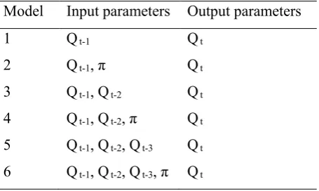
Table 2 Input parameters of the established models.

196

Model Input parameters Output parameters

1 Qt-1 Qt

2 Qt-1, π Qt

3 Qt-1, Qt-2 Qt

4 Qt-1, Qt-2, π Qt

5 Qt-1, Qt-2, Qt-3 Qt

6 Q t-1, Q t-2, Q t-3, π Q t

197

The results of statistical parameters for studied techniques in the test phase for the Babarud station are given

198

in Table 3. As mentioned before, π was appended to the input combinations 1,3, and 5 to examine the effect

199

of periodicity. From the table, it is clear that the periodicity considerably increased each model’s accuracy. For

200

the FOASVR model, R increased from 0.63 (for input combination (1)) to 0.82 (for input combination (2)) and

201

similarly, RMSE and MAE indices decreased from 5.74 to 4.36 and from 3.29 to 2.40, respectively. Regarding

202

two previous cases, by adding periodicity component, R increased from 0.70 to 0.80 and RMSE, and MAE

203

decreased from 5.33 to 4.50 and from 2.90 to 2.67, respectively. Finally, in the case of three previous

204

discharges inputs, R increased from 0.67 to 0.79 and RMSE, and MAE decreased from 5.69 to 4.58 and from

205

3.20 to 2.67, respectively. Comparison of FOASVR, M5, and SVR models indicated that the FOASVR-2

model whose inputs are Qt-1, and π had better accuracy than the M5 and SVR models. M5 also performed better

207

than the SVR model. Overall, FOASVR performed better than SVR and M5s. Also, FOA increased the

208

accuracy of SVR by approximately 27% for RMSE and 38% for MAE in the second scenario which performed

209

roughly (4% RMSE and 14%MAE) better than M5. Without periodicity, FOASVR-3 indicated 6% better

210

performance than M5-3, and they performed better than the SVR-5 model. The relative RMSE and MAE

211

differences between the optimal FOASVR-3 model without periodicity and FOASVR-3 model with periodicity

212

input were 18.2% and 17.2%, respectively. From the BIC point of view FOASVR-2, M5-2, and SVR-4 with

213

the values of 597.55, 581.85, and 701.18 had better performance in comparison with other models which means

214

that these scenarios had parsimonious inputs (accurate result with fewer input parameters), respectively. So,

215

for this station input combination (2) was a reasonable choice. Time variation of observed and predicted river

216

flows by the optimal periodic and non-periodic FOASVR, M5 and SVR models are illustrated in Fig. 5 and 6.

217

It can be comprehended from the figures that all three periodic and non-periodic models considerably

218

underestimate some peak flows. It seems that preciseness of these models decreases with increasing flow rate.

219

However, the superior accuracy of FOASVR and M5 to the SVR model can be comprehended from these

220

figures. Comparison of Fig. 5 and 6 visibly indicate that the periodic models better approximates the observed

221

river flows than the non-periodic models. Fig. 9 displayes the scattered diagrams of the observed and predicted

222

monthly river flows by each method. It is noticeably evident from the graphs that the SVR model performs

223

worse than the other two methods especially in the prediction of peak river flows. Comparison of two figures

224

reveals that the estimates of periodic models are more accurate than non-periodic models. Also, this figure

225

indicates that all models (periodic and non-periodic) overestimate some low flows.

226

The test statistics of the FOASVR, M5 and SVR models for the Vaniar station are also provided in Table 3.

227

Similarly, the encouraging influence of periodicity component on models’ precision is clearly seen for this

228

station. For the FOASVR model, R increased from 0.57 (for input combination (1)) to 0.79 (for input

229

combination (2)) and similarly, RMSE and MAE values decreased from 8.78 to 6.58 and from 4.77 to 3.86,

230

respectively. In the case of two previous discharges inputs, by adding periodicity component, R increased from

231

0.55 to 0.80 and RMSE, and MAE decreased from 8.88 to 6.48 and from 4.97 to 3.75, respectively. Finally, in

232

the three previous discharges inputs case, R increased from 0.55 to 0.81 and RMSE, and MAE values decreased

233

from 8.99 to 6.33 and from 5.53 to 3.71, respectively. Comparison of three models revealed that the optimal

234

and π inputs and both performed better than the optimal SVR-6 model whose inputs are same as FOASVR-6.

236

Generally, FOASVR performed better than SVR and M5 models, moreover, accuracy of SVR was increased

237

by 29.7% and 30.4% related to RMSE and MAE in the optimal scenario (FOASVR-6) by applying FOA,

238

respectively; also, FOASVR showed 16.8% and 19.7% better performances than M5 in terms of RMSE and

239

MAE for this scenario, respectively. Without the periodicity component, the optimal FOASVR-1 model

240

performed better than the optimal M5-1 and SVR-3 model. The relative RMSE and MAE differences between

241

the optimal FOASVR-1 model without periodicity and FOASVR-1 model with periodicity input were 25.1%

242

and 19.1%, respectively. The best values for BIC in this station were related to FOASVR-6 with 703.64,

M5-243

2 with 740.34, and SVR-2 with 825.05. According to the fact that FOASVR-6 was closely followed by

244

FOASVR-4 with the value of 707.09 and FOASVR-2 with the value of 707.53, it is better to choose a

245

combination with fewer input parameters. Thus, the input parameters of Qt-1 and π were selected as a

246

parsimonious scenario for this station similar to the previous station. Fig. 7 and 8 demonstrate the time variation

247

of observed and predicted river flows by the optimal periodic and non-periodic FOASVR, M5 and SVR

248

models. As found for the Vaniar station, here also the three periodic and non-periodic models underestimate

249

some peak flows. Comparison of Fig. 7 and 8 confirm that appending the periodicity component as the input

250

increases the estimation capacity of the models. The scatterplots of the observed and predicted monthly river

251

flows by each method are shown in Fig. 9. Alike to the previous station, the FOASVR and M5 perform better

252

than the SVR model especially in the prediction of peak river flows. This figure indicates that the estimates of

253

periodic models are more accurate. According to Fig. 9, same as Babarud station, the models overestimate low

254

flows in the Vaniar station, so, forecasting shifts from overestimation to underestimation with increasing flow

255

rate.

256

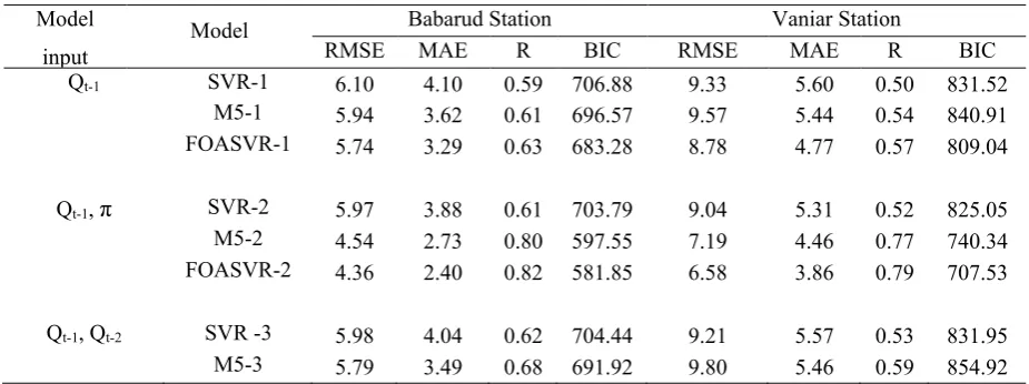
Table 3 The evaluation parameters of studied models in the test period

257

Model

input

Model Babarud Station Vaniar Station

RMSE MAE R BIC RMSE MAE R BIC

Qt-1 SVR-1 6.10 4.10 0.59 706.88 9.33 5.60 0.50 831.52

M5-1 5.94 3.62 0.61 696.57 9.57 5.44 0.54 840.91 FOASVR-1 5.74 3.29 0.63 683.28 8.78 4.77 0.57 809.04

Qt-1, π SVR-2 5.97 3.88 0.61 703.79 9.04 5.31 0.52 825.05

M5-2 4.54 2.73 0.80 597.55 7.19 4.46 0.77 740.34 FOASVR-2 4.36 2.40 0.82 581.85 6.58 3.86 0.79 707.53

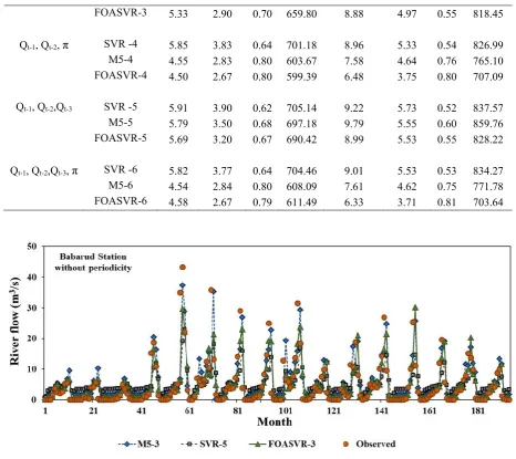
FOASVR-3 5.33 2.90 0.70 659.80 8.88 4.97 0.55 818.45

Qt-1, Qt-2, π SVR -4 5.85 3.83 0.64 701.18 8.96 5.33 0.54 826.99

M5-4 4.55 2.83 0.80 603.67 7.58 4.64 0.76 765.10 FOASVR-4 4.50 2.67 0.80 599.39 6.48 3.75 0.80 707.09

Qt-1, Qt-2,Qt-3 SVR -5 5.91 3.90 0.62 705.14 9.22 5.73 0.52 837.57

M5-5 5.79 3.50 0.68 697.18 9.79 5.55 0.60 859.76 FOASVR-5 5.69 3.20 0.67 690.42 8.99 5.53 0.55 828.22

Qt-1, Qt-2,Qt-3, π SVR -6 5.82 3.77 0.64 704.46 9.01 5.53 0.53 834.27

M5-6 4.54 2.84 0.80 608.09 7.61 4.62 0.75 771.78 FOASVR-6 4.58 2.67 0.79 611.49 6.33 3.71 0.81 703.64

258

259

Fig. 5 The observed and forecasted monthly river flows without periodicity for Babarud station

260

261

Fig. 6 The observed and forecasted monthly river flows with periodicity for Babarud station

263

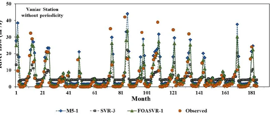
Fig. 7 The observed and forecasted monthly river flows without periodicity for Vaniar station

264

265

266

Fig. 8 The observed and forecasted monthly river flows with periodicity for Vaniar station

269

Fig. 9 The scatterplots of observed and forecasted monthly river flows with and without periodicity for both stations

270

271

Furthermore, TDs were utilized for examining SD and R values for the FOASVR, M5 and SVR models. Fig.

272

10 exhibits TDs for all models, where the space from the reference green point is an amount of the centered

273

RMSE. So, it can be comprehended from Fig. 10 that FOASVR (a point with yellow color) provided relatively

274

precise predictions of river flow in both stations.

275

276

277

Fig. 10. TDs of the monthly predicted river flow

6. Conclusion

281

In the current study, three different data-driven techniques, FOASVR, M5, and SVR were compared in one

282

month ahead river flow forecasting in two stations, located in the Lake Urmia Basin of Iran. Comparison of

283

three periodic models specified that the periodic FOASVR model had better accuracy than the periodic M5

284

and SVR models. M5 was also found to achieve more suitable results than the SVR model. Similar to periodic

285

models, comparison of non-periodic models showed that the optimal FOASVR also had a better performance

286

than M5 and SVR models. It was proved that appending periodicity component significantly increases models’

287

accuracy in forecasting monthly river flows for both stations. For the Babarud station, the relative RMSE and

288

MAE differences between the optimal periodic and non-periodic FOASVR models were found to be 18.2%

289

and 17.2%, respectively. For the Vaniar station, the periodicity component decreased the RMSE and MAE

290

values of the optimal FOASVR models by 27.9 and 22.2%, respectively. According to BIC, the second input

291

combination (Qt-1 and π) opted as parsimonious inputs for FOASVR with values of 581.85 and 707.53 for

292

Babarud and Vaniar stations, respectively. Generally, the performance of FOASVR models was better than

293

the other two methods in forecasting monthly river flows. However, all methods indicated some difficulties in

294

forecasting river flow peaks while the FOASVR models provided a better forecast in high river flows.

295

References

296

Bhattacharya, B., Solomatine, D.P., 2005. Neural networks and M5 model trees in modeling water level–discharge

297

relationship. Neurocomputing. 63, 381–396.

298

Bhattacharya, B., Solomatine, D.P., 2006. Machine learning in sedimentation modeling. Neural Networks. 19, 208–214.

299

Burnham, K.P., Anderson, D.R., 2002. Model Selection and Inference: a Practical Information-theoretic approach, second

300

edition. Springer-Verlag, New York.

301

Cao, G., Wu, L., 2016. Support vector regression with fruit fly optimization algorithm for seasonal electricity consumption

302

forecasting. Energy 115, 734–745. doi:10.1016/j.energy.2016.09.065

303

Chang, C.-C., Lin, C.-J., 2001. Training v-support vector classifiers: theory and algorithms.Neural Comput. 13(9), 2119–

304

47.

305

Cimen, M., 2008. Estimation of daily suspended sediments using support vector machines. Hydrol. Sci. J. 53 (3), 656–

306

666.

307

Esmaeilzadeh, B., Sattari, M.T., Samadianfard, S., 2017. Performance evaluation of ANNs and an M5 model tree in

308

Sattarkhan Reservoir inflow prediction. ISH Journal of Hydraulic Engineering. 1-10.

Fernando, A.K., Shamseldin, A.Y., Abrahart, B.J., 2012. River Flow Forecasting Using Gene Expression Programming

310

Models. 10th _{International Conference on Hydroinformatics HIC 2012. Hamburg, Germany.}

311

Gunn, S.R., 1998. Support Vector Machines for Classification and Regression, Technical Report. University of

312

Southampton, England.

313

Ismail S., Samsudin, R., Shabri, A., 2010. River Flow Forecasting: a Hybrid Model of Self Organizing Maps and Least

314

Square Support Vector Machine. Hydrol. Earth Syst. Sci. Discuss. 7, 8179–8212.

315

Kalteh, A.M., 2013. Monthly river flow forecasting using artificial neural network and support vector regression models

316

coupled with wavelet transform. Comput. Geosci. 54, 1–8. doi:10.1016/j.cageo.2012.11.015

317

Khan, A.S., See, L., 2006. Rainfall-Runoff modeling using data-driven and statistical methods. Institute of Electrical and

318

Electronics Engineers (IEEE).

319

Lijuan, W., Guohua, C., 2016. Seasonal SVR with FOA algorithm for single-step and multi-step ahead forecasting in

320

monthly inbound tourist flow. Knowledge-Based Syst. 110, 157–166. doi:10.1016/j.knosys.2016.07.023

321

Liong, S.Y., Sivapragasam, C., 2002. Flood stage forecasting with support vector machines. J. AWRA. 38 (1), 173–186.

322

Londhe, S.N., Dixit, P.R., 2011. Forecasting Stream Flow Using Model Trees. International Journal of Earth Sciences

323

and Engineering. 4(6), 282-285.

324

Londhe, S., Gavraskar, S.S., 2015. Forecasting One Day Ahead Stream Flow Using Support Vector Regression. Aquat.

325

Procedia 4, 900–907. doi:10.1016/j.aqpro.2015.02.113

326

Pan, W.-T., 2012. a new Fruit Fly Optimization Algorithm: Taking the financial distress model as an example.

327

Knowledge-Based Syst. 26, 69–74. doi:10.1016/j.knosys.2011.07.001

328

Onyari, E., Ilunga, F., 2010. Application of MLP neural network and M5P model tree in predicting streamflow: A case

329

study of Luvuvhu catchment, South Africa. International Conference on Information and Multimedia Technology

330

(ICMT). Hong Kong, China. V3, 156-160.

331

Quinlan, J.R., 1992. Learning with continuous classes. Proceedings Fifth Australian Joint Conf. on Artificial Intelligence

332

(ed. by A. Adams & L. Sterling). World Scientific, Singapore. 343–348.

333

Samadianfard, S., Nazemi, A.H., Sadraddini, A.A., 2014a. M5 model tree and gene expression programming based

334

modeling of sandy soil water movement under surface drip irrigation. Agriculture Science Developments. 3,

178-335

190.

336

Samadianfard, S., Sattari, M.T., Kisi, O., Kazemi, H., 2014b. Determining flow friction factor in irrigation pipes using

337

data mining and artificial intelligence approaches. Applied Artificial Intelligence. 28, 793-813.

338

Sattari, M.T., Pal, M., Apaydin, H., Ozturk, F., 2013. M5 Model Tree Application in Daily River Flow Forecasting in

339

Sohu Stream, Turkey. Water Resources. 40(3), 233-242.

Siek, M., Solomatine, D.P., 2007. Tree-like machine learning models in hydrologic forecasting: optimality and expert

341

knowledge. Geophysical Research Abstracts. Vol. 9.

342

Smola, A.J., Scholkopf, B., 2004. A tutorial on support vector regression. Statistics and Computing. 14(3), 199-222.

343

Stravs, L., Brilly, M., 2007. Development of a low flow forecasting model using the M5 machine learning method.

344

Hydrological Sciences. 52(3), 466–477.

345

Taylor, K.E., 2001. Summarizing multiple aspects of model performance in a single diagram. J. Geophys. Res. Atmos.

346

106, 7183–7192.

347

<URL1>https://earth.google.com/web/@32.205151,53.07029487,2852.42968574a,2667368.97567809d,35y,0.1175398

348

4h,16.72644158t,-0r

349

Vapnik, V., 1995. The Nature of Statistical Learning Theory. Springer Verlag, New York, USA.

350

Witten, I.H., Frank, E., 2005. Data Mining: Practical Machine Learning Tools and Techniques with Java Implementations.

351

Morgan Kaufmann: San Francisco.

352

Wu, C.L., Chau, K.W., Li, Y.S., 2008. River stage prediction based on a distributed support vector regression. J.

353

Hydrol. 358, 96–111. doi:10.1016/j.jhydrol.2008.05.028

354

Wu, C.-H., Tzeng, G.-H., Lin, R.-H., 2009. A Novel hybrid genetic algorithm for kernel function and parameter

355

optimization in support vector regression. Expert Syst. Appl. 36, 4725–4735. doi:10.1016/j.eswa.2008.06.046

356

Yu, X.Y., Liong, S.Y., Babovic, V., 2004. EC-SVM approach for realtime hydrologic forecasting. J. Hydroinf. 6 (3),

357

209–233.

358

Kurup, P.U., Dudani, N.K. Neural networks for profiling stress history of clays from PCPT data. Journal of

359

Geotechnical and Geoenvironmental Engineering 2014; 128(7): 569-579.

360

Samadianfard, S, Delirhasannia, R, Kisi, O, Agirre-Basurko, E. Comparative analysis of ozone level prediction models

361

using gene expression programming and multiple linear regression. GEOFIZIKA 2013; 30:43-74.

362

Samadianfard, S, Sattari, MT, Kisi, O, Kazemi, H. Determining flow friction factor in irrigation pipes using data mining

363

and artificial intelligence approaches. Applied Artificial Intelligence 2014; 28: 793-813.

364

Samadianfard, S., Asadi, E., Jarhan, S., Kazemi, H., Kheshtgar, S., Kisi, O., Sajjadi, S., Abdul Manaf, A., 2018.

365

Wavelet neural networks and gene expression programming models to predict short-term soil temperature at

366

different depths, Soil and Tillage Research, 175: 37-50.

367

Deo, R.C., Ghorbani, M.A., Samadianfard, S., Maraseni, T., Bilgili, M., & Biazar, M., 2018. Multi-layer perceptron

368

hybrid model integrated with the firefly optimizer algorithm for windspeed prediction of target site using a limited

369

set of neighboring reference station data, Renewable Energy, 116: 309-323.