CIRJE Discussion Papers can be downloaded without charge from: http://www.e.u-tokyo.ac.jp/cirje/research/03research02dp.html
Discussion Papers are a series of manuscripts in their draft form. They are not intended for circulation or distribution except as indicated by the author. For that reason Discussion Papers may not be reproduced or distributed without the written consent of the author.
CIRJE-F-452
Implementing Nonparametric and
Semiparametric Estimators
Hidehiko Ichimura University of Tokyo Petra E. Todd Pennsylvania University of December 2006Abstract
This chapter reviews recent advances in nonparametric and semiparametric estimation, with an emphasis on applicability to empirical research and on resolving issues that arise in implementation. It considers techniques for estimating densities, conditional mean functions, derivatives of functions and conditional quantiles in a flexible way that imposes minimal functional form assumptions.
The chapter begins by illustrating how flexible modeling methods have been applied in empirical research, drawing on recent examples of applications from labor economics, consumer demand estimation and treatment effects models. Then, key concepts in semiparametric and nonparametric modeling are introduced that do not have counterparts in parametric modeling, such as the so-called curse of dimensionality, the notion of models with an infinite number of parameters, the criteria used to define optimal convergence rates, and “dimension-free” estimators. After defining these new concepts, a large literature on nonparametric estimation is reviewed and a unifying framework presented for thinking about how different approaches relate to one another. Local polynomial estimators are discussed in detail and their distribution theory is developed. The chapter then shows how nonparametric estimators form the building blocks for many semiparametric estimators, such as estimators for average derivatives, index models, partially linear models, and additively separable models. Semiparametric methods offer a middle ground between fully nonparametric and parametric approaches. Their main advantage is that they typically achieve faster rates of convergence than fully nonparametric approaches. In many cases, they converge at the parametric rate.
The second part of the chapter considers in detail two issues that are central with regard to implementing flexible modeling methods: how to select the values of smoothing parameters in an optimal way and how to implement “trimming” procedures. It also reviews newly developed techniques for deriving the distribution theory of semiparametric estimators. The chapter concludes with an overview of approximation methods that speed up the computation of nonparametric estimates and make flexible estimation feasible even in very large size samples.
Key words
Flexible modeling, Nonparametric estimation, semiparametric estimation, local polynomial estimators, smoothing parameter choice, convergence rates, asymptotic distribution theory
Other key words (less significant)
Additively separable models, index models, average derivative estimator, maximum score estimator, least absolute deviations estimator, semiparametric least squares estimator, trimming, binning algorithms
Implementing Nonparametric and Semiparametric Estimators
1Hidehiko Ichimura and Petra E. Todd November 28, 2006
1Prepared for Handbook of Econometrics Volume 6. This research was supported by NSF grant # SBR-9730688, ESRC grant RES-000-23-0797, and JSPS grant 18330040. We thank Yoichi Arai, James Heckman, and Whitney Newey for helpful comments. We also thank Jennifer Boober for detailed editorial comments.
Contents
1 Introduction 3
1.1 The nature of recent progress . . . 3
1.2 Benefits of flexible modeling approaches for empirical research . . . 3
1.3 Implementation issues . . . 5
1.4 Overview of chapter . . . 6
1.5 Related literature . . . 7
2 Applications of Flexible Modeling Approaches in Economics 8 2.1 Density estimation . . . 8
2.2 Conditional mean and conditional quantile function estimation . . . 9
2.2.1 Earnings function estimation . . . 9
2.2.2 Analysis of consumer demand . . . 10
2.2.3 Analysis of sample selection . . . 11
2.3 Averages of functions: evaluating effects of treatments . . . 12
3 Convergence rates, asymptotic bias, and the curse of dimensionality 12 3.1 Semiparametric approaches . . . 18
3.1.1 Using semiparametric models . . . 18
3.1.2 Changing the parameter . . . 19
3.1.3 Specifying different stochastic assumption within a semiparametric model . . 20
4 Nonparametric Estimation Methods 22 4.1 How do we estimate densities? . . . 24
4.1.1 Moment based estimators . . . 24
4.1.2 Likelihood-based approaches . . . 28
4.2 How do we estimate conditional mean functions? . . . 30
5 Semiparametric Estimation 39 5.1 Conditional mean function estimation with an additive structure . . . 39
5.1.1 Additively separable models . . . 40
5.1.2 Single Index Model . . . 43
5.1.3 Partially Linear Regression Model . . . 45
5.2 Improving the convergence rate by changing the parameter . . . 49
5.3 Usage of different stochastic assumptions . . . 52
5.3.1 Censored Regression Model . . . 53
6 Smoothing parameter choice and trimming 54
6.1 Methods for selecting smoothing parameters in the kernel density estimation . . . . 55
6.2 Methods for selecting smoothing parameters in the local polynomial estimator of a regression function . . . 60
6.2.1 A general discussion . . . 60
6.2.2 One step methods . . . 61
6.2.3 Two step methods . . . 63
6.3 How to choose smoothing parameters in semiparametric models . . . 65
6.3.1 Optimal bandwidth choice in average derivative estimation . . . 65
6.3.2 Other works . . . 67
6.4 Trimming . . . 68
6.4.1 What is trimming? . . . 68
6.4.2 Three reasons for trimming . . . 68
6.4.3 How trimming is done . . . 69
7 Asymptotic distribution of semiparametric estimators 70 7.1 Assumptions . . . 71
7.2 Main results on asymptotic distribution . . . 74
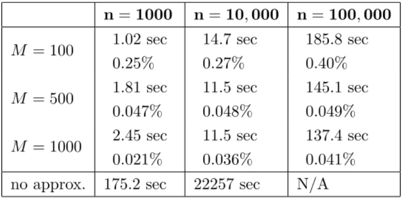
8 Computation 76 8.1 Description of an approximation method . . . 77
8.1.1 A simple binning estimator . . . 77
8.1.2 Fast Fourier transform (FFT) binning for density estimation . . . 78
8.2 Performance evaluation . . . 81
1
Introduction
In the last two decades significant progress has been made in the study of nonparametric and semiparametric models. This chapter describes recent advances with special emphasis on their applicability to empirical research and on issues that arise in implementation. As the coverage of the chapter is broad, and our ability limited, our discussion provides only an overview. It covers mostly cross sectional analysis emphasizing methods which have rigorous theoretical justifications, albeit in most cases only in first order asymptotic forms from frequentists’ view point.1 Nevertheless, we hope the chapter captures the basic motivations and ideas behind the developments and serves as a guide to using the methods appropriately. We begin by briefly summarizing the nature of recent progress, implications for empirical research, and some implementation issues.
1.1 The nature of recent progress
A major motivation for work on flexible models is the desire to avoid masking important features of the data by use of parametric models.2 Recent progress has provided many new ways of modeling and estimating different aspects of a conditional probability distribution. For example, there are now a number of alternatives to linear regression model for modeling and estimating the conditional mean function as well as methods available for examining other features of distributions, such as conditional quantiles. Another area of advance has been in the study of models with limited dependent variables. In the early eighties, the standard approach with such models was to specify the error distribution parametrically and employ parametric maximum likelihood (ML) estimation. Recent research has shown that parametric specification of the error term is often unnecessary for consistent estimation of slope parameters. Models with simultaneity problems can also now be analyzed under weaker functional form assumptions. In these contexts and in others, model specification is beginning to be made more flexible. These developments enable empirical work to be carried out under fewer restrictions than was deemed possible twenty years ago.
Another important motivation for research on flexible models is the pursuit of a classical theme in econometrics: the study of the trade-off between efficiency and allowing for less restrictive models. We often wish to identify a parameter within the broadest class of models possible, but broadening a class sometimes comes at the expense of less efficient estimation. Recent research has clarified the trade-offs in terms of convergence rates and attainable efficiency bounds between specifying more or less restrictive models.
1.2 Benefits of flexible modeling approaches for empirical research
From an empirical perspective, the primary benefit of recent work in flexible modeling is a provi-sion of new estimation methods with a better understanding of the efficiency loss associated with different modeling approaches. Another benefit is that the departure from the traditional linear
1
For developments in studying panel data, see Arellano and Honor´e (2001). 2
modeling framework decreases the tendency to focus on the conditional mean function as the sole object of interest. Using flexible models provides a natural way of considering other aspects of the probability distribution that may be of interest, such as conditional quantiles.3 Research on limited dependent variable models has shown that quantile restrictions provide sharper restrictions than conditional mean restrictions for identifying model parameters.4
When we construct an econometric model of a dependent variable, either explicitly or implicitly, we model the form of a conditional distribution function. Sometimes the conditional distribution function is the parameter of interest, but more often we are interested in particular aspects of it, such as the conditional mean function, conditional quantile function, or derivatives of these functions, as we will see in the next section. When data on the dependent variable given some conditioning variables are directly observed for a random sample of the population, then the nonparametric methods discussed later in this chapter can be directly applied. However, often the application is not straightforward, because the conditional distribution that is observed differs from the conditional distribution in a random population. This can arise in variety of modeling situations, such as with limited dependent variable models, with models with measurement error, and with simultaneity. For example, a demand function can be represented as a conditional distribution of demand given price, but the distribution of the observed quantity-price data may differ from the conceptual conditional distribution we wish to study, because the supply side can affect the observed quantity and price as well.
When the conditional distribution of interest differs from the conditional distribution that can be measured directly from the data, there are two different approaches taken in the literature. One is to search for a source of variation in the data that can be used to identify the conceptual distribution of interest. This may require using data generated from a randomized experiment or from a so-called “natural experiment”.5 When variation of this sort is available in the data, the methods described in this chapter can often be directly applied. An alternative approach is to explicitly model the relationship between the observed distribution and the conceptual distribution of interest and then try to identify some aspects of the distribution of interest from the observed distribution. Much work has been done towards extending nonparametric methods to account for limited dependent variables, sample selectivity, and simultaneity. Section 2.2.3 provides some examples of applications of semiparametric selection models.
An additional benefit of using flexible models is that they allow for a more direct connection between the parameters of interest and the identification restrictions being exploited in estima-tion. For example, consider the linear regression model with the conditional mean restriction
E(y|x) = x0β0. Here β0 represents a vector that defines the conditional mean function and also a vector that defines the derivative of the conditional mean function. Generally, in a restricted framework conceptually different parameters may coincide and there can be a discrepancy between the parameter of interest and the source of variation in the data used to estimate the parameter.
3See e.g. Buchinsky (1995), Chamberlain (1995), Buchinsky and Hahn (1998). 4
Powell (1984), Manski (1985), Chamberlain (1986a), and Cosslett (1987). 5
Using flexible models makes more transparent the source of variation in the data that should be used to estimate the parameter of interest. For example, it is natural to estimate β0 by ordinary least squares when it represents a vector defining the conditional mean function and to estimate it by an average derivative estimator, when it represents a vector defining the derivative of the conditional mean function. Average derivative estimators are discussed below in section 5. Actual implementation may require using a more restricted model for the curse of dimensionality problem we will discuss, however.
Finally, flexible models provide a systematic way of addressing concerns about model specifica-tion. First, they require fewer modeling assumptions, which directly eliminates the need for some specification testing. Second, they provide a formal framework for conducting the specification search. In parametric models, searches often proceed piece-meal, leaving the selection of which models to examine and the order in which to examine them up to the researcher. The route by which a particular model is chosen is often not made explicit, which makes it difficult to obtain general results about the properties of the estimators. Another difficulty is that there is no formal language for effectively communicating the domain of search, and the description of the domain is usually left up to the researcher’s conscious effort. With nonparametric estimators, the class of models for which the estimation is valid is a priori specified, so that the domain is clear and the process by which a particular model is chosen is more transparent.
Careful researchers have always been aware of potential drawbacks of parametric models and have guarded against misspecification by examining the sensitivity of empirical results to alternative specifications and using imaginative ways of checking model restrictions.6 The recent progress in flexible modeling makes it easier for researchers to address concerns about model specification and also to assess the variability of estimation procedures. The progress represents an important step towards replacing what has been characterized as the difficult art of model specification with a simpler, more systematic approach.
1.3 Implementation issues
So far we have emphasized the benefits of using flexible models. To fully realize these benefits, however, there are still some questions that need to be resolved regarding how to choose a model and an estimation method that is well suited to a particular application and how to implement the chosen estimation method.
A key consideration in using a flexible model is that greater flexibility often comes at a cost of a slower convergence rate. Thus, understanding the trade-off between flexibility and efficiency is important to choosing an appropriate estimation strategy. A barrier to implementing the new estimators is how to choose from a bewildering array of available estimators. A first impression from studying nonparametric literature is the richness in the variety of methods. In this chapter,
6
Various formal specification tests and model selection rules have been developed. See for example Davidson and MacKinnon (1981), Hansen (1982), Hausman (1978), Newey (1985, 1987), Tauchen (1985), White (1980), and Wu (1974).
we attempt to pick up some common threads among different methods, to highlight differences and commonalities, and to discuss how each method has been theoretically justified.
Another consideration is that there is a degree of arbitrariness in many of the available estima-tion procedures that takes the form of unspecified parameters. The arbitrariness is not problematic for certain theoretical questions of interest, such as the question of whether a particular level of convergence rate is achievable. But the arbitrariness poses a problem when we implement the method, because different ways of specifying these parameters can greatly affect the estimates. For example, parameter estimates or asymptotic variance estimates can be highly sensitive to the choice of smoothing parameters or to different ways of trimming the data.7 One focus of this chapter is on how to choose the values of these unspecified parameters.
A third problem we address is how to assess the variability of nonparametric and semiparametric estimators. In many empirical applications, the model used and methods applied deviate in some respects from the prototypical models and methods studied in the theoretic literature. Hence, it is important for researchers to be able to modify theories according to their needs and to derive the properties of modified versions of the estimators. For models and estimators based on moment conditions with finite dimensional parameters, Hansen (1982) and Pakes and Pollard (1989) provide results that are sufficiently general to accommodate many different kinds of modifications. For semiparametric models, some progress has also been made along similar lines. See Andrews (1994), and Newey and McFadden (1994) Ai and Chen (2003) and Chen, Linton and van Keilegom (2003), and Ichimura and Lee (2006).
Finally, another obstacle in applying flexible estimators is that they can be computationally intensive, particularly for large data sets. Because of slower rates of convergence, the methods are ideally suited for larger data sets. Yet it is precisely when sample sizes are large, say on the order of 100,000, when the computational burden of these methods can make them impractical. We discuss approximation methods that speed up estimation and provide great gains in speed, making it feasible to analyze even very large samples.
1.4 Overview of chapter
In section 2, we illustrate through examples drawn from different empirical literatures how flexi-ble estimation methods have been used as an alternative or as a supplement to more traditional estimation approaches. Section 3 describes some concepts in semiparametric and nonparametric modeling and makes precise how new developments in the literature broaden the kinds of models and parameters of interest that can be considered in empirical research.
Section 4 discusses nonparametric estimation of densities, conditional mean functions, and derivatives of functions. Although fully nonparametric analysis are not often practical because of slow rates of convergence, we begin with nonparametric estimators because they serve as building
7
“Trimming” is the practice of excluding a fraction of observations in local nonparametric estimation. Trimming is required when the density of the data is low at these observations and a nonparametric estimate would be unreliable. See Section 6.
blocks for many semiparametric estimators. We discuss how apparently different estimators are in some ways closely related and present a unifying framework for thinking about nonparametric density and conditional mean estimators.
Section 5 considers estimation of the same parameters of interest (densities, conditional mean functions, and derivatives of functions) using semiparametric modeling methods that overcome the problem of slow-convergence of fully nonparametric estimators. We describe a variety of semi-parametric approaches to estimating densities and conditional mean functions. Although there are many estimators proposed for a variety of semiparametric and nonparametric models in the literature, we only discuss a subset of them. The models we cover are additively separable models, index models, and partially linear models as well as nonparametric models.
Section 6 focuses on the question of how to choose smoothing parameters and trimming methods in estimators applicable to nonparametric and semiparametric models. The problem of choosing the values of these unspecified parameters is similar to a model selection problem in a parametric context. For each estimator, we summarize existing research on how to choose the values of these parameters and describe the evidence on the effectiveness of various smoothing parameter selection methods, some of which comes from our own Monte Carlo studies.
Section 7 discusses how to assess the variability of different estimation procedures. Section 8 ex-amines the problem of how to compute local nonparametric estimates in large samples. We describe binning algorithms that speed up computation through accurate approximation of nonparametric densities and conditional mean functions.
Section 9 concludes with a discussion of other issues left for future research.
1.5 Related literature
There are many useful surveys in the literature to which we will at times refer in this chapter. For excellent introduction to nonparametric literature in the book form we recommend Silverman (1986) and Fan and Gijbels (1996). Surveys by Blundell and Duncan (1998), H¨ardle and Linton (1994), and Yatchew (1998) cover nonparametric methods compactly. Useful surveys for semiparametric models are given by Arellano and Honor´e (2001), Delgado and Robinson (1992), Linton (1995), Matzkin (1994), Newey and McFadden (1994), Powell (1994), and Robinson (1988).
Books by Bierens (1985), H¨ardle (1990), Prakasa-Rao (1983), Scott (1992) cover nonparametric density or regression function estimation methods. Books by Horowitz (1998), Lee (1996), Pa-gan and Ullah (1999), Stoker (1991), Ullah and Vinod (1993), and Yatchew (2003) cover both nonparametric and semiparametric methods. Deaton (1996) describes how nonparametric and semiparametric models are used in substantively important issues of household bahavior and policy analysis in developing countries.
Efficiency issues are dealt with concisely by Newey (1990, 1993) and in detail by Bickel, Klaassen, Ritov, and Wellner (1993). Most of the probabilistic techniques are explained by van der Vaart (1998) and van der Vaart and Wellner (1996).
2
Applications of Flexible Modeling Approaches in Economics
We first illustrate through several examples how flexible models have been used in empirical work, either as an alternative to more traditional estimation approaches or as a supplement to them. The examples are drawn from the literatures on estimating consumer demand functions, estimating the determinants of worker earnings, correcting for sample selection bias, and evaluating the effects of social programs. Our examples are chosen to highlight different kinds of parameters that may be of interest in empirical studies, such as densities, conditional mean and quantile functions and averages of the functions.
2.1 Density estimation
In many empirical studies, researchers are interested in analyzing the distribution of some random variable. Nonparametric density estimators provide a straightforward way of estimating densities. One nonparametric estimator that has already gained widespread use is the histogram estimator, which estimates the density by the fraction of observations falling within a specified bin divided by the bin width. In section 4, we discuss how the histogram relates to other nonparametric density estimators and how to optimally choose the bin width. We also present alternatives to the histogram estimator that have superior properties, such as the Nadaraya-Watson kernel density estimator for particular choices of kernel functions, which can be viewed as a generalized version of the histogram estimator.
An innovative empirical application of nonparametric density estimation methods is given by DiNardo, Fortin and Lemieux (1996), which investigates the effects of institutional and labor market factors on changes in the U.S. wage distribution over time. DiNardo et. al. (1996) write the overall wage density at time t, fw(w|t),in terms of the conditional wage densities, where conditioning is
on a set of labor market or institutional factors,z, whose effects on earnings they analyze:
fw(w|t) =
Z
Z
fw(w|z, t)fz(z|t)dz.
In their study,zincludes variables indicating union status, industrial sector, and whether the wage falls above or below the minimum wage. Counter-factual wage densities are then constructed by replacingfz(z|t) by a different hypothetical conditional density,gz(z|t), for the purpose of inferring
the effect of changes in elements ofz on the wage distribution.
A traditional parametric approach to simulating wage distributions would specify a parametric functional form for the w and z distributions, in which case inference would only be valid within the class of models specified. The approach taken in DiNardo, Fortin and Lemieux (1996) is to estimate the densities nonparametrically, using a nonparametric kernel density estimator that will be discussed in section 4 of this chapter. Using a flexible modeling approach makes inference valid for a broader class of models and avoids the need to search for an appropriate parametric model specification forfw and fz.
2.2 Conditional mean and conditional quantile function estimation 2.2.1 Earnings function estimation
In addition to studying the shape of the earnings distribution, economists are often interested in examining how changes in individual characteristics, such as education or years of labor market experience, affect some aspect of the distribution, such as the mean. An earnings specification that is widely used in empirical labor research is that of Mincer (1974), which writes log earnings as a linear function of years of schooling (s) and as a quadratic in years of work experience (exp) and other control variables (z):
lny=α0+ρs+β1exp +β2exp2+z0γ+ε.
This simple parametric specification captures several empirical regularities, such as concavity of log earnings-age and experience profiles and steeper profiles for persons with more years of education.8 However, Mincer’s model was derived under some strong assumptions, so it is of interest to also consider more general specifications of the earnings equation such as
lny=g(s,exp, z) +ε,
where g is a function that is continuous in the continuous variable (experience). Usually the g
function is interpreted as the conditional mean function. In Heckman, Lochner and Todd (2005), nonparametric regression methods are applied to estimate the above equation and to examine the empirical support for the parametric Mincer model. Their study finds substantial support for the parametric specification in decennial Census data from 1940-1960 but not in more recent decades.9 Figure 1 shows the nonparametrically estimated log earnings-experience relationship for alternative schooling classes for adult males from the 1960 U.S. decennial census (the same data analyzed by Mincer, 1974). Nonparametric estimation was performed using local linear regression methods that are described in section 4 of this chapter.
{Figure 1: Earnings-Experience Profiles by Education Level Estimated Nonparametrically by a Local Linear Regression Estimator}
One can also interpret the g function to be the conditional quantile function, in which case the nonparametric or semiparametric quantile estimation methods (Koenker and Basset (1978) and Koenker (2005)) can be applied. For example, Buchinsky (1994) applies semiparametric conditional quantile estimation methods to study changes in the U. S. Wage Structure from 1963-1987, using data from the Current Population Survey. He estimates a model of the form:
Y =Xβθ+uθ,
whereβθ is a parameter that characterizes the conditional quantile. The model is estimated under the restriction that theθth conditional quantile of Y givenX =x isx0βθ.
8
See Willis (1986) for a discussion of the use of the Mincer model in labor economics.
9Data from the 1940, 1950, 1960 show support for the model, but data from 1970, 1980 and 1990 show important deviations from the model, which Heckman et. al. (2005) attribute in part to changing skill prices over recent decades, which violates an assumption of the traditional Mincer model.
The estimation yields a time series of the estimated returns to education and experience at different quantiles of the earnings distribution. Buchinsky (1994) finds that the mean returns to education and experience and the returns at different quantiles generally follow similar patterns. Analysis of the spreads of the distributions reveals large changes in the 0.75-0.25 spread and that changes in inequality come mainly from longer tails at both ends of the wage distribution.
2.2.2 Analysis of consumer demand
Several recent studies in consumer demand analysis have made use of flexible estimation techniques in estimating Engel curves, which relate a consumer’s budget share or expenditure on a good to total expenditure or income. Economic theory does not place strong restrictions on functional forms for Engel curves, so earlier research addressed the question of model specification mainly by adopting flexible parametric functional forms. Recent research by Banks, Blundell and Lewbel (1997), Blundell and Duncan (1998), Deaton and Paxson (1998), H¨ardle, Hildebrand and Jerison (1991) and Schmalensee and Stoker (1999), and Blundell, Browning and Crawford (2003) consider nonparametric and semiparametric estimation of Engel curves. The basic modeling framework is
y=g(x, z) +u,
where y is the budget share of a good, x is total expenditure or income, and z represents other household or individual characteristics included as conditioning variables. Typically g(x, z) is as-sumed to be the conditional mean function ofy given x and z so thatE(u|x, z) = 0.
The traditional approach to estimating conditional mean functions specifies the functional form ofgup to some finite number of parameters. In consumer demand analysis, the Engel curve function is often assumed to be linear or quadratic in lnx and z and the coefficients on the conditioning variables are estimated by ordinary least squares (OLS). A nonparametric estimation approach places no restrictions on the g(x, z) relationship other than assuming that the g(·) function lies within a class of smooth functions (such as the class of twice continuously differentiable functions). As discussed in section 3, with a large number of regressors fully nonparametric estimators converge at a rate that is too slow to be practical in conventional size samples. Semiparametric modeling approaches provide a more practical alternative. These methods achieve a faster rate of convergence by allowing some aspects of the g(x, z) relationship to be flexible while imposing some parametric restrictions. For example, the approach taken in Banks, Blundell and Lewbel (1997), Blundell and Duncan (1998), and Deaton and Paxon (1998) is to model the budget-share-log-income relationship nonparametrically under the parametric restriction that otherz covariates enter in a linear, additively separable way. This yields apartially linear model10:
y=g(x) +zγ+u.
Engle, Granger, Rice, and Weiss (1986) considered electricity demand settingx to be the temper-ature andz captures household characteristics. In this application, the parameter of interest was
10
g(x), how the electricity demand peaked as temperature varied. When z are discrete variables, assuming that they enter in a linear fashion imposes only the assumption of additive separability.11 Analogous to the Mincer example, the partially linear model may also be regarded as a conditional quantile function. Blundell, Chen, and Kristensen (2003) has considered the model allowing for endogeneity of income variable.
A variety of semiparametric estimators that allow for flexibility in different model components have been proposed in the econometrics and statistics literatures. Several classes of estimators will be discussed in section 5 of this chapter.
2.2.3 Analysis of sample selection
A leading area of application of flexible estimation methods in economics is to the sample selection problem. In fact, several estimators for the partially linear model were developed with the sample selection model in mind.12 In the sample selection problem, an outcome is observed for a nonrandom subsample of the population and the goal is to draw inferences that are valid for the full population. For example, in the analysis of labor supply the outcome equation corresponds to the market wage, observed only for workers, and the selection equation corresponds to the decision to participate in the labor force. The wage model takes the form
w=w(x, θ1) +u
wherexdenotes individual characteristics,wis observed if the wage exceeds the individual’s reser-vation wage, wr, which is the minimum wage the individual would be willing to accept.
Under sample selection, the above model leads to the wage model of the form:
w=w(x, θ1) +ϕ(x, z) +u
where ϕ(x, z) =E(u|w > wr, x) is the so-calledcontrol function that needs to be estimated along
with parameter θ1.13 Clearly, in the above equation the functions w(x, θ1) and ϕ(x, z) could not
be nonparametrically separately identified without some additional restrictions. Section 5 of this chapter considers alternative estimators for the sample selection model under different kinds of restrictions.
There have been numerous applications of the partially linear sample selection model. For example, Newey, Powell and Walker (1990) and Buchinsky (1998) apply the model to study female labor force participation. Stern (1996) uses it to study labor force participation among disabled workers. Olley and Pakes (1996) use the partially linear model to control for nonrandom firm
11
In more recent work, Ai, Blundell and Chen (2000) consider the consumer demand model of the form
y=g(x+zγ) +zγ+u
and show that including the termzγ both in theg(·) function and in the linear term is necessary to make the Engel curve consistent with a consumer demand system.
12The sample selection model is developed by Gronau (1973), Heckman (1976), and Lewis (1974). 13
exit decisions in a study of productivity in the telecommunications industry. Some additional applications are discussed in section 5.
2.3 Averages of functions: evaluating effects of treatments
A common problem that arises in economics as well as many other fields is that of determining the impact of some intervention or treatment on some measured outcome variables. For example, one may be interested in estimating the effect of a job training program on earnings or employment outcomes.14 In evaluating social programs, the average effect of the program for people participating in it (known as the mean impact of treatment on the treated) is a key parameter of interest on which many studies focus.
Let (y1, y0) denote the outcomes for an individual in two hypothetical states of the world
corresponding to with and without receiving treatment. Let dbe an indicator variable that takes the value 1 if treatment is received and 0 else. The outcome observed for each individual can be written as y = dy1 + (1−d)y0. The mean effect of the program for program participants with
characteristic z is given by E(y1 −y0|d = 1, z). The average of this parameter for the treated
(d= 1) population isE(y1−y0|d= 1).
Clearly the first parameter is more informative than the second. However, as discussed in detail in the next section and in section 6, the conditional onzparameter can be estimated nonparamet-rically less accurately than the second parameter can be estimated nonparametnonparamet-rically.
A variety of estimators have been put forth in the literature to estimate E(y1 −y0|D = 1).
One class of estimators are so-called matching estimators, which impute no-treatment outcomes for treated persons by matching each treated person to one or more observably similar untreated persons. Heckman, Ichimura and Todd (1997, 1998b) develop nonparametric matching estimators that use local polynomial regression methods to construct matched outcomes. Local polynomial regression estimators are discussed in section 4. The application of these estimators in program evaluation settings is considered in this handbook by Abbring, Heckman and Vytlacil.
3
Convergence rates, asymptotic bias, and the curse of
dimen-sionality
A key motivation for developing flexible models is to achieve a closer match between the functional form restrictions suggested by economic theory, which are typically weak, and the functional forms used in empirical work. To study aspects of the conditional distribution functions, such as the conditional mean function and the conditional quantile function, the linear in parameter model is traditionally used. Let the conditioning finite dimensional random vector beX, and aknown finite dimensional vector-valued function evaluated atX =xber(x). Then the linear in parameter model
14See, e.g. Ashenfelter (1978), Bassi (1984), Ashenfelter and Card (1985), Fraker and Maynard (1987), Heckman and Hotz (1989), Heckman and Smith (1995), Heckman, Ichimura, Smith and Todd (1998a), and Heckman, Ichimura, and Todd (1997, 1998b), and Smith and Todd (2001, 2005).
specifies the conditional mean function or the conditional quantile function of a dependent random variable Y by r(x)0θ for some unknown finite dimensional vector θ. For example x = (x1, x2)0
and r(x) = 1, x1, x21, x2, x22, x1·x2
0
. The ordinary least squares (OLS) estimator estimates the conditional mean function and the quantile regression estimator estimates the conditional quantile function. Alternatively, the most flexible model would specify θ(x) for some unknown function
θ(·). The unknown function itself or its derivative could be the parameter of interest.
The specification of parametric models involves two difficulties: which variables to include in the model and what functional form to use. Although nonparametric methods do not resolve the first difficulty, they do resolve the second. Thus if θ(·) could be estimated with the same accuracy as that for the finite dimensional case, then there would be no reason to consider a finite dimensional parameter model. Unfortunately, that is not the case.
Recall that under very general regularity conditions, including the random sampling, most of the familiar estimators–the OLS estimator, the generalized method of moment (GMM) estimator, and the maximum likelihood (ML) estimator–have the property that n1/2(ˆβ −β) converges in distribution to the mean zero random vector with some finite variance-covariance matrix as the sample size n goes to infinity, where ˆβ denotes the estimator and β the target parameter. This implies not only that ˆβ−β converges to 0 in probability, but that the difference is bounded with arbitrarily high probability (i.e. stochastically bounded) even when it is blown up by the increasing sequence n1/2. In this case, we say that the difference converges to 0 with rate n−1/2, that the estimator isn1/2-consistent and that its convergence rate is n−1/2. More generally, if an estimator has the property that rn(ˆβ −β) is stochastically bounded, then the estimator is said to be rn
-consistent or to have convergence rate is 1/rn. Ifrn/n1/2 converges to zero, then thern-consistent
estimator converges toβ slower than the n1/2-consistent estimator does. When two estimators of the same parameter have different convergence rates, the one that approaches to the target faster is generally more desirable asymptotically.15
As discussed, there are estimators of the regression coefficient θ, such as the OLS estimator, that converges with rate n−1/2, so that r(x)0θ can be estimated with the same rate. But in the context of estimating the conditional mean function, Stone (1980, 1982) showed that any estimator of the regression function θ(·) converges slower than n−1/2.
To state the Stone’s results, we need to clarify two complications that arise because the target parameter is a function rather than a point in a finite dimensional spaceRdfor some positive integer d. Note first that we need to define what we mean by an estimator to converge to a function. If we consider a function at a point, then the convergence rate can be considered in the same way discussed above. If we want to consider a convergence of an estimator of a regression function as a whole to the target regression function, then we need to define a measure of distance between two functions. There are different ways we can define the distance between the functions and the discussion about the convergence rate will generally depend on the distance used. Typically a norm is used to define the distance.
15Note that this is an asymptotic statement and the finite sample performance may be different. Clearly, it would also be desirable to have a better understanding about the sample size at which one estimator dominates the other.
To define a few examples of the norms used, letk= (k1, ..., kd) wherekj is a nonnegative integer
for each j = 1, ..., d, and defineDkθ(x) = ∂k1+···+kdθ(x)/∂xk1
1 · · ·∂x
kd
d . Leading examples of the
norms used are the Lq-norm for 1≤q < ∞ (k·kq), the sup-norm (k·k∞), and more generally the
Sobolev norm (k·kα,q ork·kα,∞): X 0≤k1+···+kd≤α Z X D kˆθ n(x)−θ(x) q dµ(x) 1/q or max 0≤k1+···+kd≤α sup x∈X D kˆθ n(x)−θ(x) .
Note thatk·k0,q =k·kq andk·k0,∞=k·k∞.16
Once a norm is defined, then consistency and hence the rate of convergence concept can be defined using one of the three standard consistency concepts, convergence in probability, conver-gence almost surely, and theq-th order moment convergence by how fast the distance between the estimator and the target function converges to 0.17
Which norm is more appropriate will depend on how the estimator is going to be used. For example if a function value at a point or its derivative is of interest, then Lq-norm is not useful because there are many functions close to a function in Lq-sense which does not determine the value at that point or the derivative values may be rather different. For these type of applications, the sup-norm may be used.
For any two norms, k·k1 and k·k2 in a finite dimensional space Θ there exist positive constants
CH and CL such that for anyθ andθ0 ∈Θ,
CL θ−θ0 1 ≤ θ−θ0 2≤CH θ−θ0 1.
Hence, consistency using one norm implies consistency using another norm on the same space. For infinite dimensional spaces, this is no longer the case without any restriction on the class of functions under consideration. Thus we need to be more explicit about which norm is used to define consistency.18
Next we need to define the class of functions under consideration. When the target parameter is a point inRd, the class to which the parameter belongs is well defined. When the target parameter
is a function, however, we need to be more specific about the class of functions to which the target belongs.
Stone specified a set of differentiable functions restricting the highest order derivative to be H¨older continuous. Let bpc denote the maximum integer that is strictly smaller than p and Θp,C
be a class of functions which are bpc-times continuously differentiable with their bpcth derivative
16
Clearly we need to restrict the class of functions so that the written objects are well defined.
17More generally one can define a metric on a relevant space of functions, but that generality may not be useful as we typically want the distance between ˆm(x) andm(x) and that between ˆm(x) +c(x) andm(x) +c(x) for any
c(x) to be the same. It is easy to see that the distance between ˆm(x) andm(x) only depends on ˆm(x)−m(x). 18One might wonder if a point-wise consistency concept can be regarded as a consistency concept using a metric or a norm. Whether this is possible will depend on what the domain ofm(x) is and what the set of functions is. Without any restriction this is not possible.
being H¨older continuous with exponent 0< γ≤1: denotingp=bpc+γ Θp,C = f; max k1+···+kd=bpc D kf(x)−Dkf x0 ≤C· x−x0 γ
for some positive C.
Denote the distribution of the dependent variableY conditional onXbyh(y|x, t)φ(dy), where
φis a measure onRandt is an unknown real-valued parameter in an open intervalJ, and tis the
mean ofY given X so that Z
yh(y|x, t)φ(dy) =tforx∈Rd and t∈J.
By the construction,t varies withx according tot=θ(x), whereθ(x)∈Θ.
Stone (1980, 1982) considers a model with some regularity conditions which imply: (1) t does not shift the support ofh or some other aspects of the conditional distribution than the mean, (2) the effect of a change in t on the log-density is smooth (3) h is bounded away from 0 at relevant points and for the case of the global case (4) h has at most an exponential tail and (5) the region defining theLq-norm is compact.
For the model which satisfies the regularity conditions, Stone shows that the optimal conver-gence rate for estimating the mth order derivative of θ(·) point-wise or with Lq-norm for any q
with 0 < q < ∞ depends on the dimension of the number of continuous conditioning variables d
and the smoothnessp (p > m) of θ(·). Letr= (p−m)/(2p+d). In particular he shows that the optimal rate of convergence isn−r. For the sup-norm, he shows that the optimal rate is (logn/n)r. Note that r < 1/2 so that Stone’s results imply that the optimal rate for estimating a regression function within a very general class of functions specified by Θp,C is slower thann−1/2. Stone also
shows that an analogous result holds for the estimation of Lebesgue densities.
If we specify a different class of functions in place of Θp,C, then the optimality result may
change. For example, the neural network literature considers a class of functions ΘC representable
by an inverse Fourier transform formula with finite absolute first moment:
ΘC =
θ;θ(x) = Z
eiω·xF˜(dω) for some complex measure ˜F with Z Rd |ω| dF˜(ω) dω≤C .
See, for example, Barron (1993). For this class of functions, Chen and White (1999) constructs an estimator which converges in mean square with rate
(n/lnn)−(1+2/(d+1))/[4(1+1/(d+1))].
Whether this is the best rate for ΘC is an open question. This rate is better than the Stone’s
optimal rate when p < d/2 +d/(d+ 1). This implies that not all functions which are less smooth thand/2 +d/(d+ 1) is in ΘC. Let [s] denote the largest integer which is less or equal tos. Barron
(1993) has shown that if the partial derivatives of θ(x) of order [d/2] + 2 are continuous on Rd,
then those functions can be considered to be in ΘC.19 19
That the optimal rate may be slower than the regular n−1/2-rate may be intuitive. Consider estimating the conditional mean functionθ(x) =E(y|x) at a pointx. IfX has a probability mass at x, then we can use data whose corresponding X equals x and construct the conditional mean function estimator at point x. However, if X has continuous distribution and if we do not wish to presume any particular functional form in the conditional mean function, all we can make use of are data that lie close to x. Let it be an ε-neighborhood ofx. In general we will have sample size of order nεd if the underlying density is bounded away from 0 and finite. This implies that the variance of the sample mean will decrease with rate 1/ nεd
under i.i.d. sampling.20 If we are to construct a consistent estimator for a large set of functions, we will have to makeεsmaller as sample size increases, because without making ε smaller we will not be able to guarantee the estimator to be consistent for a broad class of functions specified in the set. This consideration separates nonparametric estimators from more restricted estimation. That ε converges to zero implies that the variance will decrease with rate slower thann−1which in turn implies the estimator to converge at rate slower than then−1/2-rate.
This intuition can be used to gain more insight to the formula obtained by Stone. As we discussed the variance of an estimator of the mean in an ε-neighborhood is of order nεd−1
. On the other hand, ifθ(·) has smoothnessp, then a parametric assumption of polynomial of orderbpc
in the neighborhood will result in the bias of orderεp if we are to consider all functions in set Θp,C.
Thus the mean square error to the first order is, for some constantsC1 and C2
C1
nεd +C2·ε
2p.
Minimizing this expression over ε yields r = p/(2p+d). If the target function is the m-th order derivative ofθ(x), note that the bias changes to something of orderεp−m. The variance also changes because the target changes to the difference of means divided by something of order εm.21 Since the number of observations is still of order nεd, the mean square error expression changes to
C1
nεd−2m +C2·ε
2(p−m).
Minimizing this expression with respect toεyieldsr= (p−m)/(2p+d).
The result means that if we can only restrict ourselves to conditional functions with a certain degree of smoothness, then we can estimate the function with a slower rate than the n−1/2-rate which depends on three factors: the number of continuous regressors, underlying smoothness of the target function, and the order of the derivative of the target function itself. The result is in sharp contrast to the situation where we obtain the convergence raten−1/2 regardless of these factors in estimating regression function or its derivatives under random sampling.
20An uncritical assertion we take for granted is that the mean of y whose corresponding regressors are in the neighborhood is the best estimator of theθ(x0).
21For example lim →0 f(x+)−2f(x) +f(x−) 2 =f 00 (x).
The above analysis makes clear the reason the convergence rate for the non-parametric case is slower than for the parametric case. It is because we need to make ε converge to zero to reduce the potential bias for a broad class of functions and the number of data points in the shrinking
ε-neighborhood grows slower than the sample size. The sample size within anε-neighborhood also grows more slowly when the dimension is high. When the underlying function is smooth,εcan be shrunk less rapidly to reduce the potential bias. The fact that the standard error decreases with the square root of the relevant sample size (sample size withinε-neighborhood) does not change.
In the above discussion, we observed that the extent to which the small neighborhood approxi-mates the underlying function depends on the smoothness of the function itself. That the function is only an approximation and thus there is an approximation error even in the neighborhood dis-tinguishes nonparametric or semiparametric approach from the parametric approach. For example, consider estimating a one dimensional regression function. One flexible estimator that could be used is a nonparametric power series expansion estimator (described in section 5), which estimates the regression function by a finite power series. For the estimator to be consistent, the order of the polynomials must increase with the sample size to cover all potential models. But for any finite sample size, the number of polynomial terms used is fixed so that superficially the estimator appears to be the same as a standard regression problem. The key distinction between whether we have a parametric or a nonparametric model in mind is whether the estimator is considered to have a negligible bias relative to the rate of convergence or not. If we regard the estimator only as an approximation to the true regression function, then the model is nonparametric and there is a bias that needs to be taken into account in conducting inference which results in slower convergence rate. Admitting the possibility of misspecification leads us to use a more conservative standard error as the convergence rate is slower than the standard n−1/2 rate and the form of variance will be different as well.
The dependence of the convergence rate on the dimension in particular is often referred to as the curse of dimensionality, which limits our ability to examine conditional mean functions or Lebesgue densities in a completely flexible way. This limitation of fully flexible models has motivated the development of semiparametric modeling methods, which offer a middle ground between fully parametric and fully nonparametric approaches. For a clarifying discussion of the definition of semiparametric models we refer the readers to Powell (1994) section 1.2. Note that the discussion so far concentrated on the estimation of the conditional mean function but results would be analogous for the estimation of the conditional quantile function.
Interestingly, not all nonparametric estimation of functions face the curse of dimensionality. A leading example is the cumulative distribution function. As it can be expressed as the mean of a random variable defined using an indicator function, the finite dimensional cumulative distribution can be estimated with n−1/2-rate nonparametrically. We will briefly discuss a necessary condition for then1/2-consistent estimability of the parameter under consideration in the next sub-section as a part of the discussion of how the curse of dimensionality has been addressed in the literature.
3.1 Semiparametric approaches
The curse of dimensionality has been addressed using one of the following three approaches: by restricting the class of considered models, by changing the target parameter, and by changing the stochastic assumption maintained. We shall see that all three approaches can be understood within a single framework, but first we will discuss each of the concrete approaches in turn.
3.1.1 Using semiparametric models
The first approach is to impose some restrictions on the underlying models. Leading semiparametric models of the conditional functions are the additive separable model, the partially linear model, and the single and the multiple index models. These models provide ways to strike a balance between the flexibility and the curse of dimensionality.
The additive separable model is
θ(x) =φ1(x1) +· · ·+φk(xk),
whereφj (j= 1, ..., k) are unknown functions and xj are sub-vectors ofx with different dimension.
For the additive model for the conditional mean function, Linton and Nielsen (1995), Linton (1997), and Huang (1998) constructed an estimator of φj(xj) which converges with the rate that
depends only on the number of continuous regressors and smoothness ofφj(·). Thus the convergence rate for estimating θ(x) is driven by the maximum number of continuous regressors in φj(·) assuming the same degree of smoothness for each of the component functions. For the conditional quantile function, Horowitz and Lee (2005) has constructed an estimator with analogous properties.
The partially linear model is
θ(x) =r(x0)0β+φ(x1),
where r(·) is a known function, φ(·) is an unknown function and x0 and x1 are sub-vectors of
x. Robinson (1988) shows that when θ(x) is the conditional mean function, β can be estimated withn−1/2-rate regardless of the number of regressors inx1and constructs an estimator ofφwhich
performs as ifβ were known. Thus the convergence rate for estimatingθ(x) is driven by the number of continuous regressors in x1 and smoothness of φ(·).
The multiple index model is
θ(x) =r0(x0)0β0(θ) +φ r1(x1)0β1(θ), . . . , rk(xk)0βk(θ)
,
where rj (j = 0,1, ..., k) are known functions and φ(·) is an unknown function. Note that the
multiple index model reduces to the partially linear model when βj(θ) (j = 1, ..., k) are known.
Ichimura (1993) constructed an estimator of β1 in a single-index model without β0. Using the same idea, Ichimura and Lee (1991) shows that θ can be estimated with n−1/2-rate regardless of the dimension of unknown function φ. It is straightforward to show that the estimation of φcan be done as if βj(θ) for j = 0, ..., k are known. For the single index model, Blundell and Powell
(2003) develops a method to allow for an endogenous regressor and Ichimura and Lee (2006) studies the asymptotic property of Ichimura’s estimator under general misspecification. Ichimura and Lee (2006) also examines the single index model under a quantile restriction, rather than the conditional mean restriction and shows that results analogous to the conditional mean restriction case hold.
We will discuss these models and accompanying estimation methods in some detail in section 5. The advantage of using these models is clear. Because the parameters are estimated without being subject to the curse of dimensionality and because these models typically include the linear in parameter specification as a special case, they permit examining the conditional mean and quantile functions under less stringent conditions than previously thought possible.
There are at least two limitations in using semiparametric models. First, we do not know which of these three or an alternative semiparametric model to use. Second, there could be a discrepancy between the parameter we want to estimate and the variation we would use to estimate the parameter. As Powell (1994) has emphasized, the defining characteristic of a semiparametric model is that there are different ways to express the same parameters. For example, consider the partially linear model with r(x0) =x0 and assume thatx0 and x1 do not have a common variable
and that all relevant moments are finite. In this case,β is the partial derivative ofθ(x) with respect tox0. Whenθ(x) =E(y|x),β is also a solution to minimizingE[V ar(y−x00b|x1)] with respect to
b and at the same timeβ is a solution (corresponding to b) to minimizing Eh(y−x00b−f(x1))2
i
with respect toband a measurable functionf.22 Thus one can estimate β using any of the sample counterpart of these observations. Depending on how the estimator is going to be used, we may want to use different estimation method but using semiparametric model tends to mask this point becauseβ isβwithin a semiparametric model. The second limitation can be overcome by carefully choosing the appropriate estimation method, but he first limitation seems harder to resolve at this point.
3.1.2 Changing the parameter
The second approach is to shift the focus of estimation to an aspect of θ(·) rather than θ(·) itself. This approach does not restrict the class of functions we consider to a parametric or a semiparametric model. For example Schweder (1975), Ahmad (1976), Hasminskii and Ibragimov (1979) studied estimation of Rθ(x)2dx where θ(x) is a Lebesgue density of a random variable. This object is of interest in studying rank estimation of a location parameter and also studying optimal density estimation. The parameter can be estimated at the n−1/2-rate thus the curse of dimensionality can be avoided.
Stoker (1986) considers average derivative of the form R
{∂θ(x)/∂x}w(x)dx where w(x) is a given weight function. Even though ∂θ(x)/∂x itself cannot be estimated point-wise at the n−1/2 -rate Powell, Stock, and Stoker (1989) and Robinson (1989) showed that this type of parameter can be estimated withn−1/2-rate regardless of the dimension of x. By changing the weighting function
w(x) appropriately, the average derivative parameter can inform us about different aspects of
22
∂θ(x)/∂x. Altonji and Ichimura (1998) has studied average derivative estimation when dependent data are observed with censoring. We will discuss average derivative method in some detail in section 5.
As previously discussed, DiNardo, Fortin and Lemieux (1996) studies a density f(x) via con-ditional densityθ(x, z) and the marginal distribution of z,Fz(z):
f(x) = Z
Z
θ(x, z)dFz(z).
They study various hypothetical wage densities by replacing Fz(z) with hypothetical marginal
distributions. In their applicationz consists of discrete variables. Thus both f(x) and θ(x, z) are estimated with the same rate. But if z contains a continuous variable, then this is an example in which integration improves the rate of convergence. This is also the case for Heckman, Ichimura, Smith, Todd (1998). In their work θ(·) is the conditional mean function and Fz(z) is replaced by
a distribution which is estimated.
3.1.3 Specifying different stochastic assumption within a semiparametric model
Even when the model is restricted to a semiparametric model which has a finite dimensional pa-rameter, such as β in the partially linear regression model, it is not always possible to estimate the finite dimensional parameter with the standard n−1/2-rate. The role that different stochastic
assumptions can play in this regard is clarified in the context of the censored regression model by Powell (1984) and Chamberlain (1986a) and Cosslett (1987). An illustration of the results requires us to fully specify the probability model.
A probability model is specified by a class of conditional or unconditional distribution of a random variable z, say F. To distinguish conditional and unconditional models, we write z = (y, x) where x represents conditioning variables. Let Fx denote a conditional probability model.
Sometimes F is specified indirectly as a known mapping, say h, from another parameter space Θ into a space of distributions, F = {f :f(z) =h(z;θ), θ∈Θ}. This is the conventional way the standard parametric model specifiesF. When the indirect specification of a probability model can be accomplished based on a finite dimensional space Θ in some ‘smooth’ way, the model is called a parametric model.23
Consider, for example, the censored linear regression model censored from below at 0, with only an intercept term. In this case the model of the distribution ofy is
F = ( f; f(y) =h(y−µ)1{y>0} Z −µ −∞ h(s)ds 1{y=0} , h∈Γ ) ,
where Γ is a class of densities with certain stochastic properties. The parameter space is Θ =R×Γ.
In the econometric literature in the past it was common to treat the parameter space asRleaving
23Without a smoothness restriction on the mapping from the finite dimensional parameter space to the space of probability distributions, the definition of the parametric model is not meaningful. Without smoothness one can ‘encode’ an infinite dimensional space into a finite dimensional space.
the nonparametric component Γ implicit. Specifying the probability model completely turned out to be an important step towards understanding the convergence rate and efficiency bound of a semiparametric estimator.
As an illustration consider estimating µ semiparametrically under two alternative stochastic restrictions on Γ under random sampling. One model restricts that h has mean 0 and the other model restricts that h has median 0. We will argue that the first stochastic assumption will not allow us to estimate µwithn−1/2 rate but the second assumption will.
To see this, suppose h is known. Then under random sampling, the most efficient estimator is the ML estimator and its asymptotic variance in this case is 1 over
h2(−µ) H(−µ) + Z ∞ −µ [h0(s)]2 h2(s) h(s)ds, where H(t) = Rt
−∞h(s)ds. Note that the first term can be made arbitrarily small under both
models. Under the model with mean 0 restriction, the second term can be made arbitrarily small also because only a small probability needs to be on [µ,∞) to satisfy the mean 0 restriction. However, with the median restriction, when µ >0, andH(−µ)<1, for example, the second term is strictly positive. To see this, note that the second term divided by 1−H(−µ) corresponds to the inverse of the asymptotic variance of the ML estimator of the mean when the random variable under consideration is supported on [−µ,∞). Since we know that the mean can be estimated with rate n−1/2 when the variance is restricted to be finite the infimum of the second term cannot be 0. Thus with the restrictions on Γ, the infimum over Γ of the second term should be strictly positive so that the asymptotic variance is bounded above. Thus whether the conditional mean or the conditional median, or more generally the conditional quantile is restricted to zero makes a fundamental difference.
We intuitively argued that the bound on the asymptotic variance of any estimator ofµcould be obtained by considering the worst case among Γ after computing the smallest asymptotic variance of a possible estimators of µ given a particular function in Γ. This is the approach of Stein (1956) further developed by various researchers. The work is summarized in Bickel, Klaassen, Ritov, Wellner (1993). Newey (1990) provides a useful survey of the literature as do van der Vaart and Wellner (1996) and van der Vaart (1998). It has been shown that the bound thus computed provides a lower bound of the asymptotic variance of then1/2-consistent “regular” estimators where
regularity is defined to exclude super-efficient estimators as well as estimators that use an unknown aspect of the probability model under consideration. When the bound is infinite, then there is no n1/2-consistent estimator. A finite found also does not imply that n1/2-consistent estimator exists, because it may not be achievable. See Ritov and Bickel (1990) for examples. On the other hand, when there is a regular estimator that achieves the bound, then it is reasonable to call the estimator efficient.24 For the example considered above, the estimator considered by Powell (1984) gives an example that achieves the n1/2-consistency and Newey and Powell (1990) constructs an
24
For an alternative formulation of an efficiency concept that does not restrict estimators to the regular estimators, see van der Vaart (1998) chapter 8.
asymptotically efficient estimator for the model.
To some extent, these developments partly solve the specification search problem that was described in the introduction. For the censored regression model, for example, the specification search for the error distribution has become completely redundant as the slope parameters can be estimated at the parametric rate without specifying a functional form for the error distribution. However, search problems still remain for the specification of the systematic component of the model. For the average derivative example, the specification search problem reduces to that of fully nonparametric models: the main difficulty being which variables to use and not which functional form to adopt.
In a parametric setting, specification search often makes it difficult to assess the variability of the resulting estimator. In contrast, there are now large classes of semiparametric and nonparametric models for which at least asymptotic assessment of the variability of estimators is possible. Not only has consistency been proved for many estimators, but the explicit form of the asymptotic bias and variance has also been obtained.
4
Nonparametric Estimation Methods
While the above discussion of the curse of dimensionality may leave one with an impression that nonparametric methods are useful only for a low dimensional cases, they are nonetheless important to study, if only because they form the building blocks of many semiparametric estimators.
Roughly speaking, there are two types of nonparametric estimation methods: local and global. These two approaches reflect two different ways to reduce the problem of estimating a function into estimation of real numbers. Local approaches consider a real valued function h(x) at a single pointx=x0. The problem of estimating a function becomes estimating a real numberh(x0). If we
are interested in evaluating the function in the neighborhood of the pointx0,we can approximate
the function by h(x0) or, ifh(x) is continuously differentiable at x0, then a better approximation
might be h(x0) +h0(x0) (x−x0). Thus, the problem of estimating a function at a point may be
thought of as estimating two real numbers h(x0) and h0(x0), making use of observations in the
neighborhood. Either way, if we want to estimate the function over a wider range of x values, the same, point-wise problem can be solved at the different points of evaluation.
Global approaches introduce a coordinate system in a space of functions, which reduces the problem of estimating a function into that of estimating a set of real numbers. Recall that any elementvin ad-dimensional vector space can be uniquely expressed using a system of independent vectors{bj}dj=1 asv=Pdj=1θj·bj, where one can think of {bj}dj=1 as a system of coordinates and
(θ1, ..., θd)0 as the representation of v using the coordinate system. Likewise, using an appropriate
set of linearly independent functions
φj(x) ∞j=1 as coordinates any square integrable real valued function can be uniquely expressed by a set of coefficients. That is, given an appropriate set of linearly independent functions φj(x) ∞j=1, any square integrable function h(x) has unique
coefficients {θj}∞j=1 such that h(x) = ∞ X j=1 θj·φj(x).
One can think of
φj(x) ∞j=1 as a system of coordinates and (θ1, θ2, ...)0 as the representation of
h(x) using the coordinate system. This observation allows us to translate the problem of estimating a function into a problem of estimating a sequence of real numbers {θj}∞j=1.
Well known bases are polynomial series and Fourier series. These bases are infinitely differen-tiable everywhere. Other well known bases are polynomial spline bases and wavelet bases. One dimensional linear spline bases are: for a given knot locations tj,j= 1, . . . , J
1, x,(x−tj)1{x≥tj},
quadratic spline bases are:
1, x, x2,(x−tj)21{x≥tj},
and cubic spline bases are:
1, x, x2, x3,(x−tj)31{x≥tj}.
By making the knot locations denser, a larger class of functions can be approximated. A function represented by a linear combination of the linear spline bases is continuous, that represented by the quadratic spline is continuously differentiable, and that represented by the cubic spline is twice continuously differentiable. Higher dimensional functions can be approximated by an appropriate Tensor product of the one dimensional bases. Polynomial spline bases have an unpleasant feature that imposing higher order of smoothness requires more parameters.
Wavelet bases are generated by a single functionφ and written as
2k/2φ(2kx−`)
where k is a nonnegative integer and ` is any integer and φ satisfies certain conditions so that
{2k/2φ(2kx−`)}` is an orthonormal family in L2-space. Now many functions φ, including an infinitely differentiable function, are known to define the orthonormal bases. Since these functions themselves can be infinitely differentiable and yet can approximate any function in L2-space, the bases are useful to examine functions without known degree of smoothness. See Fan and Gijbels (1996) for a concise discussion of the wavelet analysis. For a fuller discussion see Chui (1992) and Daubechies (1992).
Below, we illustrate both local and global approaches to density and conditional mean function estimation. We emphasize commonalities among estimation approaches that on the surface may appear very different. While we believe it is useful to understand the local and global nonparametric approaches, we shall see that even that distinction is not as clear cut as it seems at first.