Assessment of Camera Pose Estimation Using Geo-Located Images from Simultaneous Localization and Mapping

(1)

Air Force Institute of Technology

AFIT Scholar

Theses and Dissertations Student Graduate Works

3-22-2019

Assessment of Camera Pose Estimation Using

Geo-Located Images from Simultaneous

Localization and Mapping

David W. Beargie

Follow this and additional works at:https://scholar.afit.edu/etd

This Thesis is brought to you for free and open access by the Student Graduate Works at AFIT Scholar. It has been accepted for inclusion in Theses and Dissertations by an authorized administrator of AFIT Scholar. For more information, please [email protected].

Recommended Citation

Beargie, David W., "Assessment of Camera Pose Estimation Using Geo-Located Images from Simultaneous Localization and Mapping" (2019).Theses and Dissertations. 2245.

(2)

ASSESSMENT OF CAMERA POSE ESTIMATION USING GEO-LOCATED

IMAGES FROM SIMULTANEOUS LOCALIZATION AND MAPPING

THESIS

David W. Beargie, Capt, USAF AFIT/ENG/19M

DEPARTMENT OF THE AIR FORCE AIR UNIVERSITY

AIR FORCE INSTITUTE OF TECHNOLOGY

Wright-Patterson Air Force Base, Ohio

DISTRIBUTION STATEMENT A

(3)

The views expressed in this document are those of the author and do not reflect the official policy or position of the United States Air Force, the United States Department of Defense or the United States Government. This material is declared a work of the U.S. Government and is not subject to copyright protection in the United States.

(4)

AFIT/ENG/19M

ASSESSMENT OF CAMERA POSE ESTIMATION USING GEO-LOCATED IMAGES FROM SIMULTANEOUS LOCALIZATION AND MAPPING

THESIS

Presented to the Faculty Department of Engineering

Graduate School of Engineering and Management Air Force Institute of Technology

Air University

Air Education and Training Command in Partial Fulfillment of the Requirements for the Degree of Master of Science in Electrical Engineering

David W. Beargie, B.E.E.E. Capt, USAF

February 26, 2019

DISTRIBUTION STATEMENT A

(5)

AFIT/ENG/19M

THESIS

David W. Beargie, B.E.E.E. Capt, USAF

Committee Membership:

Capt Aaron J. Canciani, PhD Chair

Robert C. Leishman, PhD Member

John F. Raquet, PhD Member

(6)

AFIT/ENG/19M

Abstract

There is a need for a robust and easy to use indoor truthing system based on camera pose estimation. This research proposes a method for camera pose estimation using a one-time use of Simultaneous Localization and Mapping (SLAM) with high Size, Weight, Power and Cost (SWAP-C) sensors in order to enable future robust localization of low SWAP-C cameras.

Determining position and orientation requires an accurate map of the environ-ment. However, creating maps requires known positioning. Because indoor localiza-tion is difficult, creating indoor maps is also difficult. SLAM is a common method for resolving this paradox, solving for the position and map simultaneously. Using low SWAP-C cameras alone presents an additional set of problems. Errors stemming from repetitive patterns, featureless environments, or incorrect loop closures can all result in unstable, or worse, completely divergent solutions.

The pivotal concept for this research is to combine the low SWAP-C cameras with an easy-to-use high SWAP-C mapping method. This truthing solution becomes feasible by making the initial SLAM pass as successful as possible, instead of trying to perfect vision-only SLAM with every low SWAP-C camera during every test. The problem of correct data association is solved by using uniquely-identifiable ArUco markers, resulting in optimal loop closures and landmark identification. Since the SLAM step is only performed once, additional sensors, in this case Light Detection and Ranging (LIDAR), can be used to improve accuracy.

With an accurate map of images, the indoor navigation paradox is resolved. Vision navigation using the mapped images can be done for any camera by recovering a rela-tive translation and rotation between images. This enables position truthing without

(7)

permanent infrastructure, and without the complications of performing vision-based SLAM with low SWAP-C cameras.

In summary, this research demonstrates a method for a robust indoor truthing system based on camera pose estimation. It is based on a one-time use of high SWAP-C SLAM to enable future robust localization for low SWAP-C cameras.

(8)

Acknowledgements

I would like to thank everyone who has been part of my AFIT journey. The support from friends and family has been indispensable. I am particularly grateful to the ANT Center faculty and staff who made this thesis possible, especially my advisor, the committee, and their countless hours of help. I also need to thank my fellow Captains for their help, in and out of the lab. Most importantly, I wish to thank my wife and her unwavering support that made this all possible.

(9)

List of Figures

Figure Page

1. Illustration of the iterative closest point method to align

two lines [48]. . . 8

2. Epipolar geometry. . . 16

3. Example factorgraph with pose and landmark factors. . . 20

4. ArUco markers used as unambiguous features. . . 24

5. ArUco marker printed with marker ID. . . 25

6. Velodyne point cloud viewer. . . 27

7. Matlab point cloud viewer. . . 27

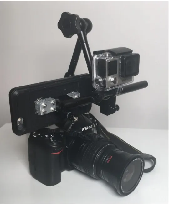
8. Camera capture rig. . . 29

9. Camera color and white balance calibration card. . . 30

10. Test environment with origin point. . . 31

11. Camera reference frame. . . 32

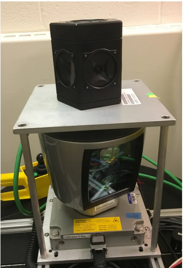
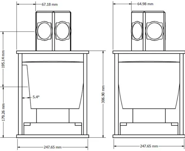
12. Camera and LIDAR mounted together. . . 33

13. Camera and LIDAR platform on motorized ground vehicle. . . 34

14. Translational offset between the LIDAR and the camera. . . 36

15. Calibration object used for finding relative rotation offsets. . . 37

16. Calibration object in each camera sensor. . . 38

17. Rotational offset between the LIDAR frame and the s1 frame. . . 38

18. Checkerboard for determining intrinsic camera parameters. . . 40

19. Subset of calibration images. . . 41

(13)

Figure Page 21. ArUco marker number 1, 6x6. . . 43 22. Test setup for capturing images of ArUco markers at

different distances. . . 44 23. ArUco marker placed at camera height. . . 47 24. Test environment, with landmark feature locations. . . 48 25. Training data used to model the area-distance

relationship for an 82mm×82mm marker. . . 53 26. Curve fitting results with rational model for an

82mm×82mm marker. . . 54 27. Marker distance for 82mm marker . . . 55 28. Distance error as a function of marker distance for

82mm×82mm marker. . . 55 29. Histogram and corresponding PDF when using the

82mm×82mm marker estimation function. . . 56 30. Training data used to model the area-distance

relationship for an 55mm×55mm marker. . . 57 31. Curve fitting results with rational model for an

55mm×55mm marker. . . 59 32. Marker distance for 55mm marker . . . 60 33. Distance error as a function of marker distance for

55mm×55mm marker. . . 60 34. Histogram and corresponding PDF when using the

55mm×55mm marker estimation function. . . 61 35. ArUco marker placement in the environment (left), and

marker as viewed from s1 (right). . . 62

36. LIDAR and camera frame synchronization. . . 63 37. ArUco keyframe selection . . . 64 38. Output of the keyframe calculation function for all

(14)

Figure Page

39. Output of the keyframe calculation function for marker 1. . . 66

40. Estimated distance to each marker for each keyframe. . . 66

41. Plot of platform odometry in GTSAM without covariance. . . 68

42. Plot of platform odometry in GTSAM with noise model properly tuned. . . 69

43. Initialization of landmark factors in GTSAM. . . 70

44. GTSAM factorgraph after Levenberg-Marquardt optimization. . . 71

45. Landmark location and marginal before (solid line) and after optimization (dashed line). . . 72

46. Pose uncertainty decreases when passing a landmark. . . 73

47. Position and orientation ofs1 for frame 3189. . . 74

48. General path taken to capture mobile camera imagery. . . 75

49. Images captured from the DSLR (top), iPhone (middle), and GoPro (bottom). . . 76

50. Cameras0 image with SIFT algorithm features shown. . . 78

51. Cameras0 image with SIFT algorithm features shown. . . 79

52. Cameras0 image with ORB algorithm features shown. . . 80

53. Rectified image from mobile camera, used to test image matching and pose recovery. . . 81

54. Detected SIFT features in the test image. . . 81

55. Detected SURF features in the test image. . . 82

56. Detected ORB features in the test image. . . 82

57. Top three image matches returned by computer. . . 83

58. SIFT features matched between images. . . 84

(15)

Figure Page 60. ORB features matched between images. . . 85 61. Pose recovery . . . 86

(16)

List of Tables

Table Page

1. Epipolar geometry variables. . . 16

2. GTSAM example factorgraph variable definitions. . . 21

3. GTSAM odometry factor parameters. . . 22

4. GTSAM bearing-range factor parameters. . . 22

5. Velodyne HDL-64E S2 Specifications. . . 26

6. FLIR Ladybug3 1394b Specifications. . . 28

7. Bearing offsets between the spherical camera and LIDAR. . . 35

8. Matlab calibration matrix variable definitions. . . 39

9. Marker distance and area used to create a distance estimation model for a 82mm×82mm marker. . . 52

10. Goodness of fit for different curve models based on RMSE of the 82mm×82mm marker data. . . 54

11. Marker distance and area used to create a distance estimation model for a 55mm×55mm marker. . . 58

12. Goodness of fit for different curve models based on RMSE of the 55mm×55mm marker data. . . 58

(17)

I. Introduction

1.1 Background

There is a need for a robust, easy to use indoor truthing system based on cam-era pose estimation. This truthing system would enable new advances in indoor and alternative navigation. Alternative navigation methods have been a subject of signif-icant research in recent years. These methods attempt to augment or replace systems that rely on the Global Positioning System (GPS) and other satellite-based methods for navigation. This is especially important for indoor environments, where satellite signals are occluded by building infrastructure.

This thesis, along with the corresponding research at the Air Force Institute of Technology (AFIT) Autonomy and Navigation Technology (ANT) Center, attempts to develop a 6 Degree of Freedom (DOF) indoor navigation system for low Size, Weight, Power and Cost (SWAP-C) cameras that fulfills several key requirements:

1. There is no permanent infrastructure required to implement the system. 2. Localization and navigation must be performed without GPS.

3. The method must be sensor-agnostic, compatible with different camera types, brands, and characteristics.

The foundation of this method is an accurate map created by a robot, using a high SWAP-C camera and Light Detection and Ranging (LIDAR) Simultaneous

(18)

Localization and Mapping (SLAM). This map, which is difficult to make indoors, is then used to determine the position and orientation of many types of low cost cameras.

1.2 Problem Statement

This research answers several problems. First, can image features of known di-mensions yield repeatably accurate range information using only monocular imagery? Next, can the relative poses of cameras with very different intrinsic characteristics be determined? Finally, can the true position and orientation of a camera in an envi-ronment be calculated within a reasonable amount of uncertainty?

1.3 Research Goals

The goal of this research is to recover the pose of a mobile camera within the environment, given an accurate map. The research attempts to collect monocular imagery data, establish a method of extracting bearing and range measurements from the data, and assesses the method’s accuracy. It also uses the measurements to create a map using a SLAM solution. After data analysis, the thesis proposes methods for improving and refining the truthing process.

1.4 Contributions

This research contributes to the fields of mapping, navigation, and computer vision in these specific areas:

1. Monocular ranging. This research proposes a method for extracting range

(19)

2. Method validation. This research quantifies the accuracy of the distance estimation method using real world measurements.

3. SLAM framework. A SLAM optimization framework with specific factors

and initial conditions is developed.

4. Indoor navigation. This research demonstrates an easily scalable navigation

method.

5. Computer vision feature algorithm evaluation. This work compares and

validates the use of different feature detection and matching algorithms to find the optimal setup for indoor navigation.

1.5 Thesis Overview

Chapter 2 contains the basic concepts and principles necessary to understand the thesis, including terminology and processes used for camera calibration, localization, and mapping. Chapter 2 also provides a review of previous work on robotic mapping and optical feature matching algorithms. Chapter 3 explains the specific equipment and SLAM factors used for the experiment. It also outlines the experiment method-ology for this research; including the range extraction algorithm, data collection, pose optimization, feature detection and matching, and pose recovery.

Chapter 4 discusses and analyzes the results from the experiments in Chapter 3. It compares different feature matching algorithms and evaluates the different models for estimating range from feature size. Chapter 5 concludes this research by giving an overview of results and conclusions. It also outlines future work, including proposed equipment and methodology changes, that will develop and broaden the results of this research.

(20)

II. Background and Related Research

This chapter is divided into two parts. The first part is a study of relevant and related research. Next, there is a detailed explanation of the underlying principles and concepts used throughout the thesis, including SLAM, data collection, optical feature descriptors, computer vision libraries, camera characteristics, and sensor syn-chronization.

2.1 Relevant Research

Although the concept of using SLAM to determine localization using on-board sensors in unknown environments is already a proven concept, the mapping results from SLAM systems are not used often to enable localization with only optical sensors. It is common to use many different sensors and systems to perform SLAM. These sensor types include

1. Inertial Measurement Units (IMU) [10] 2. Wheel odometry [55]

3. Sound Navigation and Ranging (SONAR) [9] 4. Computer vision with stereo cameras [26] 5. LIDAR [1]

Bogoslavskyi, in [6] and [13], proposed new methods for improving the quality of matching consecutive LIDAR scans. Additionally, [41], and [51] have demonstrated the benefits of SLAM systems for robot localization.

Multiple methods of performing SLAM have been studied, including methods based on Extended Kalman Filters (EKF) [3, 42], Extended Information Filter (EIF)

(21)

SLAM [53], FastSLAM [34], grid-based SLAM [18], and graph-based SLAM [17]. Thrun, Montemerlo, and Stachniss have provided research papers on these SLAM techniques. In [33], Thrun presents a new method of SLAM, featuring a factoring algorithm to efficiently represent features. This factor graph approach is gaining popularity because the algorithm’s complexity, compared to the Kalman-filter based approach, is reduced from O(K2) to O(M logK) time, where M is the number of particles, K is the number of features, and O is the algorithmic complexity.

2.2 Simultaneous Localization and Mapping

SLAM is a method for solving the localization paradox. If a position and orien-tation are precisely known, then generating a map of the local environment becomes trivial. Conversely, position and orientation can be determined quickly if the map is given. This interdependency can be circumvented by solving position updates con-currently with map updates, which is the foundation of SLAM. The idea of SLAM originated with Moravec and Elfes [40]. Smith, Self, and Cheeseman [49] improved the grid-based approach, while Durrant-Whyte and Leonard developed the feature-based SLAM method in [27].

SLAM can be separated into two sections. First, the “front end” comprised of the sensor data, landmark and environment information, and data association. The second section, or “back end”, is where the information is processed into a optimal SLAM solution. Different front ends and back ends can be combined depending on the specific needs.

The SLAM acronym was first coined in a mobile robotics survey paper presented at the 1995 International Symposium on Robotics Research [15], where the mapping and localization problems were combined into a single estimation problem. The SLAM problem is a critical part of autonomous navigation. SLAM posits that it is possible

(22)

for a mobile robot to build up a map of an unknown environment while simultaneously determining its location within the map, with an unknown location in an unknown environment. Durrant-Whyte and Bailey’s two tutorial papers on SLAM [54, 2] cover the basic principles and algorithms of SLAM in detail.

One key part of the algorithm development was the importance of the correlations between landmarks. The SLAM solution improves when the correlations between landmarks are stronger. Csorba developed much of the initial proof and theory of SLAM algorithm convergence in [11] and [12].

2.3 Iterative Closest Point (ICP) Matching

ICP is a method of matching two sets of corresponding point-clouds. The main goal of ICP is to determine a translation and rotation that minimize the sum of the squared error between corresponding point locations. The critical assumption behind ICP is that the correct correspondences are known. Without correct correspondences, the algorithm may terminate at a local minimum. If data association is an issue, having an accurate guess of rotation and translation can make the local minimum align with the global minimum.

ICP can trace its origins to the 2D template matching with the Singular Value Decomposition [56]. This method used a tiered approach, where a coarse registration reduced the computational intensity of the final cross-correlation calculation. The full ICP algorithm was applied to matching 3D shapes, curves, and surfaces in [5], and expanded to free-form shapes in [57]. A 2D example of ICP is shown in Figure 1. In the example, a set of points is chosen from each line. One of the point sets is iteratively moved and transformed to minimize the distance between each point set. Note that any inaccuracy in points chosen degrades the quality of the match.

(23)

LIDAR Scanners.

Laser scanners are a popular method for generating point clouds for SLAM, using either phase-shift or time of flight (TOF) methods. Measuring the doppler shift has the added benefit of providing the velocity of the reflecting surface along with the distance. TOF systems offer simplicity, measuring the time a laser pulse takes to travel to and from a surface. The travel time can be quickly converted to a distance using the equation:

d = 1

2ct (1)

where d is the distance, c is the speed of light, and t is the travel time of the laser pulse. Laser scanners have fast and accurate measurements compared to other sensors, each measurement only takes microseconds with an angular resolution of less than 0.5◦. Angular resolution can be a disadvantage in feature-dense environments, since the laser pulse may not detect every object. Additionally, materials such as glass or water can have poor data returns. Sonar, which was originally an acronym for SOund Navigation And Ranging (SONAR), uses sound wave TOF in a method similar to the laser scanner.

A new method of ICP, proposed in [20], accounts for the local minimum trap by searching the point cloud data for corresponding features. These geometric fea-tures can be anything; including curvature, surface normal vectors, and point cloud density. The results demonstrated that the augmented ICP algorithm improves the convergence speed and the convergence interval, even without setting a proper initial estimate.

(24)

Figure 1: Illustration of the iterative closest point method to align two lines [48].

Additional SLAM Methods.

Since the introduction of SLAM in 1995, many different methods have been in-troduced. Some common types include Extended Kalman Filter (EKF) SLAM [50], FastSLAM 1 [34], FastSLAM 2 [32], Occupancy Grid SLAM [35], Oriented FAST and Rotated BRIEF (ORB) SLAM (ORB-SLAM) [37], and incremental Smoothing And Mapping (iSAM) [23].

EKF SLAM models a map of sensor and landmark states using a Gaussian vari-able. The two stages of EKF, prediction and correction, process the map. The prediction stage propagates the Gaussian variable through the filter to estimate the map at the next stage. The correction stage brings in sensor data to improve the SLAM solution. EKF SLAM is causal, but a forward-backward smoother can be added to improve the solution even further. Sol`a, in [50], presents a good tutorial of EKF SLAM including practical examples.

(25)

FastSLAM 1 and FastSLAM 2 were first introduced by [34] and [32], respectively. They have quickly overtaken EKF SLAM in popularity. While very similar to EKF SLAM, FastSLAM 1 substitutes a Rao-Blackwellised particle filter for the EKF. Fast-SLAM 2 improves the Fast-SLAM solution by using a different proposal distribution than the original FastSLAM algorithm. These algorithms converge well for linear problems, but have difficulty representing highly non-linear systems [3].

Occupancy Grid SLAM reduces the impact of data-disassociation by representing the environment as a block of cells. As the sensors traverse the environment, sensor data is used to determine the probability that a cell is empty or full. These probability maps, called occupancy grid maps, were introduced to SLAM in [35]. Millstein’s research in [31] demonstrates a thorough application of Occupancy Grid SLAM.

ORB-SLAM, introduced in 2015 [37], is a camera-based SLAM approach that uses image features for every aspect of SLAM, from mapping and localization to handling loop closures. ORB-SLAM has several advantages besides using one sensor for the entire system. It operates in real time, in a wide range of environments and scales, and only increases in size if the camera environment changes.

The iSAM method was introduced in 2008 [23] as an exact and efficient SLAM solution. It is very good for non-linear systems since all previous poses are kept as part of the estimation stage. The four characteristics that are met by iSAM are:

1. Exactness: no approximations can be made, even with nonlinear measurements. 2. Efficiency: data processing speed must be adequate for real-time use

3. Data associations: information for data association must be readily available. 4. Applicability: iSAM must be able to solve a wide range of problems on many

(26)

The effiency in iSAM is possible by only re-factoring when a large change is present, instead of every time a measurement is made.

Georgia Tech Smoothing And Mapping (GTSAM) toolbox.

GTSAM is based The GTSAM toolbox was developed at the Georgia Institute of Technology by Dellaert along with many of his students and collaborators [14]. GTSAM is a C++ library for solving factor-graph based problems. In addition to modeling and solving SLAM problems, it can also solve Structure From Motion (SFM) problems and more complex estimation problems. Along with the C++ library, GT-SAM also provides a MATLAB interface, used extensively for this research, which allows for algorithm development, modeling, visualization, and user interaction.

Factor graphs are bipartite graphs with two components, factors and variables. Factors represent probabilistic information, derived from measurements or prior knowl-edge. Variables represent random variables. Koller and Friedman provide tutorials on factor graphs, along with other graph-based models including Bayes networks, in [24]. Georgia Tech has been making many strides in navigation and mapping, including SLAM with 3D and 2D Sensors [52] and analyzing the impact of sensor precision on SLAM accuracy [44].

Levenberg-Marquardt Optimization.

The Levenberg-Marquardt (LM) optimization algorithm has become a standard method for solving non-linear least-squares problems. It is based on the work of Levenberg [28] and Marquardt [30]. It is an iterative technique that locates the minimum of a multivariate function that is expressed as the sum of squares of non-linear real-valued functions. The LM algorithm can be considered as a combination of the gradient descent method and the Gauss-Newton method. If the multivariate

(27)

function is far from the optimal solution, the algorithm approximates the gradient descent algorithm. If the function is close to optimal, it approximates the Gauss-Newton method. The algorithm’s implementation and theory are described in detail in [36].

2.4 Data Collection Methods

Different SLAM algorithms and methods can utilize a wide range of sensors. The most common type are exteroceptive sensors including laser scanners, sonar, and cameras. Combinations of these sensors are often used, or paired with interoceptive sensors such as wheel encoders or inertial sensors. These sensors only measure posi-tion indirectly, using velocity and acceleraposi-tion, they do not interact with the external environment. Exteroceptive sensors, while expensive compared with wheel odometry and commercially-available inertial sensors, offer more accurate long-term measure-ments. Often, both types of sensors are used together because of their complimentary characteristics.

SLAM relies on an estimate of motion between successive poses, often referred to as odometry. This motion is measured using the sensors above. Odometry from wheel encoders measures the rotation of each wheel, using the wheel radius and rotation to determine the vehicle’s motion. Inertial sensors include accelerometers and gyrometers, which measure linear and angular acceleration. These sensors drift significantly in the long-term, making them insufficient for SLAM by themselves. However, they are very stable in the short-term, smoothing the jitter inherent to many exteroceptive sensors.

(28)

2.5 Optical Feature Descriptors

Optical feature descriptors are features that can be repeatably found in images of a specific scene. These features can be identified even after changes in rotation, scale, and lighting conditions. Many different algorithms have been developed, each with their own benefits and problems. This section details the specific algorithms used for this research along with the specific toolbox used to apply the detectors to each image.

SIFT.

The Scale Invariant Feature Transform (SIFT) was developed by D. G. Lowe in 2004 [29], it has since become a widely-used feature detection and description algorithm. The SIFT detector uses an approximation of a Laplacian-of-Gaussian (LoG) operator, called a Difference-of-Gaussians (DoG) operator: Feature-points are detected by searching local maxima using DoG at various scales of the subject images. A 1616 pixel box around each detected feature is then further analyzed and broken into sub-sections or blocks, rendering a total of 128 bin values. SIFT is computationally intensive, but is highly invariant to rotations, scale, and affine changes.

SURF.

The Speeded Up Robust Features (SURF) detector was introduced in 2008 [4]. it relies on a tiered Gaussian analysis of images and the determinant of a Hessian Matrix. Feature detection speed is improved by using only using 64 bins. The main advantage of SURF over SIFT is its lower computational cost. While SURF features are also invariant to rotation and scale, they are not as invariant to affine changes. The descriptor can be extended to 128 bin values to cope with affine variance at the cost of computation time.

(29)

ORB.

ORB, was developed by E. Rublee et al. in 2011 [46]. It is a combination of two modified feature detection algorithms: Features from Accelerated Segment Test (FAST) [45] for the feature detection, and Binary Robust Independent Elementary Features (BRIEF) [8] for the feature description. FAST corners are detected at vary-ing scales, then the detected corners are processed with a Harris Corner Detector to select the most optimal points. The original BRIEF description method is unstable with respect to rotation, so modification is required to make ORB features rotation invariant. ORB features are also invariant to scale and some affine changes.

2.6 Open Source Computer Vision Library (OpenCV)

OpenCV is an open source computer vision and machine learning software library

1_{. It provides a framework for designing and testing multiple computer vision}

appli-cations. OpenCV is a Berkley Software Distribution (BSD)-licensed library, which makes it popular for academic and commercial settings alike. The library has been downloaded over 14 million times, with an estimated 50 thousand users. This popu-larity has built a large community of users and collaborators, and grown to include over 2500 algorithms for computer vision and machine learning [7]. OpenCV Forums are a resource for tutorials, operating instructions, and instructional manuals. Along with the OpenCV Forums, [22] was used extensively to accomplish this research.

OpenCV supports Windows, Linux, Android and Mac OS operating systems. It is written natively in C++, but it also integrates with Python, Java, and MAT-LAB. OpenCV algorithms will be used specifically for image calibration and feature matching in this thesis.

(30)

2.7 Camera Characteristics

Camera models are used to describe the relationship between information from the picture, on the image plane, and the actual world. The models enable comparisons between different cameras. The camera model used for this research is the pinhole camera model, which is widely used.

Pinhole Camera Model.

The most simplistic model of a camera is the Pinhole Camera model. A pinhole camera has a single small aperture (a pinhole) and no lens. Light passes through the aperture and projects an inverted image on the rear of the camera, or image plane. The distance from the aperture to the rear of the camera is known as the focal length. There is also a virtual image plane, one focal length in front of the aperture, which contains the non-inverted image. Many cameras can be fully described by using a pinhole camera along with additional intrinsic and extrinsic parameters. These additional parameters, introduced in [21], vary from sensor to sensor.

Extrinsic Parameters.

Extrinsic parameters describe the position and orientation of the camera. This can either be the relative to an origin point and axis in the environment, or relative to a second camera or image. External parameters change whenever a camera is moved or re-oriented. The extrinsic parameters transform world feature points into camera coordinates, and from camera coordinates into world feature points.

Intrinsic Parameters and Calibration.

Intrinsic Parameters transform camera coordinates into the image plane. Some of the parameters included are focal length, radial lens distortion, tangential lens

(31)

distor-tion, and sensor skew. Because these parameters are different for each camera, image matching algorithms require a calibration step to account for the camera differences. Images from a camera can be rectified using the camera calibration parameters. Rec-tifying an image corrects for the different types of distortion. There are two prominent methods of calibration. The first, known as self-calibration or auto-calibration, takes non-calibrated images from multiple views of an object to calculate the calibration matrix [19].

The second method is a batch approach which uses at least 10 images of a planer pattern with measured feature sizes, for instance a chess board. This method is more accurate and more common than self-calibration. First, specific points or corners are identified, Then the coordinates in real-world space and the coordinates in each image are used to solve for the distortion coefficients. Because of the method’s popularity there are many applications and tutorials detailing its procedures. Lambers presents a calibration approach using OpenCV [25].

2.8 Multiple-Camera Registration

Images of unique features taken from multiple cameras can be used to determine the extrinsic parameters of the cameras. That is, the rotation and translation that separate the sensor coordinate frames. This process works through the use of epipolar geometry, shown in Figure 2. The variables used, listed in Table 1, are as follows: Point q is an optical feature that appears in both cameras. O1 and O2 are the

camera’s optical centers, separated by some baseline. The epipolar plane is the plane that contains the points q, O1, and O2. The lines l1 and l2 are where the epipoplar

plane intersects each image plane. Each camera also has an epipole, or the point where the baseline intersects the image plane. These epipoles are e1 ande2 for sensor

(32)

andp2. This works well for applications such as stereo-vision navigation and ranging,

when the baseline is either fixed or measurable.

Figure 2: Epipolar geometry.

Table 1: Epipolar geometry variables.

Variable Definition

q optical feature point

O1 camera 1 optical center O2 camera 2 optical center

l1 intersection of epipolar plane and image plane 1 l2 intersection of epipolar plane and image plane 2 e1 camera 1 epipole

e2 camera 2 epipole

p1 q projected onto image plane 1 p2 q projected onto image plane 2

Essential and Fundamental Matrices.

Epipolar geometry can be expressed in camera coordinates using the Essential matrix E, a 3×3 matrix that only depends on the extrinsic parameters R and T.

(33)

The Essential matrix consists of five parameters (three rotation parameters and two translation parameters). It has two constraints:

1. the determinant is zero.

2. the two non-zero singular values are equal.

E=R       0 −Tz Ty Tz 0 −Tx −Ty Tx 0       (2)

Epipolar geometry can also be can be expressed in image coordinates by using the Fundamental matrixF, which depends on the extrinsic and the intrinsic parameters. The Fundamental matrix always has a rank of two, and contains seven parameters (two for each of the epipoles and three for the homography between the two epipolar lines). If the cameras are calibrated, then the point location from each sensor is given with respect to its camera’s coordinate frame and the Essential matrix can be used. The Fundamental matrix can be used with uncalibrated cameras.

To recover a relative pose between two cameras, the Essential matrix must be de-rived from sets of corresponding points in images from two calibrated cameras. Using the Essential matrix and the pose estimation algorithm, introduced by David Nist´er in 2004 [39], the relativeRand Tmatrices can be recovered. Although Nist´er’s algo-rithm only requires five data points to be tractable and convergent, it often requires many more to account for noise and co-planar features [43].

(34)

2.9 Sensor Synchronization

When using multiple sensors, it is necessary to synchronize the data between sensors. To minimize timing errors, the signals can be triggered by a single signal, or synchronized using frames with feature common to all sensors. This thesis uses the frame synchronization method which, while less accurate than using single timing sources, is much simpler to implement.

Frame Synchronization.

When using frame synchronization, timing differences between sensors are calcu-lated by interpolating between sets of data. This is done by identifying a temporal feature at the start and end of each data set. It can be as simple as observing the start and end of movement, or using specific movements at determined frequencies. This method is practical for short tests with a limited number of sensors and if a timing error of _{f ramerate}1 is acceptable.

External Timing.

External timing sources can trigger data collection on most sensors. They can run on their own internal frequency generator, or be synchronized to a global reference such as GPS time if required. Sensors can have very different signal requirements, ranging from a single low-voltage pulse to an Ethernet data packet, oftentimes through a dedicated synchronization port. Depending on the type of signal and the accuracy of the timing circuit, synchronization within 10 ns is possible.

(35)

III. Methodology

3.1 Objective

The purpose of this research is to test the efficacy of using LIDAR and camera sensors to generate a reference database of images (taken from SLAM-derived posi-tions) and use that database to determine the location and orientation of a new image. The experiment execution necessitates the use of multiple sensors, so calibration and image rectification will be used to properly characterize the sensor-to-sensor relation-ships and sensor-to-feature relationrelation-ships. The specific experiments aim to accomplish several goals:

1. Measure the accuracy of calculating range data from an image with known feature sizes.

2. Generate a set of geo-referenced images using SLAM techniques.

3. Collect sets of images using the same environment as the SLAM dataset. 4. Solve for the 3D position and orientation of an camera using the SLAM dataset.

This chapter begins with the setup and factors used by GTSAM. Then an overview of the important markers, equipment, and sensors used in the experiments. Next, there is a description of the different coordinate systems and frames, followed by the physical relationships between sensor frames. Finally, there are overviews of each experiment.

3.2 GTSAM Setup

This thesis uses a 2D landmark-based SLAM problem, with prior factors, odom-etry factors, and landmark measurement factors. Figure 3 is an example of a factor

(36)

graph for a landmark-based SLAM problem. The variables are listed in Table 2. There is one landmark l1, along with three pose variables: x1, x2, and xn,

represent-ing the poses of the platform over time. As shown in the example, there is a factor

p on the pose x1 that encodes prior knowledge about x1, two factors that relate

suc-cessive poses: o1 and o2, and two factors that relate poses to the landmark: br1 and br2.

Figure 3: Example factorgraph with pose and landmark factors.

Prior Factors.

Prior factors are unary factors that encode the prior knowledge of each pose or landmark. They describe a probability of an initial condition. In this thesis, there is a prior factor based on the approximate starting location of the platform, as well as the approximate locations for each of the landmark features. These are passed to GTSAM as PriorFactorPose2 functions. The PriorFactorPose2 function requires certain parameters, including the pose or landmark ID and the position constraint.

(37)

Table 2: GTSAM example factorgraph variable definitions.

Variable Factor Used Definition

p PriorFactorPose2 prior factor

x1 - 1st pose

x2 - 2nd pose

xn - nth pose

l1 - landmark

o1 BetweenFactorPose2 odometry factor from x1 tox2

o2 BetweenFactorPose2 odometry factors from x2 toxn

br1 BearingRangeFactor2D factor from x1 tol1

br2 BearingRangeFactor2D factor from xn to l1

Each prior factor also has an associated noise model which can account for measure-ment uncertainty. This is an Example of a prior factor in MATLAB that adds a prior from pose 1 to the origin:

PriorFactorPose2(x1, Pose2(0, 0, 0), noiseModel.Diagonal.Sigmas([1; 1; 0.1]));

Odometry Factors.

Odometry factors are binary factors that relate two poses. This is expressed in GTSAM by theBetweenFactorPose2 function, which is expressed in MATLAB using the command:

BetweenFactorPose2(x1, x2, odometry, noise))

The function input parameters are described in detail in Table 3. This thesis only uses the odometry factors to relate consecutive platform poses. For example: pose 1 to pose 2, pose 2 to pose 3, pose n-1 to pose n. The parameters required for an odometry factor are shown in Table 3.

(38)

Table 3: GTSAM odometry factor parameters.

Parameter Definition

x1 1st _{pose ID}

x2 2nd pose ID

odometry relative translation and rotation from the 1st _{pose ID to the 2}nd _{pose ID}

noise diagonal Gaussian noise model for the x position, y-position, and orientation

Bearing-Range Factors.

Binary factors can also be used to relate a pose and a landmark. This uses a dif-ferent GTSAM function, theBearingRangeFactor2Dfunction, which uses the relative bearing and range from a pose to a specific landmark. Ensuring that measurements are associated with the correct landmark is crucial to SLAM. Incorrect matches be-tween measurements and landmarks can have a detrimental impact on the SLAM result. This research simplifies the data association problem by using the ArUco marker ID to assign a unique identifier to each landmark.

This function is expressed in MATLAB using the command:

BearingRangeFactor2D(x1, l1, Rot2(angle), range, noise)

each parameter is described in detail in Table 4.

Table 4: GTSAM bearing-range factor parameters.

Parameter Definition

x1 Pose ID

l1 Landmark ID

Rot2(angle) Relative bearing to landmark range Range to landmark

(39)

Optimizer.

The GTSAM factors and variables, in a factor graph structure, are compiled into a an optimizer along with any initial conditions. Because the odometry factors involve the orientation and movement of the platform, which are not linear, the optimizer also needs to be non-linear. The optimizer class linearizes the factor graph multiple times to minimize the non-linear squared error specified by the factors. The Levenberg-Marquardt algorithm, described in detail in Subsection 2.3, is a good choice because it often converges, even if it starts very far off the final minimum. The MATLAB command for the Levenberg-Marquardt optimizer is:

LevenbergMarquardtOptimizer(graph, initial);

3.3 Equipment and Sensors

ArUco Markers.

Because loop closures and revisits are such a critical part of SLAM, there is a need to create unambiguous data associations between multiple views of a single feature. The features in this case are ArUco markers, which have unique IDs that can be detected and processed using OpenCV. ArUco markers are available in a wide range of libraries, depending on how many unique features are available and how many bits each marker has. For this thesis, the 6x6 library of 250 unique markers provides enough unique IDs without having a higher bit density. Only the first 25 6x6 markers, shown in Figure 4, are used. Each marker was printed at a scale of 82 mm by 82 mm with the unique ID below each marker, as shown in Figure 5, since the markers are not human-readable.

(40)

(41)

(42)

Velodyne HDL-64E S2 LIDAR.

The LIDAR used for the experiments is the HDL-64E, version S2, from Velodyne. The HDL-64E has 64 lasers, mounted in pairs of 32 lasers on upper and lower blocks. Both blocks are mounted onto a rotating platform, spinning at 600 rotations per minute. This design provides a much richer point cloud than previous designs in which a singe laser is fired through a rotating mirror. The HDL-64E has the specifications listed in Table 5. Several methods have been studied for improving the accuracy of the HDL-64E [16]. Velodyne also provides software for viewing, calibrating, and parsing the raw LIDAR data into other formats. An example of the velodyne viewer is shown in Figure 6, compared to the MATLAB point cloud viewer in Figure 7.

Table 5: Velodyne HDL-64E S2 Specifications.

Parameter Value Unit Spin Rate 300-1200 RPM Vertical Field Of View 26.8 degrees Horizontal Field Of View 360 degrees

Sensing Range 120 m Range Accuracy 15 mm Output Capture Format PCAP

-FLIR Ladybug3 1394b Spherical Camera.

The camera used to capture the geo-located images is the FLIR Ladybug3 camera. It is a comination of six 2 MP sensors with global shutters that enable the system to collect video from more than 80% of a full sphere. The data from each camera is col-lected and transmitted over an IEEE-1394b (FireWire) interface. JPEG-compressed 12MP resolution images can be captured up to 15fps. The Ladybug3 was designed for weather-resistant high-resolution, direct FireWire, and synchronized image capture. These specifications are listed in Table 6.

(43)

Figure 6: Velodyne point cloud viewer.

(44)

Table 6: FLIR Ladybug3 1394b Specifications.

Parameter Value Unit Spherical Coverage 80 percent

Resolution 2 MP Frame Rate 15 fps

Interface IEEE-1394b -Output Capture Format JPEG

-Mobile Cameras.

To collect the images that compare against the geo-referenced image set, three mobile cameras are used. These are a Digital Single Lens Reflex (DSLR) camera, a mobile phone camera, and a high-speed action camera. This combination represents a wide range of sensors. The DSLR used is a Nikon D7000 with a wide angle lens, collecting 2.074 MP at 30fps. The mobile phone sensor is an Apple iPhone 6s, collect-ing 2.074 MP at 60fps. Finally, the action camera is a GoPro Hero4 Silver collectcollect-ing 2.074 MP at 60fps.

All three cameras are connected together using the camera rig shown in Figure 8. Recording is started for the cameras and the rig is pointed at the color calibration card in Figure 9, which is used as a reference for white balance and color correction. Finally, the rig is moved through the hallways, following the path travelled by the geo-referenced camera at a maintained height of approximately 1.5 meters. The rig is oriented straight ahead for one pass, 45◦ right for one pass, 45◦ left for one pass, and straight ahead for the final pass.

3.4 Coordinate Systems and Reference Frames

The experiments conducted in this research require cooperation between several different sensors and environments, which have their own unique frames of reference.

(45)

(46)

Figure 9: Camera color and white balance calibration card.

These different reference frames, such as the environment frame, the mobile camera frame, and the platform frame, encompassing the LIDAR frame and the spherical camera frame. Although there is also some global reference frame, it is unused since every sensor can be related to a common local environment. The environment cov-ers the area of AFIT in which the experiments are conducted. The environment is mapped by overlaying a 3-dimensional right-handed Cartesian coordinate system onto the hallways where the positive x-axis is West, the positive y-axis is South, and the positive z-axis is up. This orientation is shown along with the test environment in Figure 10.

The mobile camera frame follows common convention as shown in Figure 11, where the sensor lays on thex-y plane and thez-axis is out the front of the camera. This is the same for all three cameras. The frame of the motorized platform that houses the LIDAR and the camera is simplified by sharing a common origin, namely the center

(47)

Figure 10: Test environment with origin point.

of the LIDAR sensor. Thex-axis is oriented in front of the platform, they-axis to the left, and the z-axis up. The raw LIDAR data is given with the y-axis out the front of the sensor, the x-axis to the right, and the z-axis up. The LIDAR can therefore be related to the platform by a yaw of 90◦, or by the DCM:

Rplatf orm_LIDAR =

      0 1 0 −1 0 0 0 0 1       (3)

Applying this DCM to the LIDAR data orients both frames, making the primary motion of the platform and the LIDAR fall along the x-axis.

The spherical camera is rigidly affixed to the platform. Since the panoramic image is comprised of six individual sensors, each sensor has its own coordinate frame, following the convention used on the mobile cameras above. These sensors will be

(48)

denoted as s0 through s5, and their rotational offsets from the LIDAR frame will be

discussed in Subsection 3.5.

Figure 11: Camera reference frame.

The camera and LIDAR are both attached to an aluminum platform, shown in Figure 12, so the offsets remain constant throughout the experiment. To maintain a constant height, the platform traverses the environment on a motorized ground vehicle. The vehicle carries the power supply and data recorder for the sensors. This vehicle is shown with the platform attached in Figure 13.

3.5 Physical Characterization

The first step of each experiment is to determine the physical characteristics of the system, namely the translation and rotation from one frame of reference to another. To generate a set of geo-referenced images using SLAM, the corresponding relation-ships between LIDAR, camera, and landmark features must be well-understood. Ad-ditionally, the intrinsic parameters of each camera must be determined to account for effects such as focal length and lens distortion.

(49)

(50)

(51)

LIDAR to Camera.

Determining the relationship between the LIDAR frame and the camera frame is a combination of physical measurements and data analysis. The relationship remains constant throughout the experiment because the LIDAR and the camera are rigidly affixed to the same structure, as shown in Figure 14. The translational offset between frame origins is calculated by the lateral, longitudinal, and vertical distance between the sensor origins.

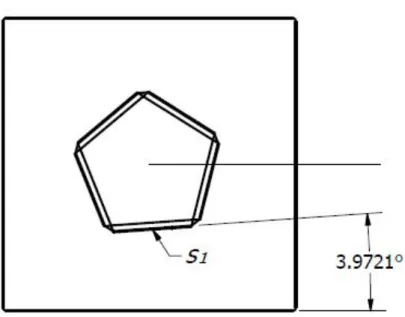
Calculating the rotational offset between sensors requires identifying a feature in both sensor data sets. This is accomplished by finding an object in an image that is separate from any background objects.

The calibration rod can be seen in Figure 15. When the platform is rotated, it appears in each sensor frame as shown in Figure 16. The tall and thin rod has enough data to determine relative roll and yaw. Since the LIDAR and combined sensors both have 360 degree horizontal fields of view, relative pitch can be calculated by measuring the roll of the other image sensors. The resulting rotational offset for the sensor capturing landmark data is−86.0279◦, shown in Figure 17. Table 7 shows the offsets for each individual sensor.

Table 7: Bearing offsets between the spherical camera and LIDAR.

camera sensor cam-marker LIDAR-marker LIDAR-sensor 0 -0.110◦ -17.040◦ -16.93◦ 1 -3.123◦ -89.151◦ -86.0279◦ 2 -2.372◦ -165.350◦ -162.978◦ 3 -4.450◦ 117.432◦ 121.8812◦ 4 3.489◦ 59.928◦ 56.4392◦

(52)

(53)

(54)

Figure 16: Calibration object in each camera sensor.

(55)

Camera to Camera.

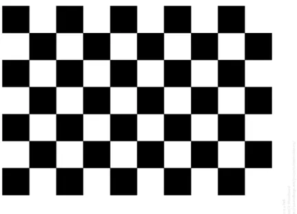
The intrinsic differences in cameras must be accounted for to properly determine the relative position of two or more cameras. The camera parameters for each camera are measured prior to each data collection using MATLAB’s camera calibration tool, along with at least 20 images of the calibration checkerboard shown in Figure 18. By importing images at different skew angles and positions, as in Figure 19, MATLAB returns the calibration matrix in Equation 4, with the variables in Table 8.

C=       F ∗sx 0 0 s F ∗sy 0 cx cy 1       (4)

Table 8: Matlab calibration matrix variable definitions.

Variable Definition

cx optical center x component

cy optical center y component

s skew parameter

F focal length in mm

sx number of pixels per world unit x

sy number of pixels per world unit y

For instance, the calibration of the mobile phone camera, shown in Figure 20, resulted in this intrinsic matrix:

C=       3486 0 0 3.3238 3501.7 0 1995.6 1528.2 1       (5)

(56)

Figure 18: Checkerboard for determining intrinsic camera parameters.

This calibration method is performed before each test and for each camera.

Experiment Overview.

The following sections detail the experiments and procedures used to enable the camera pose estimation. The first experiment explores the efficacy and accuracy of using monocular images to create range and bearing measurements. The second experiment uses vision and LIDAR SLAM, along with the bearing and range data from Experiment 1, to generate geo-referenced images. The third experiment creates a collection of test images from different cameras. The final experiment uses the findings from the first 3 experiments to determine the position and orientation of the mobile cameras.

3.6 Experiment 1 - Calculate Range Data from an Image

The objective of the experiment was to demonstrate that range can be calculated to a fair degree of accuracy based only on the relationship between the number of

(57)

Figure 19: Subset of calibration images.

(58)

pixels of a feature with a known feature size, and the feature’s distance from the sensor.

SLAM uses landmark measurements to improve the mapping solution. Since the spherical camera is already capturing data along with the LIDAR, it follows that images should be used to measure range and bearings to landmarks. While a single camera can easily tell the bearing to the landmark, that is insufficient for the SLAM algorithm. By using features of a known size, a range estimate can be calculated from a single camera. This experiment is designed to relate the distance of the camera to image features of known sizes, in this case ArUco markers.

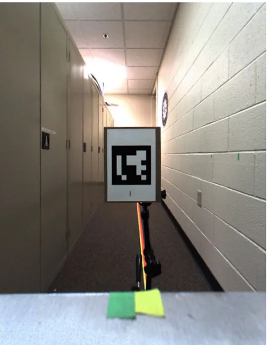
The objective of the experiment is to demonstrate that range can be calculated based on the relationship between feature size in pixels and feature distance. Images of the ArUco marker shown in Figure 21 are taken at a series of known distances at the same height as the camera, as shown in Figure 22. After being rectified, the images are processed to identify the marker in each image and calculate the marker corner locations. A short MATLAB script takes the corner locations and calculates the marker area. The MATLAB Curve Fitting Toolbox is used to process the data and create a model of the pixel-distance relationship. Root mean squared error is used to evaluate the goodness-of-fit for each curve fitting model, through which the rational model in Equation 6 provides the least error.

y= p1x+p2

x2₊_q

1x+q2

(6)

3.7 Experiment 2 - Generate a Set of Geo-Referenced Images

The first step for this experiment is to set up ArUco markers at known locations so thats1 of the spherical camera will pass directly in front of them. The bearing and

(59)

(60)

Figure 22: Test setup for capturing images of ArUco markers at different distances.

(61)

range factors to these landmarks will improve the end result of the factor graph opti-mization method. To simplify the bearing and elevation measurements, each feature is placed at a height of 0.934 m, the height of the camera, as shown in Figure 23. Ad-ditionally, each range measurement is only taken when the camera passes directly in front of the marker, limiting the bearing measurements to a 5◦ window. This method of sorting markers and identifying the most suitable measurements to use as bearing and range factors is listed in detail in Appendix A.

Once the markers are placed throughout the environment, their position must be recorded. First, the marker position in the environment frame is measured using a surveying tape. Next, the measurements are converted from the tape, with gradua-tions in ₁₀1 of a foot, into meters to correspond with the other distance measurements throughout the thesis. Finally, the marker positions are added to the environment map, as shown in Figure 24.

After the measurements are made, the LIDAR and camera are activated and the data capture programs begin recording. When the individual programs are operat-ing correctly, several correlation movements are performed by movoperat-ing the platform slightly. This makes it possible to temporally align the camera and LIDAR to within one frame. Then the platform is moved around the environment, moving camera s1

past the landmark features. This loop is traversed three times, stopping after a final pass of landmark 1 which acts as a loop closure for the final pass. Again, several movements are made with the platform to account for drift between the sensors. The data from both sensors is synchronized as described in subsection 2.9. The recti-fied images from s1 are passed through an ArUco marker detection algorithm which

returns the frame number, marker ID, and marker corner location in pixels. The algorithm detects many different images for each pass. However, only the picture when the marker is closest to the image center is used. This recreates the conditions

(62)

of Experiment 3.6, where the marker was centered in the image and only the range was changed, maximizing the range measurement accuracy.

The following process is used to find the optimal frame for each landmark pass, while still creating landmark measurements for successive passes. First, the center of the marker in each image is calculated using the corner locations, and the absolute distance from image center to marker center is passed into the function that deter-mines the key frames for each marker ID. Then the pixel area of each marker in a key frame is passed into the distance estimation model from subsection 3.6 to calculate the estimated range. Finally, the relevant information for creating bearing and range factors is compiled and stored.

The original LIDAR data is processed in several steps. First, running the propri-etary calibration program corrects for distortion and other factors that are inherent in the data. Then the points for each LIDAR frame are exported into MATLAB, where the frames are stored as point cloud objects. Performing ICP-based point cloud registration on consecutive frames determines a relative change in position and orientation which is used to generate odometry factors.

GTSAM is used to process all of the information into an optimal trajectory es-timate. The platform starting location and heading, along with all of the landmark positions, are added to the factor graph as constraints. These constraints have some prior noise model associated with them to allow for some adjustment during optimiza-tion. Next the odometry factors are added, consisting of the change in rotation and translation from ICP, a pose ID, and a noise model of the measurements. Then the bearing-range factors from the ArUco marker images are added, using the odometry pose that is closest to the image capture time. The noise models for the odometry and bearing-range factors are tunable parameters. In this case, the noise models are adjusted so that the position covariance for each pose and landmark encompasses the

(63)

true positions.

After GTSAM compiles the noise models and factors into a factor graph, it is optimized using a non-linear Levenberg-Marquardt optimization. Once the optimal pose locations and bearings are found, the extracted measurements are linked to each camera frame. Since the camera frame is not directly synchronized with odometry poses, the measurement is an interpolation of the two nearest pose measurements.

Figure 23: ArUco marker placed at camera height.

3.8 Experiment 3 - Collect Imagery in the Same Environment

To prove the concepts put forward in Section 1.2, there must be images to test. Three different cameras were used to take images to ensure that different cameras can still be localized. The image sets from the three cameras are collected simultaneously. First, all three cameras are calibrated using the method outlined in Subsection 3.5.

(64)

Figure 24: Test environment, with landmark feature locations.

3.9 Experiment 4 - Extract Relative Pose from Matched Images

The first part for this experiment is to build a database of image feature descriptors from the geo-referenced camera data. For this, the rectified images from s0 to s5

are passed through an OpenCV image processing algorithm to find all of the SIFT features. The SIFT feature descriptors for the different sensors are then compiled into a single list. This is repeated for each geo-referenced image frame. The feature lists, organized by image frame, are stored in a database.

Test images are selected from the mobile camera data, and processed using the same image feature algorithms. Then, the image features are compared to the feature database using RANSAC to determine if the mobile image has some overlap with a geo-referenced image. To reduce the possibility of having a false match, the three most likely matches are displayed to the user who can select a match that has two overlapping images.

After a matching image set is found, specific image features in both images are found and ranked based on likelihood. The essential matrix is calculated for both

(65)

images using the principles in Section 2.8. Next, the essential matrices are used to recover the relative R and T matrices, which describe the orientation of the mobile camera relative to spherical camera and the location of the mobile camera relative to spherical camera, respectively.

The pose recovery algorithm returns a translation in the form of a unit vector. To determine the actual translation, additional steps are required. First, the pose recovery calculation is repeated for the poses 15 frames before and after the selected pose. Next, the intersection of the three translation vectors is calculated. Each vector

v has an origin pointa and the intersection pointcis the closest point of intersection for all three vectors. The distance of this point to the line is:

H = k(c−a)×dk

kdk (7)

With the identity (a×b)·(a×b) =kak2_kbk2₋₍_a_·_b₎2 _{the distance of this point}

to the line becomes:

H2 = kc−ak

2_kdk2 _{− k}₍_c₋_a₎_·_dk2

kdk2 (8)

H2 =kc−ak2₋k(c−a)·dk2

kdk2 (9)

To find a csuch that the sum is minimized, the derivative with regard tocshould be zero: 0 = 3 X i=1 c−a(i)−d(i) (c−a(i))·d(i) kd(i)k2 (10) The final stage is to convert the mobile camera pose from the camera coordinate frame back to the local environment frame using the relative rotations and translations described in Section 3.4. The first step is to calculate the Direction Cosine Matrix

(66)

(DCM) Cfrom the mobile camera to the environment using Equation 11. R1 is the

DCM from the spherical camera to the environment, and R2 is the DCM from the

mobile camera to the corresponding spherical camera sensor. The camera position is calculated using Equation 12, where V is the position of the mobile camera in the environment frame, andV1 is the position of the spherical camera in the environment

frame.

C=R1R2 (11)

(67)

IV. Results and Analysis

This Chapter reviews and analyzes the results from the four experiments from Chapter 3. First is the efficacy and accuracy of calculating range data from monoc-ular image data. Second is generating geo-referenced images using vision-based and LIDAR-based SLAM using the range data from Experiment 1. The third experi-ment is the collection of mobile image sets using different cameras. The final exper-iment combines the images from Experexper-iment 3 with the geo-referenced images from Experiment 1 and Experiment 2 to determine the position and orientation of the non-localized sensor.

4.1 Experiment 1 - Calculate Range Data from an Image

Initial Test.

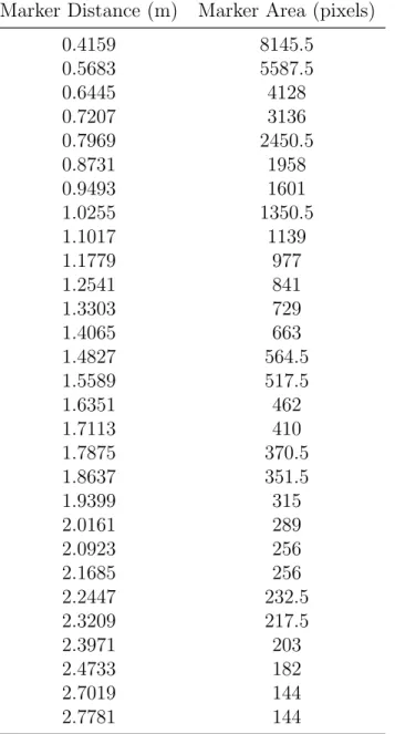
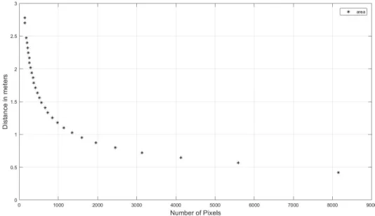
The objective of the experiment was to demonstrate that range can be calculated to a fair degree of accuracy based only on the relationship between the number of pixels of a feature with a known feature size, and the feature’s distance from the sensor. The marker area and distance from each image are tabulated in Table 9. When the marker distance is plotted as a function of pixel area, as in Figure 25, a correlation becomes apparent.

The MATLAB Curve Fitting Toolbox has many different models that can be used to describe variable relationships. When each curve model was tuned to fit the training data, the Exponential 2, Power, and Rational models all appeared to fit the data correctly. To quantitatively determine the optimal model, the RMSE was calculated. The equations for each fit model, as well as the RMSE when using that model, are listed in Table 10. This approach to calculate goodness of fit provided a definitive answer: the 1-2 rational fit model had the lowest RMSE error of 0.0200.

(68)

Table 9: Marker distance and area used to create a distance estimation

model for a 82mm×82mm marker.

Marker Distance (m) Marker Area (pixels) 0.4159 8145.5 0.5683 5587.5 0.6445 4128 0.7207 3136 0.7969 2450.5 0.8731 1958 0.9493 1601 1.0255 1350.5 1.1017 1139 1.1779 977 1.2541 841 1.3303 729 1.4065 663 1.4827 564.5 1.5589 517.5 1.6351 462 1.7113 410 1.7875 370.5 1.8637 351.5 1.9399 315 2.0161 289 2.0923 256 2.1685 256 2.2447 232.5 2.3209 217.5 2.3971 203 2.4733 182 2.7019 144 2.7781 144

(69)

Figure 25: Training data used to model the area-distance relationship for

an 82mm×82mm marker.

This was less than half of the error produced by using the Exponential model, and slightly better than the Power model. Figure 26 shows the tuned fit model overlaid on the training data set.

The accuracy of using a model with these tuning parameters was unknown. Addi-tional tests using images taken with known marker distances were required to deter-mine the accuracy of the method. More images of the marker were taken using two different distance intervals. The true distances with respect to pixel area from the new images were compared to the estimated distance calculated by using the model. As hypothesized, the new data follows the same relationship as the training data and the rational fit model. These three data sets are shown in Figure 27. The measure-ment error, shown in Figure 28, is the estimated distance from the model subtracted from the measured distance. All of the distances calculated when using this method were within 0.055 m of the measured value.

(70)

Table 10: Goodness of fit for different curve models based on RMSE of

the 82mm×82mm marker data.

Fit Model Fit Equation RMSE Polynomial 1 y=p1x+p2 0.4518 Polynomial 2 y=p1x2+p2x+p3 0.3235 Polynomial 3 y=p1x3+p2x2 +. . .+p4 0.2232 Weibull y=abxb−1_×_e−axb 1.7612 Exponential 1 y =aebx 0.2661 Exponential 2 y=aebx₊_cedx _0.0427

Fourier 1 y=a0+a1cos(xp) +b1sin(xp) 0.4481

Gaussian 1 y =a1e −(x−b1 c₁ ) 2 N/A Power 1 y=axb _0.0226 Power 2 y=axb₊_c _0.0230 rat12 y= _x2p1₊∗_q1x_∗+_xp2₊_q2 0.0200