Procedia Computer Science 46 ( 2015 ) 417 – 424
Available online at www.sciencedirect.com
1877-0509 © 2015 The Authors. Published by Elsevier B.V. This is an open access article under the CC BY-NC-ND license (http://creativecommons.org/licenses/by-nc-nd/4.0/).
Peer-review under responsibility of organizing committee of the International Conference on Information and Communication Technologies (ICICT 2014) doi: 10.1016/j.procs.2015.02.039
ScienceDirect
International Conference on Information and Communication Technologies (ICICT 2014)
Fuzzy clustering algorithms for cDNA microarray image spots
segmentation.
Biju V.G.
a,*, Mythili. P
baAssociate Professor, C.E. Munnar and Research Scholar, Division of Electronics, School of Engineering, CUSAT, Cochin-22, India b Associate Professor, Division of Electronics, School of Engineering, CUSAT, Cochin-22, India
Abstract
cDNA microarray image provides useful information about thousands of gene expressions simultaneously. Hence microarray image segmentation is an important task. In this paper, existing fuzzy clustering image segmentation methods in the literature have been tested for its suitability to perform segmentation of noisy cDNA microarray images. The algorithms considered for this purpose include fuzzy clustering based methods like, Fuzzy c-means (FCM), Possibilistic c means (PCM), Possibilistic fuzzy c means (PFCM) and Fuzzy local information c means (FLICM). The results of segmentation shows that FLICM is better in segmenting microarray spots compared to the other under the presence of noise.
© 2014 The Authors. Published by Elsevier B.V.
Peer-review under responsibility of organizing committee of the International Conference on Information and Communication Technologies (ICICT 2014).
Keywords: gene expression; clustering; spatial information; local information; image segmentation
1. Introduction
The initiation of microarray imaging technology has helped the scientist to effectively view the expression levels of thousands of gene at a time, which led to the expansion of studies in the life science.1,2,3 The spots on a microarray are segmented from the background to compute the gene expression. The three basic operations to compute the spot intensities are gridding, segmentation and intensity extraction.
* Corresponding author. Tel.: +919447234843.
E-mail address: [email protected]
These operations are used to find the accurate location of the spot, separate spot foreground (FG) from background © 2015 The Authors. Published by Elsevier B.V. This is an open access article under the CC BY-NC-ND license
(http://creativecommons.org/licenses/by-nc-nd/4.0/).
Peer-review under responsibility of organizing committee of the International Conference on Information and Communication Technologies (ICICT 2014)
(BG) and the calculation of the mean red and green intensity ratio for gene expression.
For microarray image analysis several software packages and algorithms were developed during the last decade. ScanAlyze Software uses a fixed circle segmentation algorithm for segmenting microarray spots, analysed each spot with a circle of fixed radius.4 An adaptive circle segmentation technique was employed in the GenePix software5, where the radius of each spot was not considered constant but adapts to each spot separately. Dapple software estimated the radius of the spot using the laplacian based edge detection.6 An adaptive shape segmentation technique was used in the Spot software.7 A histogram-based segmentation method was used in the ImaGene software 8, Later Watershed 9 and the Seeded region growing algorithms were employed10. The disadvantage of the above mentioned software packages and algorithms were either the spots were considered to be circular in shape or a priori knowledge of the precise position of the spot’s center was a prerequisite.11 Further segmentation algorithms based on the statistical Mann–Whitney test were also used12, which assess the statistical significant difference between the FG and BG. The K-means, Fuzzy c mean (FCM) and Genetic algorithm based fuzzy c mean algorithms (GAFCM) were the clustering algorithms used for microarray spot segmentation.13,14,15
The existing microarray spot segmentation algorithms show poor performance under noise. In order to avoid these limitations, in this paper, existing fuzzy clustering image segmentation algorithm have been tested for its suitability to segment cDNA microarray images in the presence of noise. The fuzzy clustering algorithms such as FCM14, Possibilistic c mean (PCM)16, Possibilistic fuzzy c means (PFCM)16, and Fuzzy local information c mean (FLICM)17 are used for microarray spot segmentation. Gridding of microarray image is done based on an original genetic algorithm approach for automatic gridding.18 For evaluation and testing of the algorithm both simulated and real microarray images are used. The performance of the algorithms are tested by evaluating the segmentation matching factor (SMF), Probability of error () and Normal mean square error (NMSE).
2. Fuzzy clustering
The aim of microarray image processing is to separate the FG and BG of each spot and then extract the intensity information from it. This is done through 3 steps 1. Gridding 2.Segmentation and 3.Intensity extraction. To address each spots in the image, gridding is done. Segmentation will separate the FG and BG of each spot. The intensity extraction will find the intensity of red and green information of the FG. The logarithmic value (base 2) of the ratio of intensities is the gene expression. These results are useful for accurate microarray analysis which involves data normalization, filtering and data mining. Fuzzy clustering is one of the most significant techniques that is used for segmentation and is applied in microarray images. The idea of clustering application is to divide the pixels of the image into several clusters (usually two clusters) and characterize these clusters as signal or background. The fuzzy clustering algorithms such as FCM, PCM, PFCM and FLICM are coded using matlab19 and used for spot segmentation of cDNA microarray images.
2.1 Possibilistic fuzzy c means (PFCM)
The PFCM 16 is a hybrid version of FCM and PCM. 14,16 It enjoys the benefits of both models. It solves the noise sensitivity defect of FCM and overcomes the coincident clustering problem of PCM. The FCM clustering algorithm was first introduced by Dunn and later extended by Bezdek. Let ݔ݅ ൌ ͳݐܰbe the pixels of a single
microarray spot, where N is the total number of pixels present in the spot image. These pixels have to be clustered in two classes BG and FG. Let݆ܿ ൌ ͳǡʹ be the prototype cluster centers of the FG and BG pixels respectively. A
membership function ݑrepresents the membership value of each pixel to be in different clusters. Based on the
maximum value of the membership function each pixel is grouped. The cluster centers are updated iteratively based on the grouped pixel. FCM is an iterative clustering algorithm that produces an optimal ܿ partitions by minimizing the weighted within group sum of squared error objective function ܨ௧
ࡲ࢚ൌ σ σ ࢛ ࢉ ୀ ࢊ א ሾǡሿ ࡺ ୀ (1)
ࢊൌ ቚห࢞െ ࢉหቚ
(2)
Hence the algorithm aims at iteratively improving the membership degree function until there is no change in the cluster centers. The sum of the membership values of a pixel belonging to all clusters should satisfy the following
equation.
σࢉୀ࢛ൌ ൌ ǡ ǡ ǥ Ǥ ࡺ (3)
The aim of this method is to minimize the absolute value of the difference between the two consecutive objective functions ܨ௧and ܨ௧ାଵ given by the equation 4.
ȁȁࡲ࢚ାെ ࡲ࢚ȁȁ ࢿ (4)
where ݉ is the fuzziness parameter and ߝ is error which has to be minimized. Iteratively in each step, the updated membership ݑ and the cluster centers ܿ are given by the following equations.
࢛ൌ σసሺࢊȀࢊሻȀሺషሻ (5) ࢉൌ σࡺస࢛࢞ σࡺస࢛ (6)
In FCM the membership of each pixel ݔ is inversely related to the relative distance between ݔandܿ. In microarray images ݆ ൌ ʹ, i.e. FGand BG, so when ȁȁݔെ ܿଵȁȁ=ȁȁݔെ ܿଶȁȁ these pixel xihas to be given equal membership in each clusters i.e. 0.5 irrespective of the low value or high value of these pixels and these creates noise points or outliers in FCM. To avoid this, Krishnapuram and Kellar proposed a new clustering model named PCM. 20
In PCM, which is an improved version of FCM, the constraint in equation 2 is relaxed to facilitate a possibilistic interpretation of the membership function. In other words, each pixels of the ݆௧ column can be any number between zero and one, so long as at least one of them is positive. The value of ݑ has to be interpreted as the typicality of ݔ relative to cluster ݆ (rather than its membership in the cluster). Each row of ݐwas interpreted as a possibility over
ݔ. The objective function in PCM is given by equation 7.
ࡲ࢚ൌ σ σ ࢚ ࢉ ୀ ࢊ σࢉୀࢽσࡺୀሺ െ ࢚ሻ א ሾǡሿ ࡺ ୀ (7) where ݐ is called the typicality of the pixel, each row of ݐ is interpreted as the possibility distribution over ݔ. ݐis calculated by equation 8.
ܜܑܒൌ
ାሺ܌ܑܒȀࢽሻȀሺܕషሻ (8)
where ߛ is a constant and is given by equation 9.
ࢽܑൌ ۹
σۼܑసܝܑܒܕࢊ
σۼܑసܝܑܒܕ ࡷ Ͳ (9) where ܭ is a constant greater than zero and ݑis obtained using equation 5. The cluster centers ܿis given by equation 10.
܋ܒൌ σۼܑసܜܑܒܕܠܑ
PFCM is a hybrid of FCM and PCM and enjoys the benefits of both models. PFCM solves the noise sensitivity defect of FCM and overcomes the coincident clustering problem of PCM. It is an iterative algorithm that tries to minimize the objective function given by equation 11. The cluster centers ܿ is given by equation 12.
ࡲ࢚ൌ σ σ ሺࢇ࢛ ࢉ ୀ ࢈࢚ ࣁ ሻࢊ σࢉ ࢽ ୀ σࡺୀሺ െ ࢚ሻࣁ ࡺ ୀ (11) ࢉൌσ ሺࢇ࢛ ା࢈࢚ ࣁ ሻ ࡺ స ࢞ σࡺసሺࢇ࢛ା࢈࢚ࣁሻ (12)
where ݑ is the membership function given by equation 5, ݐ is called the typicality of the pixel obtained by equation 8 and 9, ݉Ƭߛ are the fuzziness parameters, ܽƬܾ are constants with value equal to or greater than one. In PFCM16, the advantages and disadvantages of fuzzy clustering algorithms such as FCM and PCM methods were mathematically analyzed and a hybrid method PFCM was presented. The paper had compared various aspects of FCM, PCM and PFCM with four numerical data sets X10 ,X12 ,X400 ,X550 and one image dataset IRIS. For all data sets the maximum number of iterations was taken as 100. The number of clusters was taken as 3 for IRIS and 2 for all other data sets.
2.2 Fuzzy local information c means (FLICM)
FLICM is a modified version of FCM which makes use of fuzzy local similarity measure, aiming to guarantee noise insensitiveness and image details preservation. In order to enhance the insensitiveness to noise, a new factorܩ is included in FCM objective function.17 This factor incorporates local gray level and local spatial information in a fuzzy way so as to obtain robustness and noise insensitiveness, and also control the influence of the neighbourhood pixels depending on their distance from the central pixel.
ࡳൌ σ ࢊାሺ െ ࢛ሻ ฮ࢞ െ ࢉฮ ୀࡺ (13)
where the ݇௧pixel is the center of the local window, ݆ is the reference cluster and the ݅௧pixel belongs to the set of
neighbours falling into a window around the ݇௧ pixel ܰ
. ݀is the spatial Euclidean distance between pixels ݇Ƭ݆,
ݑis the degree of membership of the ݅௧ pixel in the ݆௧cluster, ݉ is the weighting exponent on each fuzzy
membership, and ܿis the prototype of the centre of cluster ݆. Local grey level and spatial information are included
in the objective function and is given by equation 14. ࡲ࢚ൌ σ σ ൣ࢛ ࢊ ࡳ൧ ࢉ ୀ ࡺ ୀ (14)
where the membership function and ݑcenter ܿ are obtained by equation 15 and 16. ܝܑܒ σ ൬܌ܑܒశ۵ܑܒ ܌ܑܓశ۵ܑܓ൰ Ȁሺܕషሻ ܋ ܓస (15) ܋ܒൌ σۼܑసሺܝܑܒܕሻܠܑ σۼܑసሺܝܑܒܕሻ (16)
The objective function Ft has to be minimized to find the optimum cluster centers. It can be obtained through an iterative process. The FLICM algorithm is given as follows.
Step 1. Initialize the cluster centers cj, fuzzification parameterሺሻand the stopping conditionሺɂሻ. Step 2. Find uij from equation 5 of FCM. Step 3. Set the loop count iter=0 Step 4. Compute fuzzy partition membership degree matrix uij using equation 15. Step 5. Calculate ୨ using equation 16. Step 6. Compute objective function ܨ௧ using equation 14.
Step 7. If the max ሼȁȁܨ௧ାଵെ ܨ௧ȁȁሽ ߝ then stop otherwise iter = iter+1 and go to step 4.
In FLICM17, the efficiency and the robustness of the method was compared with six fuzzy algorithms FCM S1, FCM S2, EnFCM, FGFCM S1, FGFCM S2, FGFCM, and two well-known non-fuzzy algorithms, k-means and SLINK algorithm. The performance of the algorithm was compared by presenting numerical results and examples on various synthetic and real images, with different types of noise. The synthetic test image used was a 128×128 pixel image with two gray level values taken as 20 and 120 and corrupted by different levels of Gaussian, Uniform and Salt & Pepper noise respectively. The number of clusters was taken as 2. The real image includes coin, wheel and flower images. The de noising performances of the above nine algorithms were compared with respect to the optimal segmentation accuracy (SA) and fuzzy similarity measure (ݎ). SA is defined as the sum of the correctly classified pixels divided by the sum of the total number of pixels. ݎ is a measure indicating the degree of equality between ܣ and ܥ, ܣrepresents the set of pixels belonging to the ݅௧ class found by the algorithm, while ܥ
represents the set of pixels belonging to the ݅௧class in the reference segmented image.
3. Database used 3.1 Synthetic database
A set of 40 microarray images, each with 225 spot, are simulated by the authors as mentioned in the literature 21,22 for numerically evaluating and comparing the various segmentation methods. In order to generate spots with realistic characteristics, the following procedure is adopted. Real cDNA sub array images are used as templates. Its binary version is produced by employing a suitable threshold. The address of each spot are identified by gridding. The intensities of each FG region is drawn from a uniform distribution whose mean value is taken as original spot mean value. The remaining BG pixel intensities are drawn from a uniform distribution whose mean intensity is determined from the original image. Note, all the BG intensities is drawn from a single distribution while FG intensities of each target region are drawn from an uniform distribution whose mean is estimated separately from the original respective spot region. The spots in microarray images sometimes exhibited doughnut-like shapes. During the simulation the doughnut holes which are identified as BG during thresholding, have the same intensity distributions as the BG.
3.2 Real microarray images
Real microarray images with category cell line & sub category drug treatment are downloaded from the UNC microarray data base.23 Each image consists of 34 blocks or sub arrays with each block containing 625 spots. From the downloaded images we have arbitrary selected 25 microarray blocks, i.e. total 15625 spots are used for segmentation. Although the ground truth is not known, it is clear from the segmentation result that the proposed method is more efficient in segmenting the real microarray spots.
4. Measures used for evaluation
To compare the performance of the fuzzy clustering algorithm applied on a synthetic database the following parameters are used. The synthetic database is evaluated with three parameter such as probability of error , segmentation matching factor (SMF), and Normal mean square error (NMSE). The synthetic database
images are corrupted by Additive white gaussian noise (AWGN)21,22 with the Signal-to-noise ratio (SNR) ranging from 1 to 10 dB. The segmentation ability of the FLICM algorithm is compared with FCM, PCM and PFCM by
finding the Segmentation matching factor (SMF), Probability of errorሺ), and Normal mean square error (NMSE) for every binary spots produced by these clustering algorithms.
The pixel-level accuracy of the segmentation is examined with the statistical parameter probability of error ǡ which measures the missegmented pixels, and is defined as2,24
ࢋൌ ࡼሺࡲሻࡼ ቀ
ࡲቁ ࡼሺሻࡼ ቀ ࡲ
ቁ (17) where ܲ ቀ
ிቁ is the probability of error in classifying foreground pixel as background pixels, ܲ ቀ ி
ቁis the probability of error in classifying background pixels as foreground pixels, ܲሺܨሻ and ܲሺܤሻ are a priori probabilities of foreground and background pixels in the image. The minimum value of zero occurs for when all of the pixels of the spots are segmented correctly. A maximum value of one for indicates a situation where all of the pixels of the background are segmented as foreground and vice versa. The Segmentation matching factor (SMF) 21,22 for every binary spot, produced by the clustering algorithm is given by
ࡿࡹࡲ ൌሺ࢙ࢋࢍתࢇࢉ࢚ሻ
ሺ࢙ࢋࢍࢇࢉ࢚ሻכ (18)
where Asegis the area of the spot, as determined by the proposed algorithm and Aact is the actual spot area. A perfect match in the case of SMF is indicated by a 100% score, any score higher than 50% indicates reasonable segmentation where as a score less than 50% indicate poor segmentation.21,22
For a simulated image with known ground truth, another metric called Normalized mean square error (NMSE)25 is used to measure the performance of the proposed approach which is given by
ࡺࡹࡿࡱ ൌට ࡹࡺσ σ ሺ࢞ࡹ ࡺ ି࢞തതതതሻଙଚ ࡹࡺσ σ ሺ࢞ࡹ ࡺ ሻ (19)
where M and N are the dimensions of the image. ݔ and ݔതതതതపఫ are the original and clustered image pixels respectively. NMSE is calculated for varying noise levels in the input image. A minimum value of zero is desirable for better segmentation.
5. Results and Discussion
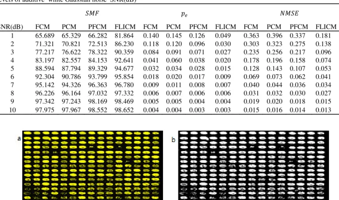
After validating the fuzzy clustering algorithms and ensuring its correctness, it is applied on a synthetic database. The synthetic microarray dataset includes a set of 40 images, each with 225 spots which is simulated as mentioned in the literature.21,22 Table 1 summarizes the average performance results obtained for segmenting spots of 40 simulated microarray images (10000 spots). The Fig. 1.a shows a simulated microarray image and Fig. 1. b shows the segmentation result obtained using the FLICM algorithm. The segmentation algorithm is applied on each image after applying the AWGN noise. The SNR value of noise is varied from 1 to 10 dB. The performance measurement parameter such as Segmentation matching factor (ܵܯܨ), Probability of errorሺሻ, and Normalized mean square error (ܰܯܵܧ) achieved for all simulated spots corresponding to different SNR levels are presented in Table 1.Regarding the ܵܯܨ, the FLICM algorithm resulted in higher spot area identification accuracy than FCM, PCM and PFCM.
The ultimate goal of the segmentation process in microarray image processing is to obtain intensity measurement. Accurate segmentation of spot has a great impact on the intensity calculation. Measurements based on the pixel intensity, rather than the segmentation area such as Probability of error ( ) and Normalized mean square error (ܰܯܵܧ), support the superiority of the FLICM against FCM, PCM and PFCM. When evaluating the results in intensity extraction perspective a lower value of and NMSE are expected for the better performance of the algorithm. 12 Hence the FLICM is better compared to other algorithms
Real microarray images downloaded from the UNC microarray data base24 is used for segmenting spots FG from BG. All downloaded images are having 34 sub arrays with 625 spots in each sub array. The FLICM algorithm is applied on 25 such sub arrays. The Fig. 2. a shows a real image sub array obtained from the UNC microarray data base and Fig. 2 .b shows segmentation result using FLICM algorithm for real cDNA microarray image.
Fig. 1(a) A microarray simulated image with 225 spots; (b) Segmentation result obtained for the FLICM algorithm
Fig. 2(a). Real cDNA microarray image; (b) Segmentation result using FLICM algorithm for real cDNA microarray image.
6. Conclusion
Table 1. The comparison of FCM, PCM, PFCM, FLICM algorithm based on segmentation matching factor (ܵܯܨ), Probability of error () and Normalized mean square error (ܰܯܵܧ) for simulated microarray images with different
levels of additive white Gaussian noise SNR(dB)
ܵܯܨ ܰܯܵܧ
SNR(dB) FCM PCM PFCM FLICM FCM PCM PFCM FLICM FCM PCM PFCM FLICM 1 65.689 65.329 66.282 81.864 0.140 0.145 0.126 0.049 0.363 0.396 0.337 0.181 2 71.321 70.821 72.513 86.230 0.118 0.120 0.096 0.030 0.303 0.323 0.275 0.138 3 77.217 76.622 78.322 90.359 0.084 0.091 0.071 0.027 0.235 0.256 0.217 0.096 4 83.197 82.557 84.153 92.641 0.041 0.060 0.038 0.020 0.178 0.196 0.158 0.074 5 88.594 87.794 89.329 94.677 0.032 0.034 0.028 0.015 0.128 0.143 0.107 0.053 6 92.304 90.786 93.799 95.854 0.018 0.020 0.017 0.009 0.069 0.073 0.062 0.041 7 95.142 94.326 96.363 96.780 0.009 0.011 0.008 0.007 0.040 0.044 0.036 0.034 8 96.226 96.164 97.032 97.332 0.006 0.007 0.006 0.006 0.031 0.032 0.030 0.027 9 97.342 97.243 98.169 98.469 0.005 0.005 0.004 0.004 0.019 0.020 0.018 0.015 10 97.975 97.967 98.552 98.652 0.004 0.004 0.003 0.003 0.015 0.016 0.014 0.013
In this paper, existing fuzzy clustering image segmentation methods available in the literature have been tested for its suitability to perform for better microarray spot segmentation under noise. The algorithms are tested on both simulated and actual cDNA microarray images. The number of spots in the synthetic images used for the evaluation purpose and measures obtained support the superiority of the FLICM method over other existing fuzzy clustering methods for microarray image processing.
References
1. Yang YH, Buckley MJ, Duboit S, Speed TP. Comparison of methods for image analysis on c DNA microarray data. J.Comput. Graphical Statist, 2002; 11: p.108–136.
2. Lehmussola A, Ruusuvuori P, YliHarja A. Evaluating the performance of microarray segmentation algorithms. Bioinformatics, 2006; 22: p.29102917. 3. Schena M, Shalon D, Davis RW, Brown PO. Quantitative monitoring of gene expression patterns with a complementary DNA microarray. Science, 270, 1995; p.467- 470.
4. Eisen M B, ScanAlyze, 1999, http://rana.lbl.gov/ EisenSoftware.htm.
5. GenPix 4000, A User’s Guide, Axon Instruments, Inc, Foster City,CA.6.Buhler J, Ideker T, Haynor, D. Dapple: improved techniques for finding spots on DNA microarrays, Technical Report. UWTR 2000; 08, 05, UV CSE, Seattle, Washington, USA.
6. Buhler J, Ideker T, Haynor, D. Dapple: improved techniques for finding spots on DNA microarrays, Technical Report. UWTR 2000; 08, 05, UV CSE, Seattle, Washington, USA
7. Buckley M.J. The spot user’s guide CSIRO Mathematical and Information Science,2000, http://www.cmis.csiro.au/IAP/Spot/spotmanual.html. 8. ImaGene, ImaGene 6.1 User Manual, http://www.biodiscovery.com/index/pappsweb files action. 9. Beucher S, Meyer F,Themorphological approach to segmentation The watershed transformation, Opt. Eng, 1993; 34, p. 433–481.
10. Adams R, Bischof L, Seeded region growing, IEEE Trans. Pattern Anal. Mach. Intel., 1994; 16, (6), p. 641–647.
11. Bozinov D, Rahenfuhrer J,Unsupervised technique for robust target separation and analysis of DNA microarray spots through adaptive pixel clustering, J. Bioinform, 2002; 18, p. 747-756.
12. Chen Y, Dougherty ER, Bittne ML. Ratio based decisions about the quantitative analysis of c DNA microarray images, J. Biomed.Opt, 1997;
2, p.264–374.
13. Wu S, Yan H. Microarray Image Processing Based on Clustering and Morphological Analysis in Proc. Of First Asia Pasific Bioinformatics Conference, Adelaide, Australia, 2003; p. 111-118.
14. Volkan U, Ĉhsan, OB. Microarray image segmentation using clustering methods, Mathematical and Computational Applications 15, (2) p.2 40-247.
15. Biju VG, Mythili P. A Genetic Algorithm based Fuzzy C Mean Clustering Model for Segmenting Microarray Images, International Journal of Computer Applications, 2012; 52, (11), p.42-48.
16. Nikil RP, Kuhu P, James MK, James CB. A Possibilistic Fuzzy CMeans Clustering algorithm, IEEE Trans on Fuzzy systems, 2005;13,(4), p. 517-530.
17. Krinidis S, Vassilios C.A Robust Fuzzy Local information C Means Clustering algorithm, IEEE Transaction Image Processing 2010;19,5. 18. Zacharia E, Maroulis D. An original Genetic approach tofully automatic gridding of microarray images, IEEE transaction on medical imaging, 2008; 2796, p.805-813.
19. The Math Works, Inc., Software, MATLABR (2010a), Natick, MA.
20. Krishnapuram R, Kellar JA. Possibilistic approach to clustering, IEEE Trans, Fuzzy Systems, 1993; 4,(3), p.98-110.
21. Athanasiadis EI, Cavouras DA, Spyridonos PP, Glotsos DT, Kalatzis IK, Nikiforidis GC. DNA microarray image processing based on the Fuzzy Gaussian mixture model, IEEE Transaction on Information Technology in Biomedicine,2009;13,issue 4.
22. Athanasiadis EI, Cavouras DA, Spyridonos PP, Glotsos DT, Kalatzis IK, Nikiforidis GC. A Wavelet based markov random field segmentation mode in segmenting microarray experiments, Computer methods and programs in biomedicine, 2011;104, p. 307- 315. 23. UNC Microarray database. https://genome.unc.edu
24. Zacharia, E., Maroulis,D. 3 D Spot Modeling for Automatic Segmentation of cDNA Microarray Images, IEEE,Transactions on Nano Bioscience ,2010, 9, (3), p 181-192
Ϯϱ͘Ping WYU, Maheshwar G. A comparison of fuzzy clustering approaches for quantification of Microarray Gene expression Journal for signal processing systems, 2008;50,( 3), p. 305-320.