P
ORTFOLIO SELECTION USING
ARTIFICIAL INTELLIGENCE
Andrew J Ashwood
BEng(Civil)(Hons), LLB, GradCertLaw, LLM, MBA
Submitted in partial fulfilment of the requirements for the degree of Doctor of Business Administration (BS25)
QUT Business School
Queensland University of Technology June 2013
Portfolio selection using artificial intelligence i
Keywords
Neural network, artificial neural network, portfolio selection, performance measurement, efficient market hypothesis, Four-factor model, alpha, feed-forward, back-propagation
ii Portfolio selection using artificial intelligence
Abstract
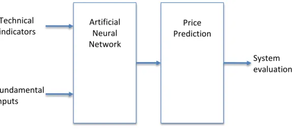
Artificial neural networks (‘ANNs’) were created and then used to predict future price returns of 20 widely held ASX200 stocks along with equally weighted and value weighted portfolios of these stocks. Network testing was undertaken to investigate several network parameters including (1) input type, (2) hidden layer size, (3) lookback window, and (4) training period length. This testing did not provide useful guidance on heuristics for the input type, lookback window, or training period length. The hidden layer size, while still demonstrating a degree of variability between stocks, generally performed better at the low end of the testing range. Almost half of the optimal network models utilised the smallest hidden layer of 30 nodes.
The ANN price predictive capability was tested ever a 10 year period from the beginning of 2002 to the end of 2011. Network performance was mixed. For some stocks the networks performed relatively well, predicting future prices with error at or below 5% for several years in a row. However even these relatively well performing models generally performed poorly at the beginning and end of the global financial crisis (beginning of 2008 and end of 2009 respectively).
Stock directional movement prediction performance was assessed. Over the 10 year testing horizon the ANN models predicted directional movement with better than 50% accuracy for all stocks and portfolios except for BHP. Significant results were achieved for 13 of the 22 stocks and portfolios tested.
The most accurate network specification for each stock was then used to form long and long-short portfolios. Performance measurement using the Carhart four-factor model indicated that both portfolios achieved positive alpha. These positive
Portfolio selection using artificial intelligence iii results however relied on post hoc information. To address this concern, a distribution of alpha for all 600 different network specifications was produced. Analysis indicated that the distribution of alpha was normally distributed. The distribution of alphas demonstrated that about 88% of the network models produced abnormal risk adjusted returns. The alpha value was significant in 27% of cases where the network achieved positive alpha. None of the negative alpha values were statistically significant.
The Carhart four-factor model was used to assess the simulated returns of the ANNs to determine if the known style factors significantly predicted the simulated prices produced by the ANNs. The analysis showed for 7 of the 22 stocks and portfolios, the Carhart four-factor model significantly predicted simulated price returns.
iv Portfolio selection using artificial intelligence
Table of Contents
Keywords ... i Abstract ... ii Table of Contents ... iv List of Figures ... viList of Tables ... vii
List of Abbreviations ... ix
Statement of Original Authorship ... x
Acknowledgements ... xi Chapter 1: Introduction... 1 Background ... 4 Motivation ... 4 Research contribution ... 5 Australian data ... 5
Broad testing horizon ... 6
Performance measurement ... 6
Network parameter testing ... 7
Range of network inputs tested ... 7
Chapter 2: Neural Network Primer ... 9
The biological network ... 9
The artificial neuron ... 11
The artificial neural network ... 13
Neuron activation ... 14 Neuron Transformation ... 15 Transformation functions ... 15 Threshold function ... 16 Ramp function ... 16 Linear function... 17 Sigmoid function ... 17
The Complete Model of an Artificial Neuron ... 18
Neural Networks ... 18
Network learning ... 20
Error Functions ... 21
Back Propagation ... 22
Network architecture... 28
Chapter 3: Literature review ... 30
Why use artificial neural networks ... 30
Neural networks in finance research ... 32
Efficient market hypothesis ... 50
Chapter 4: Research ... 54
Research questions ... 54
Portfolio selection using artificial intelligence v
Secondary Research Question 1 ... 55
Secondary Research Question 2 ... 55
Secondary Research Question 3 ... 55
Research design/methodology ...55
The Kaastra 8 step process ... 55
Variable selection/Network Inputs ... 56
Data set ... 60
Data pre-processing... 79
Frequency of data ... 81
Training, testing and validation sets ... 82
Neural network paradigm/structure ... 88
Evaluation criteria ... 94
NN training ... 94
Implementation ... 97
Chapter 5: Analysis ... 103
Network Configuration Analysis ...103
Input type ... 103
Hidden layer size... 104
Lookback window length ... 106
Training period length ... 106
MSE of each model ...107
Correct directional movement prediction ...113
Trading system and performance measurement ...116
Portfolio construction ... 116
Performance measurement ... 117
Chapter 6: Conclusions ... 127
Link to Finance Theory ...130
Limitations of the study ...133
Bibliography ... 136
Appendices ... 142
vi Portfolio selection using artificial intelligence
List of Figures
Figure 1 Typical biological neuron (Fraser, 1998) ... 9
Figure 2 Block diagram representation of human nervous system ... 10
Figure 3 McCulloch-Pitts Perceptron model ... 11
Figure 4 Rosenblatt Perceptron ... 13
Figure 5 Typical neural processing element ... 14
Figure 6 Neuron summing calculation ... 15
Figure 7 Complete model of an artificial neuron ... 18
Figure 8 Typical 3-layer fully connected feed-forward ANN ... 20
Figure 9 Multi-layer feed-forward network ... 24
Figure 10 Schematic of proposed study ... 54
Figure 11 Kaastra & Boyd (1996) 8 step design framework ... 56
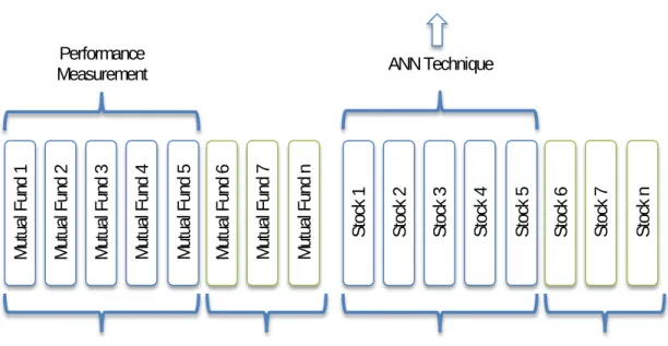
Figure 12 Diagrammatic representation of this study compared with typical performance studies ... 63
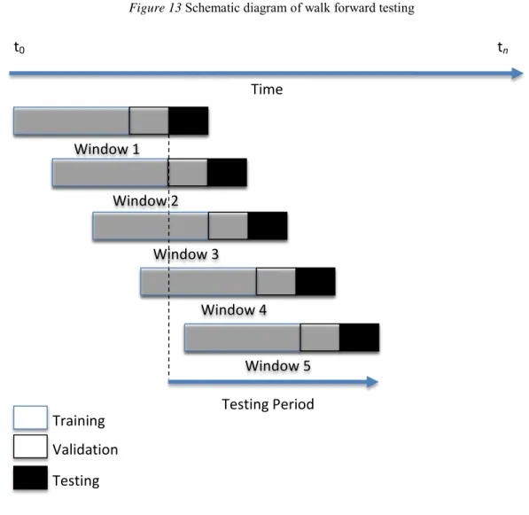
Figure 13 Schematic diagram of walk forward testing ... 84
Figure 14 Schematic diagram of artificial neural network implementation ... 101
Figure 15 Histogram of optimum input type ... 104
Figure 16 Histogram of optimum hidden layer size ... 105
Figure 17 Histogram of optimum look back window ... 106
Figure 18 Histogram of optimum training period length ... 107
Figure 19 ASX200 from 2002 to 2011 ... 111
Figure 20 Histogram of alpha ... 125
Portfolio selection using artificial intelligence vii
List of Tables
Table 1 Jang & Lai (1994) results ... 45
Table 2 Comparison of EMH categories as defined by Fama 1970 and 1991 ... 52
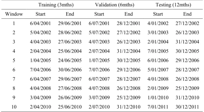
Table 3 Walk forward testing (3mth training period) ... 86
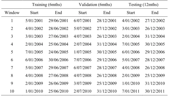
Table 4 Walk forward testing (6mth training period) ... 87
Table 5 Walk forward testing (12mth training period) ... 87
Table 6 Walk forward testing (24mth training period) ... 88
Table 7 Heuristics to estimate hidden layer size ... 91
Table 8 Dynamic network testing parameters ... 98
Table 9 Static network testing parameters ... 99
Table 10 Network performance results ... 109
Table 11 Network performance results (cont'd) ... 110
Table 12 Directional movement prediction performance ... 114
Table 13 Directional movement prediction performance (cont'd) ... 115
Table 14 Regression analysis for the most accurate ANN ... 121
Table 15 Regression analysis for the median ANN ... 122
Table 16 Descriptive statistics for alpha ... 124
Table 17 AMC Regression Analysis ... 142
Table 18 ANZ Regression Analysis ... 143
Table 19 BHP Regression Analysis ... 143
Table 20 CBA Regression Analysis ... 144
Table 21 CCL Regression Analysis ... 145
Table 22 CSL Regression Analysis ... 145
Table 23 DJS Regression Analysis ... 146
Table 24 GPT Regression Analysis ... 147
Table 25 LEI Regression Analysis ... 147
Table 26 NAB Regression Analysis ... 148
Table 27 ORG Regression Analysis ... 149
Table 28 QAN Regression Analysis ... 149
Table 29 QBE Regression Analysis ... 150
Table 30 RIO Regression Analysis ... 151
Table 31 SUN Regression Analysis ... 151
viii Portfolio selection using artificial intelligence
Table 33 WBC Regression Analysis ... 153
Table 34 WDC Regression Analysis ... 153
Table 35 WES Regression Analysis ... 154
Table 36 WOW Regression Analysis ... 155
Table 37 EW Regression Analysis ... 155
Portfolio selection using artificial intelligence ix
List of Abbreviations
ANN Artificial neural network
ASX Australian Securities Exchange
CAPM Capital Asset Pricing Model
EMA Exponential moving average
EMH Efficient market hypothesis
MA Moving average
MSE Mean squared error
RMSE Root mean squared error
ROC Rate of change
S&P Standard & Poors
x Portfolio selection using artificial intelligence
Statement of Original Authorship
The work contained in this thesis has not been previously submitted to meet requirements for an award at this or any other higher education institution. To the best of my knowledge and belief, the thesis contains no material previously published or written by another person except where due reference is made.
Signature:
Date: 1/01/2014
Portfolio selection using artificial intelligence xi
Acknowledgements
My primary acknowledgement goes to Dr Anup Basu, my supervisor and mentor, without whom I would never have accomplished this research. I am greatly indebted to Anup.
I would like to formally thank and acknowledge the QUT High Performance Computing department.
I would like to thank Dr Robert Bianchi of Griffith University for supplying the Carhart regression factors. This saved me a significant volume of effort.
My final acknowledgement goes to my wife Eve, for being encouraging and supportive throughout the entire process.
Chapter 1: Introduction 1
Chapter 1:
Introduction
Trading in equities is big business in Australia. The market capitalisation of the 500 largest publicly listed corporations in Australia is approximately $1.2 trillion dollars.1 In the twelve month period to January 2013, 244 billion stocks of these top
500 Australian companies were traded. This is equivalent to 488 million stocks changing hands per stock per year or 1.3 million trades per stock per day on average over the year. The true averages are higher because the Australian Securities Exchange (“ASX”) does not trade on weekends and holidays. The turnover in the top 500 stocks in 2012 was over a trillion dollars.
By any measure, the value of Australia’s stock market is significant and the volume of trading activity demonstrates eagerness on the part of investors to buy and sell stocks in the hope of achieving above average returns. The figures above include only vanilla stock trades; the volumes and turnover are much greater if derivatives of these equities such as futures, options, and swaps are included. Malkiel (2011) states that “Professional investment analysts and counsellors are involved in what has been called the biggest game in town” (p.111).
Most Australians have a significant portion of their personal wealth invested in equities in the form of superannuation. The total amount currently invested in Australian superannuation funds has been estimated at $1.4 trillion (APRA, 2013). A large proportion of these funds are invested with active fund managers, managers who try to beat the market by actively choosing which stocks to buy and sell. But outperforming the broader market is difficult. There is limited research to support
1 As at 11/9/2012. For further information refer to - http://www.standardandpoors.com/indices/sp-asx-all-ordinaries/.
2 Chapter 1: Introduction skill on the part of these active managers (Fama & French, 2009; Karaban & Maguire, 2012; Steinfort & McIntosh, 2012). In Australia, 7 out of 10 actively managed retail funds underperformed the market index over both a one and three year horizon (Karaban & Maguire, 2012).
Forty years ago in 1973, Burton Malkiel authored ‘A Random Walk Down Wall Street’, a seminal work on market efficiency and the ability of financial experts to outperform the market. Malkiel (2011) makes the case for market efficiency in very simple terms:
An investor with $10,000 at the start of 1969 who invested in a Standard & Poor’s 500-Stock Index Fund would have had a portfolio worth $463,000 by 2010, assuming that all dividends were reinvested. A second investor who instead purchased shares in the average actively managed fund would have seen his investment grow to $258,000. The difference is dramatic. Through May 30, 2010, the index investor was ahead by $205,000, an amount almost 80 per cent greater than the final stake of the average investor in a managed fund. (p.17)
Malkiel eloquently makes the point that most actively managed funds fail to outperform the broader market. Fama and French (2009) in their paper ‘Luck versus Skill in the Cross Section of Mutual Fund Returns’ examine mutual fund performance from the equilibrium accounting perspective. They compared the actual cross-section of fund alpha (α) estimates to the results from 10,000 bootstrap simulations from the cross-section. They found very little evidence of skill on the part of active fund managers. Their results for the period from 1984 to 2006 show that mutual fund investors in aggregate, achieve returns that underperform the CAPM, three-factor, and four-factor benchmarks. Fama and French (2009) conclude:
Chapter 1: Introduction 3
For fund investors the simulation results are disheartening. When α is estimated on net returns to investors, the cross-section of precision-adjusted α estimates…suggests that few active funds produce benchmark adjusted expected returns that cover their costs. Thus, if many managers have sufficient skill to cover costs, they are hidden by the mass of managers with insufficient skill. On a practical level, our results on long-term performance say that true α in net returns to investors is negative for most if not all active funds... (p.2)
While Malkiel and Fama & French have examined the ability of active fund managers to outperform the US market, the evidence suggests that the Australian experience is no different. In the mid-2012 S&P Indices Versus Active Funds Scorecard Karaban and Maguire (2012) point out that over a one and three year investment horizon, 7 out of 10 actively managed Australian retail funds underperformed their relative benchmark. Over a five year investment horizon the retail funds performed slightly better but 2 out of 3 funds still underperformed the benchmark.
Notwithstanding the limited evidence of skill in outperforming the market, the astonishing technical advances in computing power over the past twenty years in combination with the widespread availability of historical data on the internet has provided with investors with increased opportunity to test markets for predictable returns. From a theoretical perspective, Artificial Neural Networks (‘ANNs’) have several traits that suggest their suitability for stock price prediction. ANNs have the ability to generalise and to learn. They provide an analytic alternative to other techniques that rely on strict assumptions of normality, linearity, and variable independence. The use of ANN in financial research has increased dramatically over
4 Chapter 1: Introduction the past two decades. For example, in a literature review of the field, Wong and Yakup (1998) examined the ABI/Inform database, the Business Periodical Index, 21 textbooks, and 12 journals for the period from 1971 to 1996 looking for evidence of research articles using the descriptors ‘neural network’ and its plural. They could not find any application of ANNs in finance published prior to 1990. However, by 1993 over ten articles per year were being published (Wong & Yakup, 1998).
Background
Financial research utilising artificial neural networks is a relatively new area with published research in the field only going back a little over twenty years. Over the period since neural networks have been used in financial research, the vast majority of the work has been applied to US stocks and indexes. Limited research has been undertaken in the Australian domain. For example Ellis & Wilson (2005) used ANNs in an Australian REIT context to identify value stocks. Tan (1997) used ANNs for financial distress prediction and as part of a foreign exchange hybrid trading system. Vanstone, Finnie and Hahn (2010) used fundamental inputs to create a filter rule based ANN for stock selection in an Australian context. Tilakaratne, Mammadov and Morris (2008) used ANNs to develop algorithms for predicting trading signals for the Australian All Ordinaries Index.
Motivation
Testing of stocks for predictability of return has been widely investigated. According to Malkiel:
The attempt to predict accurately the future course of stock prices and thus the appropriate time to buy or sell a stock must rank as one of investors’ most persistent endeavours. (p.112)
Chapter 1: Introduction 5 Ignoring transaction costs, this research intends to determine if neural networks can be successfully implemented to predict price and directional movement of widely held Australian stocks. Further, the study seeks to examine if these price predictions can be used for portfolio selection and whether these portfolios achieve positive alpha when measured using the Carhart 4-factor model.
Research contribution
A relatively new and computationally intensive approach to stock price prediction has been utilised in an effort to predict the future price of Australian equities. While there has been previous research using ANNs to try and predict future stock prices, the following discussion lists the components that in combination make this piece of research a significant contribution to the field.
Australian data
Very little research in the field involves the use of Australian data. As is typically found in the finance field, the vast majority of published work in the field focuses on the US market. While there has been some Australian research that has utilised ANNs, the current literature contains significant research gaps. For example, the existing Australian research focuses either on using ANNs for pattern recognition such as identifying value stocks (Ellis & Wilson, 2005) or creating a predictive filter rule (Vanstone et al., 2010) or for prediction of trading signals of the All Ordinaries
(Tilakaratne et al., 2008). None of the existing research in the Australian domain
utilises ANNs for price prediction of individual stocks. This research provides a significant contribution in that it is the first study to create an ANN price prediction model that utilises a combination of technical and fundamental input data to predict future prices of widely held Australian stocks and use these predicted prices for portfolio selection.
6 Chapter 1: Introduction Broad testing horizon
The bulk of the past literature has used short testing periods for neural networks. Freitas, Souza, Gomez and Almeida (2001) used a variant of the Markowitz mean-variance model with expected returns generated with ANNs to create portfolios using Brazilian stocks. While Freitas et al. (2001) achieved high
returns, the brief 21 week testing period utilised is not considered robust. Jang and Lai (1994) used ANNs for prediction of the Taiwan Stock Exchange over a two year testing period. Ko and Lin (2008) adopted a five year dataset, which included the training, validation, and only two years of testing data. Among the handful of studies that used longer testing horizons are Vanstone et al. (2010) who utilised a five year
testing horizon, while Tilakaratne et al. (2008) utilised a nine year testing horizon.
This study uses a fifteen year dataset with a ten year testing horizon. This is a significant contribution to the extant literature in terms of enhanced robustness in testing the network’s predictive ability.
Performance measurement
The majority of the previous research reports ANN returns on a raw basis only. The only studies that utilised some form of risk-adjustment were the Australian studies by Ellis and Wilson (2005) who report portfolio returns along with the Sharpe and Sortino ratios for the ANN portfolios and Vanstone et al. (2010) who reported
the Sharpe ratio for the ANN portfolio. None of the studies obtained during the literature review utilised a performance measurement framework to analyse if the results being achieved are due to any of the known style factors. For example, it is possible that a highly accurate predictive ANN model could achieve returns that exceed a benchmark index but do so by investing in riskier stocks. The ANN system in this case may not have achieved abnormal risk-adjusted returns; the ANN system may have merely identified the riskier stocks in which to invest. The existing body of
Chapter 1: Introduction 7 literature contains multiple examples of studies that report outperformance of the market without any reference to an established performance measurement framework (Freitas et al., 2001; Hall, 1994). To the author’s knowledge, this research is the first
in the field to utilise the Carhart four-factor model (Carhart, 1997) for both performance measurement.
Network parameter testing
Very little published research in the field provides information regarding how network configuration affects network predictive capability. Typically, the literature provides some details about the network configuration adopted, but provides little or no justification or information about how the configuration performs when benchmarked against other configurations. An example is the paper by Hall (1994) that reports that the performance of the ANN portfolio has exceeded the S&P500 net of transaction costs but then go on to state that actual performance results and specific details of the system are proprietary. While reliable heuristics exist for specification of some network parameters, others are unreliable and correct network specification relies on experimentation.
This study makes a significant contribution by providing high level examination and reporting on different network configurations with variable inputs, hidden layer size, lookback window, training period length.
Range of network inputs tested
Much of the previous research in the field typically uses only one type of network input in order to make predictions. For example, Ellis and Wilson (2005) took a pattern classification approach whereby accounting ratios were used to classify stocks as value or growth stocks. Tilakaratne et al. (2008) used close price
8 Chapter 1: Introduction Swales (1991) used a mixture of fundamental measures and macroeconomic indicators to classify stocks. Vanstone et al. (2010) used an ANN based on a filter
rule that used fundamental measures for portfolio selection. Jang and Lai (1994) utilised 16 different technical indicators (excluding past prices) in order to try and predict future stock prices. Kryzanowski, Galler and Wright (1992) used fundamental inputs only to try and predict stock price directional movement over the subsequent year.
While previous studies have utilised either past price or fundamental inputs or non-price based technical indicators as network inputs, this research utilises a combination of technical indicators and fundamental measures as networks inputs (59 inputs in total). In addition to using this broad cross section of inputs, network simulations are undertaken using different combinations of these inputs types to provide a high level insight into how each of the input types affects network predictive capability.
Chapter 2: Neural Network Primer 9
Chapter 2:
Neural Network Primer
The biological network
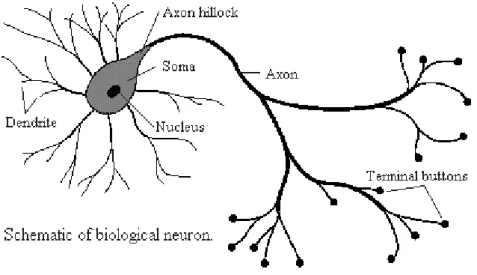
Biological brains are comprised of large numbers of cells called neurons. The neurons function as groups of several thousand which are called networks. Figure 1
Typical biological neuron (Fraser, 1998) shows the typical structure of a biological neuron.
Figure 1 Typical biological neuron (Fraser, 1998)
A biological neuron comprises a cell body (the soma) which contains the cell nucleus, a long thin structure called the axon, and hair like structures called dendrites which surround the soma. The soma is the central part of the neuron that contains the cell nucleus and is where the majority of protein synthesis occurs. The axon is a long cable-like structure which carries nerve signals from the soma. In biological networks, the axon of each cell terminates in small structures called terminal buttons which almost connect to the dendrites of other cells. The small gap in between these terminal buttons and dendrites of other neurons is called the synapse. Information is passed from one cell to another via the synapse.
10 Chapter 2: Neural Network Primer The neuron receives stimulus (input) from its network of dendrites. The input stimulus is then processed in the nucleus of the cell body. The neuron then sends out electrical impulses through the long thin axon. At the end of each strand of the axon is the synapse. The synapse is able to increase or decrease its strength of connection and causes excitation or inhibition in the connected neuron (Medsker & Liebowitz, 1994). In the biological brain, learning occurs through the changing of the effectiveness of the synapses so that the influence that one neuron has on its connected neurons changes (Stergiou & Siganos, 2010).
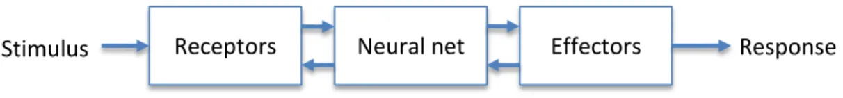
The human nervous system can be represented as a three stage model as shown in Figure 2 (Haykin, 1999). The central unit of the human nervous system is the
brain, which is represented by the neural net. The brain continually receives input information from receptors, processes the information, and makes decisions. The receptors convert the stimulus from the environment into electrical impulses that convey information to the brain. Once the brain has processed this input stimulus it provides a message to the effectors that convert these electrical impulses generated by the brain into system responses. The arrows pointing from left to right indicate a forward transmission of information signals through the system. The arrows pointing from right to left show the presence of feedback in the system.
Figure 2 Block diagram representation of human nervous system
Chapter 2: Neural Network Primer 11 The artificial neuron
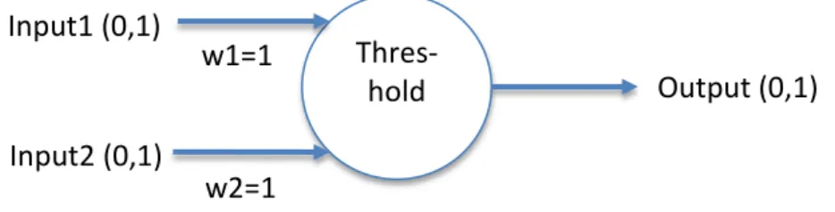
The first artificial neuron model was proposed by McCulloch and Pitts in 1943 (McCulloch & Pitts, 1943). Their paper suggested that neurons with binary inputs and binary threshold activation functions were similar to first order logic sentences.
Figure 3 McCulloch-Pitts Perceptron model
The McCulloch-Pitts neuron model used binary inputs (inputs of 0 which represented false/off and 1 which represented true/on) to create a binary threshold and neuron output. The neuron shown in Figure 3 has two inputs (Input1, Input2)
which are binary inputs (value is either 0 or 1). Each input contains an input weighting factor (w1 and w2) equal to one. The neuron contains a threshold function that is determined arbitrarily depending on the desired function and output of the neuron. The neuron also contains a single output which is also binary. This neuron model can be used to create truth tables and model simple functions such as AND, OR, NOT. The McCulloch-Pitts model was a highly simplified model that contained several constraints:
1. It could only accept binary inputs and provide binary outputs, 2. It had a fixed threshold,
3. It could only utilize identical input weights,
4. Inhibitory inputs had power of veto over excitatory inputs, and
5. At each time step the neuron is updated by simultaneously updating the excitatory inputs and setting the output to 1 if the sum meets the threshold level and there is no inhibitory input.
w2=1 w1=1 Thres-hold Input1 (0,1) Input2 (0,1) Output (0,1)
12 Chapter 2: Neural Network Primer The McCulloch-Pitts model was not tremendously useful at the time. While it could be used to implement any Boolean logic function, it had rigid limitations and did not have any learning ability. Therefore it offered little advantage over the existing digital logic circuits. The next major advance in the artificial neuron was proposed by Donald Hebb in 1949. Hebb (2002) postulated Hebb’s Rule,
Let us assume that the persistence or repetition of a reverberatory activity (or “trace”) tends to induce lasting cellular changes that add to its stability…When an axon of cell A is near enough to excite a cell B and repeatedly or persistently takes part in firing it, some growth process or metabolic change takes place in one or both cells such that A’s efficiency, as one of the cells firing B, is increased. (p.62)
Hebb’s theory attempted to explain the phenomenon of associative learning whereby the firing of one neuron generally leads to the firing of another neuron. Hebb’s Rule can be applied to the artificial neuron. Unlike the McCulloch-Pitts model where input weights are all identical, Hebb’s Rule provides a theoretical basis for altering weights between neurons. The weight factor can be increased where two neurons generally activate simultaneously and reduced in other situations.
Hebbian theory provided part of the basis for the next major advance which was the perceptron model proposed by Rosenblatt (1958). The perceptron proposed by Rosenblatt had several key differences from the McCulloch-Pitts model. Firstly, input weights were not all fixed at one. They could differ in value, range between different values, and also be negative. Secondly, inhibitory inputs no longer had an absolute power of veto over excitatory inputs. Thirdly, the perceptron contained a learning function based on Hebb’s Rule.
Chapter 2: Neural Network Primer 13 Figure 4 Rosenblatt Perceptron
Figure 4 shows the Rosenblatt perceptron. As can be seen, while the output is still two-state, the perceptron model allows for much greater flexibility in inputs (they are no longer binary) and weights (as each input now has a unique weight factor). The learning rule that was proposed to complete the perceptron model was the perceptron convergence algorithm. While a complete analysis of this algorithm is unnecessary, the input weights could be updated by following the procedure:
1. Check whether a calculated output has been correctly classified. If it has been correctly classified do nothing.
2. Otherwise update the input weight by a factor of the input, the input weight, and a learning-rate parameter.
The artificial neural network
Since these first models of the artificial processing element were postulated, developments in mathematics, statistics, and computer processing power allowed this model to be modified and widely applied in subsequent work (Mehrotra, Mohan & Ranka, 1997). Figure 5 Typical neural processing element shows the typical
structure of an artificial neural processing unit as found in most neural networks today. w2 w1 Thres-hold Input1 Input2 Output (0,1) or (-1, 1)
14 Chapter 2: Neural Network Primer Figure 5 Typical neural processing element
As can be seen, the current neuron model is similar in structure to the early models. The current model of the typical neuron has several key distinguishing features:
• A number of input signals (often including a bias input signal); • A weight factor that is applied to each input signal;
• An activation and transformation function; • An output signal; and,
• A learning algorithm.
Neuron activation
The first step in an artificial neuron calculation is determining the neuron activation level. This is the calculation that determines the strength of the input stimulus into the neuron. Assume the raw input is represented by the vector X1 to n and each input’s initially assigned randomly calculated weighting W1 to n. Then the activation of the processing element (Y) is given by the sum of the product of each
input (X) and its input weight (W). The summation function for n inputs i into
processing element j is given by:
𝑌=𝑋1𝑊1+𝑋2𝑊2+𝑋3𝑊3+⋯+𝑋𝑛𝑊𝑛 (1) ACTIVATION & TRANS-FORMATION INPUT INPUT INPUT OUTPUT LEARNING WEIGHT WEIGHT WEIGHT
Chapter 2: Neural Network Primer 15
𝑌𝑗 = � 𝑋𝑖𝑊𝑖𝑗 𝑛
𝑗
(2) This summation is shown diagrammatically in Figure 6 Neuron summing
calculation below.
Figure 6 Neuron summing calculation
The summation function above calculates the activation level of the processing element. It is the artificial equivalent of determining the strength of the input stimulus received by a biological neuron’s network of dendrites.
Neuron Transformation
Once the neuron activation has been determined a transformation function is then applied to the activation level in order to determine the output of the processing element. The purpose of the transformation function is to scale the output of the processing element into a useable form (generally between -1 and +1 or between 0 and +1). The neuron output that has been calculated using the transformation function can be considered a measure of neuron excitement.
Transformation functions
There are several different types of transformation functions that can be used depending network’s desired operation. Due to the mathematical calculations underlying the back propagation algorithm, the transformation functions need to be bounded, differentiable functions (Patterson, 1995). The most widely used transformation functions are discussed further.
� 𝑋𝑖 𝑖=𝑛 𝑖=0 𝑊𝑖 X2 X3 X1 Y W2 W3 W1
16 Chapter 2: Neural Network Primer
Threshold function
The Threshold function is generally used in situations where the desired output is either 0 or 1. This type of function is therefore useful in solving binary problems. Where the summed input is less than the threshold value (θ) the output value (ϕ) is 0 and when the summed input is greater than the threshold value (θ) the output is 1. The Threshold function is given by the equation:
𝜑(𝑣) = �1 0 𝑖𝑓𝑖𝑓𝑣 ≥ 𝜃𝑣 <𝜃 (3) While the typical output of the threshold function creates a result where the output is either 0 or 1, a variant of the threshold function called the Signum can be used to create a symmetrical output whereby the output is -1 if the summed input is less than the threshold value and is +1 if the summed input is greater than the threshold value. The Signum function is given by the equation:
𝜑(𝑣) = �−1 1 𝑖𝑓𝑖𝑓𝑣 ≥ 𝜃𝑣<𝜃 (4)
Ramp function
The Ramp function can (like the Threshold function) take on values of either 0 or 1 but unlike the Threshold function the Ramp function does not transition from 0 to 1 instantaneously. The ramp function is given by the following equation:
𝜑(𝑣) = �𝑣1 0 <𝑣𝑣≥< 𝜃𝜃
0 𝑣 < 0 (5)
A symmetrical version of the Ramp function can be obtained with the following equation:
Chapter 2: Neural Network Primer 17
𝜑(𝑣) = �𝑣1 − 𝜃 >𝑣𝑣≥> 𝜃𝜃
−1 𝑣 < −𝜃 (6)
Linear function
The linear function is given by the equation 𝜑(𝑣) = 𝛼𝑣+ 𝛽. Where ∝ = 1 the weighted sum of the inputs is added to the bias (𝛽). The asymmetrical linear function is given by the equation:
𝜑(𝑣) = �𝛽∝ 0 >𝑣𝑣≥> 1 1
0 𝑣 < 0 (7)
The linear function can be utilised as a symmetrical function using the following equation:
𝜑(𝑣) = �∝ 𝑣𝛽+ 𝛽 − 𝜃𝑣>≥ 𝜃𝑣> 𝜃
−𝛽 𝑣< −𝜃 (8)
Sigmoid function
There are two types of Sigmoid functions. The first type, the hyperbolic tangent, is used to create output values between -1 and 1. The second type, a logistic function, is used to create output values between 0 and 1. The hyperbolic tangent sigmoid function is given by the following equation:
𝜑(𝑣) = tanh(𝑣) = 𝑒𝑒𝑣𝑣+ − 𝑒𝑒−𝑣−𝑣 (9)
Substituting 𝛽𝑣 in place of 𝑣 in the above equation provides an additional parameter which can be used to adjust the steepness of the sigmoid function. Such techniques can be useful to achieve faster system convergence (Patterson, 1995).
18 Chapter 2: Neural Network Primer
𝜑(𝑣) = 1 +1𝑒−𝑣 (10) The Complete Model of an Artificial Neuron
Having examined the foundation concepts of the artificial neuron model it is possible to look at the complete model of an artificial neuron as currently encountered in typical feed-forward neural networks (Figure 7 Complete model of an
artificial neuron).
Figure 7 Complete model of an artificial neuron
Neural Networks
The preceding discussion examined how an individual artificial neuron/processing element receives input and then converts this input stimulus into an output signal. An ANN is a complex structure of highly interconnected processing elements which has the ability to learn in response to set of input stimuli. An ANN therefore comprises a number of connected artificial neural processing elements. Each of the neural processing elements receives input which can be either raw data or output from other connected processing elements. The processing element then processes the input and produces a single output. This output can either be the final output of the network or can be used as input for other processing elements.
W3 W2 W1 � 𝑋𝑖 𝑖=𝑛 𝑖=0 𝑊𝑖 OUTPUT X1 LEARNING X3 X2 NEURON
Chapter 2: Neural Network Primer 19 The network structure adopted is closely linked to the learning algorithm that will be used to train the network (Haykin, 1999). As with biological networks, artificial neural networks can be structured in several different ways (topologies) (Medsker & Liebowitz, 1994). Processing of the information can occur in parallel which resembles how biological networks function. There are three fundamental classes of network architecture (Haykin, 1999):
1. Single-layer feed-forward networks – A neural network is typically structured into layers of processing neurons. The simplest form is the single layer feed-forward network where the input stimulus is received directly into the output layer of neurons. An example of a single layer feed-forward network is indicated Figure 7 Complete model of an artificial
neuron. The input layer is often not counted as a layer because no computation occurs. Feed-forward networks do not contain feedback loops.
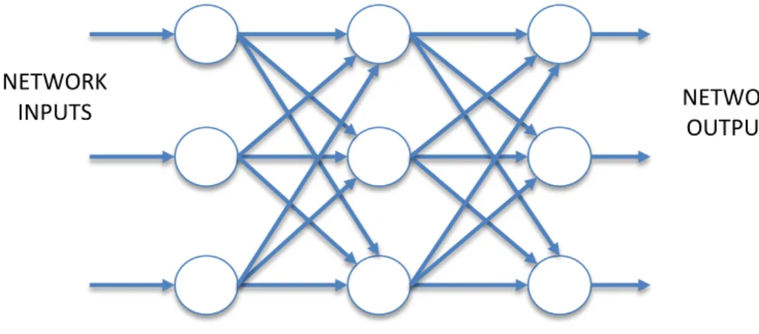
2. Multilayer feed-forward networks – The addition of extra layers to a single layer feed-forward network results in a multilayer feed-forward network. A multilayer feed-forward network contains one or more hidden layers. These hidden layers contain neurons that intervene between the input stimulus and the network output and enable the network to model higher-order statistics (Haykin, 1999). In a multilayer feed-forward network the input layer feeds into the first hidden layer of neurons. This hidden layer undertakes computations and provides an output that is sent to the next hidden layer of neurons. This continues until the output layer is reached where the network provides a final output signal. An example of a multi-layer feed-forward network containing two hidden multi-layers is indicated in
Figure 8 Typical 3-layer fully connected feed-forward ANN.
3. Recurrent networks – Recurrent networks differ from feed-forward networks in that they contain at least one feedback loop.
Figure 8 Typical 3-layer fully connected feed-forward ANN shows a three
20 Chapter 2: Neural Network Primer the diagram, raw data is input into the first layer of the network. Each processing element processes the input information and produces an output. This output is then used as input for each of the processing elements in the second layer. Each of the processing elements in the second layer then process this input information and then computes the output. This output is then fed forward into the third layer. The processing elements in the third layer then take these inputs and compute the output which is the final output from the network.
Figure 8 Typical 3-layer fully connected feed-forward ANN
Network learning
Similar to a biological bring, an ANN needs to be trained or taught the correct answer to a problem. This knowledge can then be retained by the network and applied to new data, in order to provide an output. The typical process for this is (Medsker & Liebowitz, 1994):
1. Compute outputs;
2. Compare outputs with desired answers; and, 3. Adjust the weights and repeat the process.
NETWORK INPUTS HIDDEN LAYER NETWORK OUTPUTS OUTPUT LAYER INPUT LAYER
Chapter 2: Neural Network Primer 21 Different learning methods utilised in ANNs can be classified in one of following categories:
1. Supervised learning – in this situation data is used to train the ANN what is the correct response (output) to the input. When a supervised learning paradigm is adopted, the aim of the ANN is to find a set of weights that minimises the error between the correct result and the computed result. 2. Unsupervised learning – in this situation data is not used to train the ANN.
When this paradigm is adopted, the ANN must determine its own response to the input.
Another type of learning, reinforcement learning, lies somewhere between supervised and unsupervised learning. In this paradigm, the ANN determines its own response to the input (similar to unsupervised learning) but then rates this response as either good (rewarding) or bad (punishable) by comparing its response to the target response. Using this paradigm, the weights are adjusted until an equilibrium state occurs. This type of learning is analogous to the way stimulus and response learning (operant conditioning) occurs in biological creatures (Rao & Srinivas, 2003).
Error Functions
Once the neuron has received and calculated the strength of its input stimulus (i.e. its activation) and then used this activation level to determine its output (using its transformation function) the next step is to determine how accurate the output of the neuron is compared to the target output. Therefore some kind of error function is required.
Typical error functions used include:
• Mean Absolute Error – Network performance is measured as the mean of
22 Chapter 2: Neural Network Primer
• Mean Squared Error /Root Mean Squared Error – Network performance is
measured as the mean of squared errors. In the case of root mean squared error the square root of the mean squared error is used to provide error which has the same units as the output.
• Sum Squared Error - Network performance is measured as the sum of squared errors.
Generally, the network training process occurs until either of the following events occurs:
• A pre-defined, arbitrary error level has been achieved. Once this error level has been achieved, training terminates and simulation can occur.
• The maximum number of calculations (epochs) has been reached.
Back Propagation
Back propagation is a widely used form of supervised learning. It is generally used in a feed forward network structure (hence creating the feed-forward back propagation network). An artificial neural network created to utilise back propagation must have a minimum of three layers (input layer, output layer and at least one hidden layer). The information travels only in the forward direction and there can be no feedback loops (so this type of learning process cannot be applied to recurrent networks). This type of network learns by back propagating the errors during the training phase. The back propagation algorithm changes the neuron input weights to improve accuracy of the network.
The standard method of back propagation relies on the delta rule which is a gradient descent learning rule used to update weights applied to network processing elements. The back propagation algorithm was originally discovered by Werbos
Chapter 2: Neural Network Primer 23 (1974) however, its significance was not realised until later (Patterson, 1995; Rao & Srinivas, 2003). The delta rule provides a method of calculating the gradient of the error function efficiently by using the chain rule of differentiation (Rao & Srinivas, 2003).
The back propagation algorithm functions as follows: 1. Input weights are randomly applied to the network.
2. The network calculations occur and the network produces an output based upon the neuron inputs, the input weights, and the transformation functions.
3. The calculated output is then compared to the target output.
4. The error of the output is calculated using the selected error function. 5. The error is then back propagated through the network, thereby changing
the input weights in each layer.
6. The process (steps 2 – 5) then repeats until the error reaches the desired level or the maximum number of epochs is reached.
The derivation of the back propagation algorithm will be demonstrated logically and confirmed mathematically. Consider the following simple multi-layered feed-forward network:
24 Chapter 2: Neural Network Primer Figure 9 Multi-layer feed-forward network
In this network there are three inputs (x1, x2, x3). The network has three layers.
The input layer has 3 nodes. The hidden layer has three nodes. The output layer has two nodes. Each node in the network is connected to each node in the adjoining layer. The network is feed forward only. This network is classified as a feed-forward network. The output from each node is denoted z. The network is initialised by
applying randomised weightings to each of the node connections and the first training vector is presented to the network for calculation.
Next, the output from each of the input layers is calculated. The output from nodes 1-3 is given by the following equations.
𝑧1 =𝑓(𝑥1) (11)
𝑧2 = 𝑓(𝑥2)
𝑧3 =𝑓(𝑥3)
The function f(x) must be a bounded, differentiable function otherwise the
gradient descent algorithm cannot be utilised.
The output from the hidden layer is then calculated. The output from each of the hidden layers is then calculated using the following formulas:
w58 w57 w68 z6 z4 z5 z2 z3 z1 w48 w67 w47 f1(x) x1 x2 x3 z7 z8 f2(x) f3(x) f4(x) f5(x) f6(x) f7(x) f8(x) Input
Layer Hidden Layer Output Layer
w15 w35 w16 w26 w36 w25 w34 w24 w1
Chapter 2: Neural Network Primer 25
𝑧4 = 𝑓(𝑧1𝑤14+ 𝑧2𝑤24+𝑧3𝑤34) (12)
𝑧5 = 𝑓(𝑧1𝑤15+ 𝑧2𝑤25+𝑧3𝑤35)
𝑧6 = 𝑓(𝑧1𝑤16+ 𝑧2𝑤26+𝑧3𝑤36)
Then the output from the output layer is calculated using the formulas below:
𝑧7 =𝑓(𝑧4𝑤47+ 𝑧5𝑤57+𝑧6𝑤67) (13)
𝑧8 = 𝑓(𝑧4𝑤47+ 𝑧5𝑤57+𝑧6𝑤67)
Now that the output neuron outputs have been calculated, the results need to be compared with the desired results. For the purposes of this derivation and the following proof, mean squared error will be the error measure used. If the desired results from node 7 and 8 are denoted by y then system error is given by:
𝐸 = 𝑛 �1 (𝑦 − 𝑧)2 (14) Error in each node (denoted δ) is then back propagated through the system. Error in the output layer nodes is directly calculated using the formulas below:
𝛿7 = 𝑦7 − 𝑧7 (15)
𝛿8 = 𝑦8− 𝑧8
The amount of error attributable to each node in the hidden layer is dependent on the error in the output layer and the weights between the nodes. The error attributable to each of the hidden layer nodes can be calculated using the following formulas:
𝛿4 =𝑤47𝛿7+ 𝑤48𝛿8 (16)
𝛿5 = 𝑤57𝛿7+ 𝑤58𝛿8
𝛿6 = 𝑤67𝛿7+ 𝑤68𝛿8
Now that errors in the hidden row have been calculated, error attributable to input nodes can be calculated in a similar manner using the formulas below:
𝛿1 = 𝑤14𝛿4+ 𝑤15𝛿5+ 𝑤16𝛿6 (17)
𝛿2 =𝑤24𝛿4+ 𝑤25𝛿5+ 𝑤26𝛿6
26 Chapter 2: Neural Network Primer Now that error signals have been determined for all nodes in the network, the revised weights can be calculated. The new weight is dependent on (1) a scaling factor called the learning rate, (2) the error term calculated for the node, (3) the gradient of the transformation function in the node, (4) the input value. The weight update is given by the following formulas:
𝑤′14 = 𝑤14+ 𝜂𝛿4𝑓′4(𝑥)𝑧1 (18) 𝑤′ 24= 𝑤24+ 𝜂𝛿4𝑓′4(𝑥)𝑧2 𝑤′ 34= 𝑤34+ 𝜂𝛿4𝑓′4(𝑥)𝑧3 𝑤′ 15= 𝑤15+ 𝜂𝛿5𝑓′5(𝑥)𝑧1 𝑤′ 25= 𝑤25+ 𝜂𝛿5𝑓′5(𝑥)𝑧2 𝑤′ 35= 𝑤35+ 𝜂𝛿5𝑓′5(𝑥)𝑧3 𝑤′ 16= 𝑤16+ 𝜂𝛿6𝑓′6(𝑥)𝑧1 𝑤′ 26= 𝑤26+ 𝜂𝛿6𝑓′6(𝑥)𝑧2 𝑤′ 36= 𝑤36+ 𝜂𝛿6𝑓′6(𝑥)𝑧3 𝑤′ 47= 𝑤47+ 𝜂𝛿7𝑓′7(𝑥)𝑧4 𝑤′ 57= 𝑤57+ 𝜂𝛿7𝑓′7(𝑥)𝑧5 𝑤′ 67= 𝑤67+ 𝜂𝛿7𝑓′7(𝑥)𝑧6 𝑤′ 48= 𝑤48+ 𝜂𝛿8𝑓′8(𝑥)𝑧4 𝑤′ 58= 𝑤58+ 𝜂𝛿8𝑓′8(𝑥)𝑧5 𝑤′68= 𝑤68+ 𝜂𝛿8𝑓′8(𝑥)𝑧6
A single iteration (epoch) has now been completed. A new training vector is then presented to the network for output calculation and the procedure continues to repeat until the system error reaches some arbitrary level. The update formulas provided above can be confirmed mathematically. In order to reduce the system error with each successive iteration, the system weights are adjusted in proportion to the negative of the error gradient (Patterson, 1995). Applying this for instance to node 4, then the input weights (w14, w24, w34) should be updated by the negative of the gradient of the error term 𝛿4. Therefore the change in the input weight is given by the formula:
Chapter 2: Neural Network Primer 27 Applying this to node for the following is obtained:
∆𝑤14= −𝜂𝜕𝑤𝜕𝐸 (20) Using the chain rule of differentiation:
𝜕𝐸 𝜕𝑤 = 𝜕𝐸 𝜕𝑥4 𝜕𝑥4 𝜕𝑤 (21) 𝜕𝐸 𝜕𝑤= 𝜕𝐸 𝜕𝑥4 𝜕(𝑧1𝑤14+ 𝑧2𝑤24+𝑧3𝑤34) 𝜕𝑤 (22)
Or stated for specifically for w14:
𝜕𝐸 𝜕𝑤14 = 𝜕𝐸 𝜕𝑥4 𝜕(𝑧1𝑤14+ 𝑧2𝑤24+𝑧3𝑤34) 𝜕𝑤14 (23) 𝜕𝐸 𝜕𝑤14= 𝜕𝐸 𝜕𝑥4 𝑧1 (24)
Again using the chain rule of differentiation:
𝜕𝐸 𝜕𝑤14= 𝜕𝐸 𝜕𝑧4 𝜕𝑧4 𝜕𝑥4𝑧1 (25) Substituting 𝑧4 = 𝑓4(𝑥) so: 𝜕𝐸 𝜕𝑤14= 𝜕𝐸 𝜕𝑧4 𝜕𝑓4(𝑥) 𝜕𝑥4 𝑧1 (26) 𝜕𝐸 𝜕𝑤14= 𝜕𝐸 𝜕𝑧4 𝑓4 ′(𝑥) 𝑧 1 (27)
Substituting for E gives:
𝜕𝐸 𝜕𝑤14= 𝜕12∑(𝑦 − 𝑧)2 𝜕𝑧4 𝑓4 ′(𝑥) 𝑧 1 (28)
28 Chapter 2: Neural Network Primer The factor of ½ has been included for convenience as this will simplify the final result once differentiation has occurred.
𝜕𝐸
𝜕𝑤14 = (𝑦 − 𝑧) 𝑓4
′(𝑥) 𝑧
1 (29)
Restating this formula in generalised terms and inserting the learning rate scaling factor (η) applicable to all nodes and inserting the learning rate constant gives the following formula:
𝑤′𝑖𝑗 = 𝑤𝑖𝑗 + 𝜂𝛿𝑗𝑓′𝑗(𝑥)𝑧𝑖 (30) Network architecture
There are several different artificial neural network topologies. The topology selected determines how the ANN computations take place as has been identified as an important part of ANN development (Mehrotra et al., 1997). There are several
ways in which ANN topologies can be classified. Firstly ANNs can be classified according to connectivity. A fully connected ANN is an ANN where every neuron is connected to every other neuron. The connections are all weighted and therefore can be excitatory or inhibitory. This is the most general type of ANN and all other ANN structures can be considered a special case whereby some connection weights are fixed to zero (w = 0).
The other main distinction that can be drawn is between:
• Feed forward networks
• Recurrent networks
A feed forward network is a network where signals are allowed to travel forward only. The network may contain several layers of processing elements. There is no feedback (i.e. no connections extending from outputs of processing elements in
Chapter 2: Neural Network Primer 29 one layer into inputs of processing elements in the same or previous layers). Conversely a recurrent network has signals that travel in both directions. This feedback is created by having connections extending from outputs of processing elements in one layer into inputs of processing elements in the same or previous layer.
30 Chapter 3: Literature review
Chapter 3:
Literature review
Why use artificial neural networks
There are alternatives to using ANNs for stock price prediction and portfolio selection. While the theoretical and computational basis for ANNs and multiple regressions models is significantly different, each of these techniques can be used to predict the relationship between several independent, predictor variables and a dependent variable (in this case the quantum of price movement). Given how relatively complex the ANN approach is compared to a multiple regression model, it is worth considering the limitations of regression analyses and the benefits achieved by using ANNs. Of prime importance is the observation that comparative studies have shown that ANNs consistently outperform regression models where input data contains nonlinearities (Comrie, 1997).
Multiple regression is a linear model that assumes that the relationship between a set of independent, predictor variables and a dependent variable is linear but there is some noise affecting the linear relationship. A procedure is then used to determine what the regression coefficients are that minimise the system error. Typically ordinary least squares, or generalised least squares is used. Ordinary least squares is the simplest and most efficient method which minimises the sum of the squared error in each measurement. The generalised least squares method is an extension of the ordinary least squares method which allows for heteroscedasticity or correlations between error terms in the model.
The assumption of linearity is key to accuracy in multiple regression model prediction. If the relationship is not linear, then the regression analysis will under
Chapter 3: Literature review 31 estimate the true relationship. This under estimate in turn carries two risks (Osborne & Waters, 2002)–
1. Increased probability of Type II error (failing to reject the null hypothesis when it is actually false) for each independent variable for which this assumption does not hold.
2. Increased probability of Type I error (incorrectly rejecting the null hypothesis) for other independent variables that share variance with that independent variable.
Multiple regression is also a Gaussian technique of analysis which assumes that variables have normal distributions. This assumption can mean that the model is not robust to situations where variables have fat tailed distributions such a Power law or Mandlebrotian distributions that are often encountered in the financial domain. These fat tailed, outlying data points can distort relationships and significance tests (Osborne & Waters, 2002).
Regression models also assume homoscedasticity which means that the variance of errors is constant over the range of values for an independent variable. Slight heteroscedasticity has been shown to have little effect on significant tests (Tabachnick & Fidell, 1996) however at higher levels heteroscedasticity can significantly increase the possibility of a Type I (failing to reject the null hypothesis when it is actually false) error (Osborne & Waters, 2002). These limitations of multiple regression provide a powerful basis for using ANNs. ANNs in contrast can be formulated to be non-parametric, making no assumptions about the independent variables, the dependent variable or the error. It is therefore reasonable to assert that theoretically ANNs could outperform multiple regression models to predict future equity prices.
32 Chapter 3: Literature review Neural networks in finance research
The body of research in the field has been steadily growing over the past twenty years. The following discussion focuses on some of the relevant research in the field.
Yoon and Swales (1991) used ANNs to examine stock price performance with US stocks and compared the results obtained using the ANN technique against using a multiple discriminant analysis approach. The researchers created two data sets. The first data set comprised 58 companies which had the highest total returns in each year selected from Fortune 500 firms divided into five industries. The second data set of 40 firms was selected from 10 industries reported by Business Week to have the highest valuations. For each company included in the study the researchers undertook content analysis to analyse the president’s letter to stockholders contained in the annual report. The frequency data set created by the content analysis was then used for both the multiple discriminant analysis technique and the ANN technique to predict stock price performance.
The ANN created by Yoon and Swales (1991) was a four-layered network. The input layer contained 9 variables:
• Confidence • Economic factor • Growth • Strategic plans • New products • Anticipated losses
Chapter 3: Literature review 33
• Anticipated gains
• Long-term optimism
• Short-term optimism
These inputs were fed into the first hidden layer which contained 3 neurons. The output of the first hidden layer of neurons was then fed into the second hidden layer and the output layer. The ANN output for each stock was a classification as either a firm whose stock price performed well or a firm whose stock price performed poorly. The analysis indicated that the ANN technique significantly outperformed the multiple discriminant analysis technique to predict stock price performance (Yoon & Swales, 1991). The researchers also noted that the number of hidden neurons included in the network contributed to its viability and that more units resulted in better performance up to a point only, after which adding further hidden units impaired the model’s performance (Yoon & Swales, 1991).
Kryzanowski et al. (1992) used ANNs to pick stocks. Their study relied on a
particular type of ANN called a Boltzmann Machine which is a type of stochastic recurrent neural network. The researchers used fundamental data available from the annual financial statements for 120 publicly traded companies over a six year period from 1984-1989. For each company, the trends of fourteen different financial ratios were examined:
• Gross profit margin*
• Net profit margin*
• Total asset turnover • Fixed asset turnover
34 Chapter 3: Literature review
• Return on total assets
• Return on equity*
• Debt ratio
• Debt to equity ratio* • Interest coverage ratio
• Long term debt ratio
• Current ratio*
• Quick ratio
• Accounts receivable turnover
• Accounts payable turnover
Five of these ratios (marked “*”) were then benchmarked against industry averages. Rather than using the actual ratios above as input into the ANN the researchers coded each of the ratios (i.e. each of the input parameters was coded as trending either downward, upward or neutral).
The study found that the Boltzmann Machine achieved accuracy of 66% in accurately predicting a stock’s directional movement over the subsequent year (Kryzanowski et al., 1992). This result was achieved using a network that created a
binary output. In additional, Kryzanowski et al. re-tested the network with a
three-state output option. This allowed the neural network to give a stock a neutral classification where it could not make a clear decision on directional movement. When allowed to utilise a three-category output the accuracy of the ANN increased to over 71%.
Chapter 3: Literature review 35 One problem identified was the failure of the Boltzmann Machine to accurately predict extreme price movements. For example, the ANN predicted a negative return for a stock which increased in price 150% and similarly predicted a positive return for a stock which lost 73%. This has substantial implications for the design of the ANN and the trading scheme utilised. It is possible that the usual measures for accuracy of ANNs such as root mean square error might not be optimal. For example, it may be easier to obtain abnormal returns by having an ANN which correctly predicts extreme price movements but cannot accurately predict small stock price movements. It is also worth noting that this research utilised a relatively short testing period of three years.
ANNs have also been utilised for portfolio selection with American stocks. The Pension and Investment Department of Deere & Company used an ANN to create a style-based stock portfolio. The objective of the ANN was to (Hall, 1994):
1. Identify the style of stocks with the largest recent price increases and apply this style to the current market to select a portfolio intended to outperform the S&P Index in the short term;
2. Provide buy and sell signals; and,
3. Automatically and continuously learn to adapt to changing market conditions.
The ANN created consisted of several weeks of historical data for the 1,000 largest US corporations listed on the S&P. Each data point in the set contained 37 pre-processed input variables and a single output (predicted change in stock price) (Hall, 1994). The stocks were then ranked according to predicted performance. The portfolio was managed using a simple strategy:
1. Sell stocks in the portfolio when its ranking falls below a predetermined threshold for a given period of time.
36 Chapter 3: Literature review 2. Replace any stocks sold with the highest ranking stocks not currently in
the portfolio.
The portfolio commenced with a value of $100 million. The portfolio contained 80 equally weighted stocks. While the author indicates that the performance of the portfolio after transactions costs has exceeded the S&P 500 since inception, disappointingly, actual performance results and specific details of the system were not published, citing the proprietary nature of the results (Hall, 1994). While this research suggests the viability of ANNs for portfolio selection, there is insufficient detail to critically evaluate the research. The authors of the study did provide some guidelines for the creation of evolutionary complex systems to manage stock portfolios (Hall, 1994):
1. Be willing to trade short-term accuracy for long-term performance:
Even with the processing power of modern computers and the complexity of ANNs, it is not realistic to expect more than rough estimates from the models. The authors note that even rough estimates can be used to achieve significant excess returns. The researchers conclude that when dealing with complex evolutionary systems, the accuracy of a model in explaining some local condition is inversely proportional to its usefulness in discovering and explaining future states.
In practice this means that fewer degrees of freedom often lead to better predictive performance. This means that the system inputs need to be carefully selected. Pre-processing of these inputs can reduce the number of inputs required and the number of degrees of freedom required to achieve a high level of predictive capability.
Chapter 3: Literature review 37 2. Select the proper modelling tool:
Hall notes that selecting the correct modelling tool is of primary importance. For example when linear regression models are used the number of degrees of freedom is fixed depending on the model, and is always higher than the number of system inputs. This is quite different to ANNs which can be constructed so that they have many potential inputs but few degrees of freedom. This characteristic of ANNs is significant in portfolio selection.
3. Discover the proper predictive period of the system:
Long term predictions using complex evolutionary systems are unreliable due to uncontrollable external events. Short term predictions are unreliable due to the significant amount of noise inherent in the data. However, Hall identifies that there is some period into the future for which useful predictions can be made and that discovering this predictive period of the system is a critical task in modelling.
Hall suggests that the predictive period will be affected by many factors including the accuracy of the model, the characteristics of the trading system attached to the model, the amount of noise in the data, and the underlying dynamics of the problem.
4. Select a sampling rate for the training data that is compatible with the prediction period:
After the predictive period has been determined, the training data for the ANN needs to be selected. Hall suggests that the sampling rate of the training data must be compatible with the time period of the model prediction. For example, it would not make sense to try to train an ANN to predict weekly changes in stock price with 30 minutes of price data, sampled at one minute intervals. Hall suggests a heuristic that the sampling period of the data used to train the ANN should be 0.1 to 0.5 of the