Vol 7, No 8 (2017)

(1)

Research Article

a

August

2017

Computer Science and Software Engineering

ISSN: 2277-128X (Volume-7, Issue-8)

Performance Analysis of TBC-ACO Routing Protocol with

Existing Routing Protocols of Wireless Sensor Networks

A. Radhika

Ph.D (CSE) Research Scholar, Rayalaseema University, Kurnool, Andhra Pradesh, India

Dr. D. Haritha

HOD (CSE) SRK Institute of Technology, Vijayawada, Andhra Pradesh, India

DOI: 10.23956/ijarcsse/V7I8/0104

Abstract— Wireless Sensor Networks, have witnessed significant amount of improvement in research across various areas like Routing, Security, Localization, Deployment and above all Energy Efficiency. Congestion is a problem of importance in resource constrained Wireless Sensor Networks, especially for large networks, where the traffic loads exceed the available capacity of the resources . Sensor nodes are prone to failure and the misbehaviour of these faulty nodes creates further congestion. The resulting effect is a degradation in network performance, additional computation and increased energy consumption, which in turn decreases network lifetime. Hence, the data packet routing algorithm should consider congestion as one of the parameters, in addition to the role of the faulty nodes and not merely energy efficient protocols .Nowadays, the main central point of attraction is the concept of Swarm Intelligence based techniques integration in WSN. Swarm Intelligence based Computational Swarm Intelligence Techniques have improvised WSN in terms of efficiency, Performance, robustness and scalability. The main objective of this research paper is to propose congestion aware , energy efficient, routing approach that utilizes Ant Colony Optimization, in which faulty nodes are isolated by means of the concept of trust further we compare the performance of various existing routing protocols like AODV, DSDV and DSR routing protocols, ACO Based Routing Protocol with Trust Based Congestion aware ACO Based Routing in terms of End to End Delay, Packet Delivery Rate, Routing Overhead, Throughput and Energy Efficiency. Simulation based results and data analysis shows that overall TBC-ACO is 150% more efficient in terms of overall performance as compared to other existing routing protocols for Wireless Sensor Networks.

Keywords— Wireless Sensor Networks, Swarm Intelligence, Ant Colony Optimization (ACO), AODV, DSDV, DSR, Trust Based Congestion-ACO, Performance.

I. INTRODUCTION

(2)

ISSN(E): 2277-128X, ISSN(P): 2277-6451, DOI: 10.23956/ijarcsse/V7I8/0104, pp. 169-180

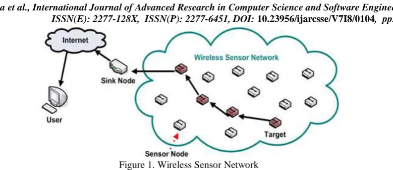
Figure 1. Wireless Sensor Network

II. SWARM INTELLIGENCE

Swarm Intelligence [6-9], another novel branch of Artificial Intelligence, has attracted several researchers to apply SI based optimization techniques in solving varied problems of Robotics, Networking, Wireless Communications, Drones, Electronics, Information Theory and other diverse areas. Swarm Intelligence concept was first introduced by Gerardo Beni and Jing Wang [10] in 1989 with relation to cellular robotic systems. In general terms, Swarm Intelligence is modelling of collective behaviors of simple agents interacting locally among themselves, and their environment, which leads to the evolution of a coherent functional global pattern. These models are inspired by social behavior of insects and other animals. Talking in terms of computation, Swarm Intelligence models are computing algorithm models used for undertaking and solving complex distributed optimization problems. In Swam Intelligence, the most significant concept is ―Swarm‖. Swarm is used to refer any restrained collection of interacting agents or individuals. Communication among these swarms in distributed manner without any requirement of centralized control mechanism makes these models highly realistic and robust to be implemented in diverse applications. The concept of Swarm Intelligence was started by two main Algorithms: Ant Colony Optimization (ACO) being developed by Dorigo and Stutzle in 2004 and Particle Swarm Optimization (PSO) being developed by Kennedy and Elberhart in 2001. With time, various other algorithms have come up and make the Swarm Intelligence more rich and implementable in different applications like Fish Swarm, Monkey Swarm, Glow worms, Bee Colony, Artificial Immune System, Firefly Algorithm and many more. Swarm Intelligence primarily works on two founding principles: 1. Self Organization 2. Stigmergy Self-Organization: The concept of Self Organization was defined by Bonabeau et al [11,12] in 1999 as ―Self Organization is a set of Dynamic Mechanisms whereby structures appear at the global level of a system from interactions of its lower-level components”. Self organization lays the foundation of three important characteristics: Structure, Multi-Stability and State Transition.Structure: It is founded from a homogeneous start-up state. E.g. Ant Foraging trails. Multi-Stability: Co-existence of many stable states. E.g.Behavior of ants to search for food random in field. State Transitions: Change of System Behavior. Example: Location of new food source after finishing the entire food transmit from source to nest. Stigmergy:

The word ―Stigmergy‖ is mix of two words: Stigma= Work and Ergon=Work which means Simulation by work. It is based on the principle that the main area to operate for swarms in Environment and work is not dependent on specific agents. It can be summarized as, ―Coordination, Cooperation and Regulation of tasks doesn’t depend on workers directly, but on construction themselves”. The worker is properly guided rather than directed to perform the work. It is also a special form of stimulation called Stigmergy.

Stigmergy can be of following types:

For modelling the behaviors of Swarms, Millonas [13] laid the following 4 Principles as follows:

1. Proximity Principle of Swarm: Swarms should be highly capable to perform simple computations with respect to the environment existing around them in terms of time and space. E.g. Search for living place and building nest in coordination.

2. Quality Principle of Swarm: Swarm should be highly respondent to environmental quality factors like food, safety and other stuff.

3. Diverse Response Principle of Swam: The swarm should not allocate all of its resources along excessively narrow channels and it should distribute resources into many nodes.

4. Stability and Adaptability Principle of Swarm: Swarms are expected to adapt environmental fluctuations without rapidly changing modes since mode changing involves tremendous amounts of energy.

III. ANT COLONY OPTIMIZATION A. Introduction to Ant Colony Optimization

(3)

Ants are highly sophisticated and intelligent swarms to find the shortest path from food source to nest by depositing pheromone on the ground and laying the trails so that other ants can follow. The most important component of ACO Algorithms is the combination of a priori information regarding the structure with a posteriori information about the structure of previously obtained optimal solutions. In order to determine the shortest path, a moving ant lay the pheromone which acts as base for other ants to follow and deciding the high probability to follow it. As a result, it leads to the emergence of collective behavior and forms a positive feedback loop system through which other ants can follow the path and makes the pheromone more stable and best path for transferring the food back to nest.

B. Ant Colony Optimization-Definition

Ant Colony Optimization technique is based on ants i.e. how ant colonies find the efficient path between nest and food source. In search of food, ants roam randomly in the environment. On location of the food source, ant’s first return back to their nest by laying a trail of chemical substance called ―Pheromone‖ in their path. Pheromone lays the foundation for communication medium for other ants to follow the way and go to the food source. When other ants follow the path, the quantity of pheromone increases on that particular path. The rich the quantity of pheromone along the path, the more likely is that other ants will detect and follow the path. In other words, ants follow that path which is marked by strongest pheromone quantity. As pheromone evaporates over time, which in turn reduces its attractive strength. The longer the time taken by ant to travel the path from food source to nest, the quicker the pheromone will evaporate. So, the path should be shorter so that the active strength of pheromone is maintained and ants can easily transfer the food from source to nest. So, in turn of this policy the shortest path will naturally emerge.

Algorithm: Ant Colony Optimization

Initialize Parameters Initialize pheromone trails Create ants

While stopping criteria is not reached, do

Let all ants construct their solution Update pheromone trails

Allow Daemon Actions

End while

C. Suitablilty of Ant Colony Optimization Routing Algorithm towards Wireless Sensor Networks

Ant Colony Optimization Routing Algorithm mentioned above is highly suitable and performs well in Wireless Sensor Networks because of the following reasons:

1) Provide traffic adaptive and multipath routing.

2) Rely on both passive and active information monitoring and gathering. 3) Making use of stochastic components.

4) Don’t allow local estimates to have global impact.

5) Setup paths in a less selfish way than in pure shortest path schemes favoring load balancing. 6) Showing limited sensitivity to parameter settings

D. Basic Ant Routing Algorithm [17]

Let G =(𝑉, 𝐸 ) be a connected graph with n = |𝑉| nodes. The simple ant colony algorithm can be used to find the shortest path between a source node 𝑣𝑠 and a destination node 𝑣𝑑 on the graph G. The path length is given by the number of nodes on the path.Each edge 𝑒 (𝑖, 𝑗)𝜖 of the graph connecting the nodes 𝑣𝑖 and 𝑣𝑗 has a variable 𝜑𝑖,𝑗 (artificial pheromone), which is modified by the ants when they visit the node.

The pheromone concentration 𝜑𝑖, is an indication of the usage of this edge. delay(path(i,j))=∑e€p(i,j) delay(e)+ ∑ n€p(i,j) delay(n)

An ant located in node 𝑣𝑣𝑖𝑖 uses pheromone 𝜑𝑖, of node 𝑣𝑗𝜖𝑁 to compute the probability of node 𝑣𝑗 as next hop. 𝑁 is the set of one-step neighbours of node .

Pi,j = 𝜑ij

if j€Ni

∑i€p(i,j) 𝜑𝑖,𝑗

Pi,j = 0 if j ∉ Ni

The transition probabilities 𝑝𝑖, of a node 𝑣𝑖 full fill the constraint: Σ𝑗∈𝑁𝑖𝑃𝑖= 1, 𝑖∈ [1,N]

In the simple ant colony algorithm, the ants deposit a constant amount of pheromone. An ant changes the amount Δ𝜑 of pheromone of the edge ( , 𝑣𝑗 ) when moving from node 𝑣𝑖 to node 𝑣𝑗 as follows:

𝜑ij ≔𝜑𝑖𝑗 + Δ𝜑

Artificial pheromone concentration decreases with time to inhibit a fast convergence of pheromone on the edges.

E. Basic Ant Colony Routing Algorithm- Working

(4)

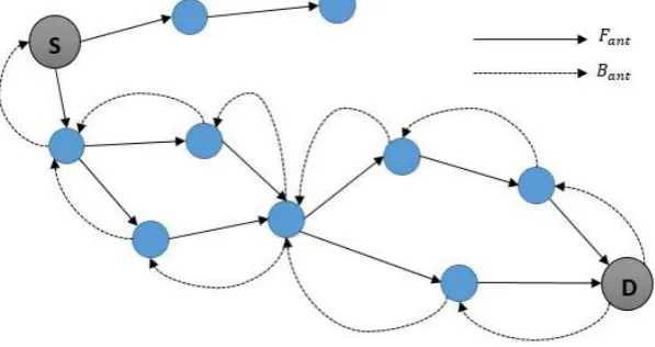
1. Route Discovery : In this phase, the new routes discovery takes place and leads to the creation of a forward ant (𝐹𝑎nt) and a backward ant ( 𝐵𝑎nt). A 𝐹𝑎nt is an agent which establishes the pheromone track to the source node. In contrast, a

𝐵𝑎nt establishes the pheromone track to the destination node. The 𝐹𝑎nt is a small packet with a unique sequence number. Nodes are able to distinguish duplicate packets on basis of the sequence number and the source address of the 𝐹𝑎nt . A forward ant is broadcasted by the sender and will be relayed by the neighbors of the sender A node receiving then 𝐹𝑎nt for the first time, creates a record in its routing table.

Figure 2. Route Discovery Phase in Ant Colony Routing

A record in the routing table is a triple and consists of (destination address, next hop, pheromone value). The node interprets the source address of the 𝐹𝑎nt as destination address, the address of the previous node as the next hop, and computes the pheromone value depending on the number of relays the 𝐹𝑎nt to its neighbours. Duplicate 𝐹𝑎nt is identified

through the unique sequence number and destroyed by the nodes. When the 𝐹𝑎nt reaches the destination node, it is

processed in a special way. The destination node extracts the information of the 𝐹𝑎nt and destroys it. Subsequently, it creates a 𝐵𝑎nt and sends it to the source node. The 𝐵𝑎nt has the same task as the 𝐹𝑎nt, i.e. establishing a track to this node.

When the sender receives the 𝐵𝑎nt from the destination node, the path is established and data packet scan be sent

2. Route Maintenance: After establishing the pheromone levels by Fant and Bant, data packets are used to maintain the routing path.

3. Handling Route Failure The last stage of Basic Ant Routing is Handling Route Failure which is caused by node mobility and occurs in Wireless Sensor Nodes. It recognizes via acknowledgement missing and searches for alternative link to send packet via that path. If the packet sent, doesn’t reach the destination, the source node performs the duty to discover new routing path to transmit the packets.

The following fig.3 elaborates the Workflow of Basic Ant Colony Routing Algorithm as mentioned above in form of flow chart

(5)

ISSN(E): 2277-128X, ISSN(P): 2277-6451, DOI: 10.23956/ijarcsse/V7I8/0104, pp. 169-180 IV. TRUST BASED CONGESTION AWARE ANT COLONY OPTIMIZATION:

In trust based ant colony routing we present a congestion aware energy efficient trusted routing scheme for WSN in which ACO algorithm is utilized to maximize the network lifetime.

A. Stage 1

In stage 1 trust value detects the misbehaviour of sensor nodes.The trust congestion metric is generated for the trusted nodes (also called valid nodes), for the data packet routing algorithm which is implemented in the next stage. The malicious nodes having trust value below the threshold level are not considered for data packet routing,due to which the congestion metric is not computed for such nodes. This causes a reduction in the computation overhead and thereby enhances battery life time.

1) Trust Computation: The trust value of node i upon node j is calculated based on trust metrics namely, remaining node energy (Ne), packet transmission ration (PTR) and packet latency ratio (PL). All the parameters are normalized so that the

values belong to the range: [0,1]. PTR is defined as the ratio of the number of acknowledgement received from node j to

the total number of packets sent from node i to node j. PL is the ratio of the latency(time it takes for the packet to reach

the destination.Nae is defined as the average energy of the node i and node j. if Ei and Ej are the existing energy value of

node i and node j respectively, then

Nae = (Ei + Ej) / 2. The energy of a sensor node should be greater than or equal to the threshold value of Eth for

transmitting data packets to its one hop neighbor in the radio communication range. Trust of node upon node j is calculated by the following equation

Tij = w1*Nae+ W2*PTR+W3*PL

...(1) W1+W2+W3

where w1,w2,w3 are the corresponding weights used for Nae,PTR,PL such that w1,w2,w3 E [0,1]. A

predefined trust threshold value (T TH ) is set on the basis of the application of the sensor networks [18].

If Tij> TTH, the link between the node i and j is called a trustworthy link. Similarly if, Tij < TTH the link is termed as an

untrusted link. The nodes having no trustworthy link are called malicious nodes and those with at least one trusted link are called trusted nodes (valid nodes) that can take part in data packet routing.

2) Estimation of Network Node Congestion: The congestion level of a valid node is estimated with the help of the parameter known as the Congestion Index. Each node maintains a queue for storing data packets in its buffer. As packets are transmitted from a particular node towards the next node, buffer space is cleared and the packets waiting in the queue go to the empty buffer space of the node. When the packet received rate of the node is greater than the packet transmission rate, queue length increases, buffer overflows, congestion level of the node increases. If a node is not able to clear the data packet in its queue, then it waits for a certain number of pre-defined cycles and holds thepackets in each cycle until the packets are finally dropped .

The Congestion Index of the mth node is calculated by the equation CIm = rinm + Qm(n-1) - routm

... (2)

rinm + Qm(n-1)

where Qm(n-1) is the empty space left in the queue of the mth node till (n-1) th cycle .The parameters rinm , routm is defined as

n-1 ∑ (Nin)

i=1

rinm = ... (3)

n-1

n-1 ∑ (Nno)

i=1

rnom = ... (4)

n-1

Nin = Number of packets forwarded to n th

node in ith cycle

Nno =Number of packets forwarded oth nodes to other nodes in ith cycle.

The congestion index of each trusted node, which is calculated by using equation (2), represents the node level congestion of the WSN. It is calculated dynamically at regular intervals, depending upon the application of the network. 3) Computation of Trust based Congestion Metric (TBCM) : The Trust based Congestion Metric (TBCM) of each trusted nodes, also called as the valid node, is computed by the equation:

TBCij = α * CIj * (1- α)Tij ... (5)

where node i and node j are considered as the source node and the destination node, respectively. CIj is the Congestion

Index of the destination node and Tij is the trust value of source node i upon the destination node j. The constant is α

denoted as Trust Congestion Coefficient which belongs to [0,1].

The proposed TC -ACO algorithm stage 2 implements the data routing protocol using Ant Colony Optimization [6] - [8].The probability Pij for transmission of data packets in optimal route from node i in level L to node j in level (L+ 1) is

(6)

PIJ = (TBCij) β1

.(1/dij) β2

.(Ƭij ) β3

... (6)

∑ (TBCik)β1 .(1/dik)β2 .(Ƭik ) β3

Ұk

where' k' represents all the valid nodes in level (L+ 1). We consider random deployment of sensor nodes in the entire sensor field at the various levels as depicted in Fig. 1, denoted by level 0, 1, 2 . . . Ievel L, (L+l) . . . . level (r-l), level r respectively. The source node is considered as a level 0 node.All nodes within the one hop neighbor of the source node in the radio communication range are denoted as the level 1 nodes. Similarly, all nodes within the one hop neighbor of the level 1 in the radio communication range are called the level 2 nodes and so on. At the end of the cycle c, Ƭij is updated

Ƭij =(1-ρ). Ƭij(n-1)+ Nij/dij ... (7)

The data packet routing algorithm used in the proposed TBC-ACO as For each node i in the Lth level

do

Step1: Find all the valid node k in level (L+1).The node satisfying the condition Tij>TTH are valid nodes

Step 2: Compute the probability of packet transmission from node i to node j defined as Pij

Step 3: Arrange the nodes in descending order based on value of pij and store in the matrix

Step4:Initialize p=1

while (Ei>=Eth) && p<=size(x))

if (Queue(x(p)th node is full OR Ex(p) <ETH))

p=p+1 end if end while end do END

Number of Rounds

protocols Percentage of Dead Nodes

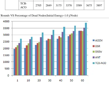
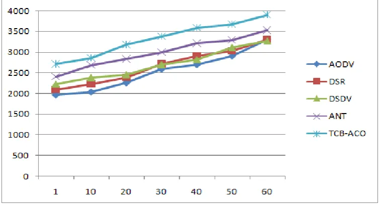
1 10 20 30 40 50 60 AODV 1965 2032 2252 2586 2701 2908 3298 DSR 2086 2222 2390 2704 2896 3029 3308 DSDV 2231 2375 2457 2689 2816 3107 3275 ANT 2404 2677 2828 2994 3209 3284 3522

TCB-ACO 2705 2849 3175 3378 3589 3675 3897

Number of Rounds VS Percentage of Dead Nodes(Initial Energy=1.0 j/Node)

(7)

Fig. 5. Performance Analysis of the Protocols with Initial Energy 1.0 J/Node

V. COMPARISON OF TBC-ACO ROUTING PROTOCOL WITH EXISTING ROUTING PROTOCOLS OF WIRELESS SENSOR NETWORKS

In this part, trust based congestion aware Ant Colony Optimization Routing Protocol is compared with existing protocols of Wireless Sensor Networks. In order to prove the improvement in Routing provided by ACO based routing protocol, the results are compared with AODV [19], DSDV [20] and DSR Routing [21] and Antnet protocol on the basis of Probability of Packet Delivery Rate, Throughput, Routing Overhead, Energy Consumption,End-to-End Delay. Metrics used for Simulation:

1. Packet Delivery Rate : It is the measure of the percentage of packets delivered successfully to the target nodes. Packet Delivery Ratio: (No. of Packets Sent – Packet Loss)* 100/no. of packets sent.

Overhead is determined on the above mentioned Simulation Scenario on varied time intervals

Introduction

Packet Delivery Overhead is determined on the above mentioned Simulation Scenario on varied time intervals and Data values generated under varied Simulation scenarios are as follows

SimulationTime Probability of packet Delivery rate

(8)

Figure 6. Performance Comparison of Routing Protocols on basis of Packet Delivery Ratio

Analysis show significant improvement by ACO in Packet Delivery which is near to about 90% as compared to other existing protocols for wireless sensor networks.

2. Throughput: Throughput is the amount of digital data per time unit delivered over a physical or logical link. It is measured in bits per second, occasionally in data packets per second or data packets per time slot.

Throughput = Number of packets send successfully / total time

Throughput is determined on the above mentioned Simulation Scenario and Data values generated at varied Simulation Time intervals are as follows:

Simulation Time

Throughtput(Mbps)

DSDV AODV DSR ACO TBC-ACO 100 6.335 7.893 8.021 8.547 9.5876 200 7.123 7.675 8.234 9.234 10.234 300 8.342 8.435 8.831 9.235 11.325 400 8.932 9.346 9.0234 9.843 11.634 500 9.234 9.892 9.673 10.234 12.782 600 9.834 9.734 9.543 10.567 12.112

(9)

Analysis shows significant improvement in terms of Network Throughput maintained by ACO Routing Protocol in entire network as compared to other protocols in Sensor networks scenarios.

3. Routing Overhead: Routing Overhead is the number of routing packets required for network communication. Routing Overhead is determined via awk scripts which processes the trace file and gives the result output.

Values:

Routing Overhead(%)

DSDV AODV DSR ACO TBC-ACO 25 9.541234 7.24432 5.039923 5.42321 5.02451 50 7.43252 6.193492 6.702356 5.290234 4.89101 75 6.336234 6.116734 7.432561 6.345781 4.672345 100 9.864532 6.432151 7.743215 5.512341 4.345189 125 6.160234 8.256178 0.714981 5.623167 4.217894 150 9.323567 8.943521 6.632145 6.33216 4.012368

Figure 8.Performance Comparison of Routing Protocols on basis of Routing Overhead

Analysis shows less amount of Routing overhead atleast 70% less amount of routing overhead is being determined in case of TBC-ACO as compared to ACO,DSDV, DSR and AODV routing protocol in sensor network scenarios.

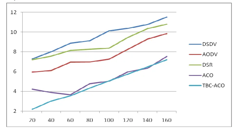
4. End to End Delay: End-To-End delay refers to the time taken for a packet to be transmitted across a network from source to destination. Data transmission seldom occurs only between two adjacent nodes, but via a path which may include many intermediate nodes.

End-to-End delay is the sum of delays experienced at each hop from source to destination. End-To-End Delay = Time Spend on Hop 1 + Time Spendon Hop 2 + …+ Time Spend on Hop n.

End to End Delay is determined on the above mentioned Simulation Scenario and Data values generated at varied time intervals are as follows:

End to End Delay(ms)

(10)

End-To-End delay

Figure 9.Performance Comparison of Routing Protocols on basis of End-To-End delay

5. Energy Consumption: Energy Consumption is termed as the power utilized by sensor nodes in network for transmission of data packets. In this scenario, we have analyzed the energy efficiency of routing protocols in WSN and compared with TBC-ACO to see the efficiency in energy conservation.

Number of Nodes

Energy Consumption in %

DSDV AODV DSR ACO TBC-ACO

25 98.21 98.2 99.42 99.52 99.88 50 97.36 97.56 98.45 98.31 98.56

75 88.25 95.89 94.65 95.46 96.45

100 85.08 89.87 90.32 91.48 94.34 125 81.176 86.38 87.45 89.09 90.23

150 77.405 82.76 84.301 86.3 88.73 175 73.436 79.23 81.012 84.78 86.44

200 72.459 75.72 77.723 80.98 85.23

(11)

Analysis show that as compared to other routing protocols, ACO used almost 120% less amount of energy of sensor nodes for transmitting data among other nodes.

VI. CONCLUSIONS AND FUTURE SCOPE

Wireless Sensor Networks are regarded as highly dynamic, flexible and special type of networks which are gaining researchers attention in recent times. Wireless Sensor Networks are using multi-path routing instead of static networks infrastructure and are always making use of Dynamic topology in real-world implementations. Therefore,there are always new challenges are shortcomings in routing protocols of WSNs as traditional protocols are not getting replaced by latest protocols based on Swarm Intelligence based techniques like ACO, BEE Colony or PSO. Researchers are designing new protocols and are comparing the protocols with existing protocols in terms of suitability, stability and performance. This research paper is a novel attempt towards comprehensive evaluation of five main protocols- AODV,DSDV, DSR and ACO Based Routing Protocol, Trust Based Congestion-ACO Routing Protocol. In the past few years, new standards are implemented to enhance the performance of sensor nodes operating in WSN environment. In this paper, using the latest simulation environment NS-2.35, we have evaluated performance of five routing protocols on basis of Packet Delivery Rate, Throughput, End to End Delay, Routing Overhead and Energy Efficiency and the Data Values and Graphical Analysis shows that SI based TBC-ACO Routing Protocol overrun’s in terms of various parameters and further improves the overall performance of WSN network in real-world environments. In short, TBC-ACO Routing Protocol is all round performer as it has low end-to-end delay, less packet overhead, best throughput, less routing overhead and maintains energy efficiency in the network.

REFERENCES

[1] Rawat, P., Singh, K. D., Chaouchi, H., & Bonnin, J. M. (2014). Wireless sensor networks: a survey on recent developments and potential synergies. The Journal of supercomputing, 68(1), 1-48.

[2] Kulkarni, R. V., Forster, A., & Venayagamoorthy, G. K. (2011). Computational intelligence in wireless sensor networks: A survey. IEEE communications surveys & tutorials, 13(1), 68-96.

[3] Potdar, V., Sharif, A., & Chang, E. (2009, May). Wireless sensor networks: A survey. In Advanced Information Networking and Applications Workshops, 2009. WAINA'09. International Conference on (pp. 636-641). IEEE. [4] Akyildiz, I. F., & Vuran, M. C. (2010). Wireless sensor networks (Vol. 4). John Wiley & Sons.

[5] Yick, J., Mukherjee, B., & Ghosal, D. (2008). Wireless sensor network survey. Computer networks, 52(12), 2292-2330

[6] Blum, C., & Li, X. (2008). Swarm intelligence in optimization. In Swarm Intelligence (pp. 43-85). Springer Berlin Heidelberg.

[7] Dorigo, M., Birattari, M., Blum, C., Clerc, M., Stützle, T., & Winfield, A. (Eds.). (2008). Ant Colo ny Optimization and Swarm Intelligence: 6th International Conference, ANTS 2008, Brussels, Belgium, September 22-24, 2008, Proceedings (Vol. 5217). Springer.

[8] Bonabeau, E., Dorigo, M., & Theraulaz, G. (1999). Swarm intelligence: from natural to artificial systems (No. 1). Oxford university press.

[9] Dorigo, M., & Birattari, M. (2007). Swarm intelligence

[10] Beni, G., & Wang, J. (1993). Swarm intelligence in cellular robotic systems. In Robots and Biological Systems: Towardsa New Bionics? (pp. 703-712). Springer Berlin Heidelberg.

[11] Bonabeau, E., Theraulaz, G., Deneubourg, J. L., Aron, S., & Camazine, S. (1997). Self-organization in social insects.Trends in Ecology & Evolution, 12(5), 188-193.

[12] Bonabeau, E., Theraulaz, G., & Deneubourg, J. L. (1999).Dominance orders in animal societies: the self-organization hypothesis revisited. Bulletin of mathematical biology, 61(4),727-757.

[13] Millonas, M. M., & Dykman, M. I. (1994). Transport and current reversal in stochastically driven ratchets. Physics Letters A, 185(1), 65-69.

[14] Dorigo, M., Maniezzo, V., & Colorni, A. (1996). Ant system:optimization by a colony of cooperating agents. IEEE Transactions on Systems, Man, and Cybernetics, Part B (Cybernetics), 26(1), 29-41.

[15] Dorigo, M., & Gambardella, L. M. (1997). Ant colony system:a cooperative learning approach to the traveling salesman problem. IEEE Transactions on evolutionary computation,1(1), 53-66.

[16] Nayyar, A., & Singh, R. (2016, March) Ant ColonyOptimization—Computational swarm intelligence technique.In Computing for Sustainable Global Development (INDIACom), 2016 3rd International Conference on (pp.1493-1499). IEEE.

[17] Gunes, M., Sorges, U., & Bouazizi, I. (2002). ARA-the ant-colony based routing algorithm for MANETs. In ParallelProcessing Workshops, 2002. Proceedings. InternationalConference on (pp. 79-85). IEEE.

(12)

[19] Perkins, C., Belding-Royer, E., & Das, S. (2003). Ad hoc on-demand distance vector (AODV) routing (No. RFC 3561).

[20] Perkins, C. E., & Bhagwat, P. (1994, October). Highly dynamic destination-sequenced distance-vector routing (DSDV) for mobile computers. In ACM SIGCOMM computer communication review (Vol. 24, No. 4, pp.234-244). ACM.