Maximum Likelihood Blind Channel Estimation
for Space-Time Coding Systems
Hakan A. C¸ırpan
Department of Electrical Engineering, Istanbul University, Avcilar, 34850 Istanbul, Turkey Email: [email protected]
Erdal Panayırcı
Department of Electronic Engineering, IS¸IK University, Maslak, 80670 Istanbul, Turkey Email: [email protected]
Erdinc C¸ekli
Department of Electrical Engineering, Istanbul University, Avcilar, 34850 Istanbul, Turkey Email: [email protected]
Received 30 May 2001 and in revised form 7 March 2002
Sophisticated signal processing techniques have to be developed for capacity enhancement of future wireless communication sys-tems. In recent years, space-time coding is proposed to provide significant capacity gains over the traditional communication systems in fading wireless channels. Space-time codes are obtained by combining channel coding, modulation, transmit diversity, and optional receive diversity in order to provide diversity at the receiver and coding gain without sacrificing the bandwidth. In this paper, we consider the problem of blind estimation of space-time coded signals along with the channel parameters. Both con-ditional and unconcon-ditional maximum likelihood approaches are developed and iterative solutions are proposed. The concon-ditional maximum likelihood algorithm is based on iterative least squares with projection whereas the unconditional maximum likeli-hood approach is developed by means of finite state Markov process modelling. The performance analysis issues of the proposed methods are studied. Finally, some simulation results are presented.
Keywords and phrases:blind channel estimation, conditional and unconditional maximum likelihood.
1. INTRODUCTION
The rapid growth in demand for a wide range of wireless services is a major driving force to provide high-data rate and high quality wireless access over fading channels [1]. However, wireless transmission is limited by available radio spectrum and impaired by path loss, interference from other users and fading caused by destructive addition of multipath. Therefore, several physical layer related techniques have to be developed for future wireless systems to use the frequency resources as efficiently as possible. One approach that shows real promise for substantial capacity enhancement is the use of diversity techniques [2]. Diversity techniques basically re-duce the impact of fading due to multipath transmission and improve interference tolerance which in turn can be traded for increase capacity of the system. In recent years, the use of antenna array at the base station for transmit diversity has become increasingly popular, since it is difficult to deploy more than one or two antennas at the portable unit. Trans-mit diversity techniques make several replicas of the signal
available to the receiver with the hope that at least some of them are not severally attenuated. Moreover, the meth-ods of transmitter diversity combined with channel coding have been employed at the transmitter, which is referred to as space-time coding, to introduce temporal and spatial corre-lation into signals transmitted from different antennas [2, 3]. The basic idea is to reuse the same frequency band simultane-ously for parallel transmission channels to increase channel capacity [2, 3].
Information source
s(k)
. . . .
. . Channel
encoder
Space-time coder Spatial formatter
Fading
channel Space-time demodulator
Space-time decoder ˜s(k)
Information sink
Figure1: Space-time coding and decoding system.
the need for a training sequence numerous. This motivates the development of receiver structures with blind channel estimation capabilities. There has been considerable work reported in the literature on the estimation of channel in-formation to improve performance of space-time coded sys-tems operating on fading channels [4, 5, 6, 7]. In this paper, we consider the problem of blind estimation of space-time coded signals along with the matrix of path gains. We pro-pose two different approaches based on the assumptions on the input sequences. Our proposed approaches also exploit the finite alphabet property of the space-time coded sig-nals. We treat both conditional and unconditional maximum likelihood (ML) approaches. The first approach (conditional ML) results in joint estimation of the channel matrix and the input sequences, and is based on the iterative least squares and projection [8]. The second approach, which is known as unconditional ML, treats the input sequence as stochastic in-dependent identically distributed (i.i.d.) sequences. In con-trast, the unconditional ML approach formulates the blind estimation problem in discrete-time finite state Markov pro-cess framework [9, 10, 11]. Since the proposed algorithms obtain ML estimates of channel matrix and the space-time coded signals, they enjoy many attractive properties of the ML estimator including consistency and asymptotic normal-ity. Moreover, it is asymptotically unbiased and its error co-variance approaches Cram´er-Rao lower bound (CRB).
The performance of the proposed ML approaches are ex-plored based on the evaluation of CRB. The CRB is a well-known statistical tool that provides benchmarks for evalu-ating the performance of actual estimators. For the condi-tional estimator, the CRB derived in [12], is adapted to the present scenario. In unconditional case, since, the computa-tion of the exact CRB is analytically intractable, some alter-native methods must therefore be considered for simplifying CRB calculation [13]. The derivation technique used for un-conditional ML have the advantage of eliminating the need to evaluate computationally intractable averaging over all pos-sible input sequences. However, it provides a looser bound which is not as tight as the exact CRB, but it is computation-ally easier to evaluate.
The outline of the paper is as follows. In Section 2, we describe a basic model for a communication system that em-ploys space-time coding withntransmit and mreceive an-tennas. In Section 3, we derive both conditional and uncon-ditional ML estimators for the blind estimation of space-time coded signals along with the channel matrix. In Section 4, we develop CRB for the covariance of the estimation er-rors for the achievable variance of any unbiased estimator
for these parameter set. Finally, we present some numerical examples that illustrate the performance of the ML estima-tors in Section 5.
Notations used in this paper are standard. Symbols for matrices (in capital letter) and vector (lower case) are in boldface. (·)T, (·)H, (·)∗, and⊗denote transpose, Hermitian, conjugate, and Kronecker product, respectively. The symbol
I stands for identity matrix with proper dimension; ˆθ de-notes the estimate of parameter vector θ; and · denotes the 2-norm.
2. SYSTEM MODEL
In the sequel, we consider a mobile communication system equipped withntransmit antennas and optionalmreceive antennas. A general block diagram for the systems of interest is depicted in Figure 1. In this system, the source generates bit sequences(k), which are encoded by an error control code to produce codewords. The encoded data are parsed amongn transmit antennas and then mapped by the modulator into discrete complex-valued constellation points for transmis-sion across channel. The modulated streams for all antennas are transmitted simultaneously. At the receiver, there arem receive antennas to collect the transmissions. Spatial channel link between each transmit and receive antenna is assumed to experience statistically independent fading.
The signals at each receive antenna is a noisy superposi-tion of the faded versions of the ntransmitted signals. The constellation points are scaled by a factor of Es, so that the average energy of transmitted symbols is 1. Then we have the following complex base-band equivalent received signal at receive antenna j:
rj(k)= n
i=1
αi,j(k)ci(k) +nj(k), (1)
whereαi,j(k) is the complex path gain from transmit antenna
ito receive antennaj,ci(k) is the coded symbol transmitted from antennaiat timek,nj(k) is the additive white Gaussian noise sample for receive antennajat timek.
Equation (1) can be written in a matrix form as
r(k)=Ω(k)c(k) +n(k), (2) wherer(k)=[r1(k), . . . , rm(k)]T ∈Cm×1is the received signal
vector,c(k) = [c1(k), . . . , cn(k)]T ∈ Cn×1 is the code vector
transmitted from thentransmit antennas at timek,n(k)=
[n1(k), . . . , nm(k)]T ∈ Cm×1is the noise vector at the receive
given as
Ω(k)=
α1,1(k) · · · α1,n(k)
..
. · · · ...
αm,1(k) · · · αm,n(k)
. (3)
We impose the following assumptions on model (2) for the rest of the paper:
(AS1) the coded symbolci(k) is adopting finite complex val-ues;
(AS2) the noise vectorn(k) = [n1(k), . . . , nm(k)]T is
Gaus-sian distributed with zero-mean and
En(k)nH(l) =σ2Iδ
k,l, En(k)nT(l) =0, (4)
whereEdenotes expectation operator andδk,l is the Kronecker delta (δk,l = 1 ifk = land 0 otherwise).
Thusn(k) is assumed to be uncorrelated both
tempo-rally and spatially;
(AS3) the fading channel is assumed to be quasi-static flat fading, so that during the transmission ofLcodeword symbols across anyone of the links, the complex path gains do not change with timek, but are independent from one codeword transmission to the next, that is,
αi,j(k)=αi,j, k=1,2, . . . , L. (5)
The problem of estimating matrix of path gains along with the space-time coded signals from noisy observationsr(L)= [rT(1), . . . ,rT(L)]T is the main concern of the paper. The traditional solution to this problem is to first estimateθ = [Ω, σ2] from training sequence embedded in the input signal,
and then use these estimates as if they were the true param-eters to obtain estimates of input sequence. As an alterna-tive, we propose ML blind approaches based on finite alpha-bet property of the space-time coded signals. Then we derive ML cost functions for our proposed approaches in the next section.
3. ML ESTIMATION
Regarding the input sequence, two different assumptions can be considered: (i) conditional model which assumes the in-put sequences to be deterministic unknown parameters and (ii) unconditional model which assumes the input sequences to be stochastic processes. These two signal models lead to corresponding ML solutions. In the first approach, the input sequences are treated as unknown but deterministic quanti-ties, therefore they are part of the set of unknown parame-ters. The number of unknown parameters in deterministic case grows with the increase in the number of observations which usually results in inconsistent estimates. In contrast, under the unconditional signal model, the input sequences are treated as random quantities, and are not included in the parameter set. As a result, the number of unknown pa-rameters is fixed and it is therefore possible to obtain consis-tent estimates. Now we develop corresponding ML estima-tion algorithms.
3.1. Conditional ML approach
In this section, an ML approach is developed under (AS1), (AS2), (AS3), and the conditional signal model assumption. The log-likelihood function is then given by
ᏸ=−const−mLlogσ2− 1 σ2
L
k=1
r(k)−Ωc(k)2. (6)
The conditional ML estimation can be obtained by jointly maximizingᏸover the unknown parametersΩandc(L)= [cT(1), . . . ,cT(L)]T. After neglecting unnecessary terms, con-ditional ML yields the following minimization problem:
min
Ω,c(L)
r(L)−Ωc(L)2.
(7)
Since the elements of c(L) are restricted to be finite alpha-bet, (7) results in a nonlinear separable optimization prob-lem with mixed integer and continuous variables. Typically, the minimization problem in (7) is solved in two steps by alternatively minimizing with respect to Ωandc(L) while keeping other parameters fixed. First, we minimize (7) with respect toΩby the least squares solution. Then substitute ˆΩ back into (7) and solve it forc(L). The ML estimate ofc(L) in the second step can be obtained by enumeration. How-ever, this search is computationally very demanding since the number of possible c(L) matrices that need to be checked grows exponentially both withLandn. Therefore, the iter-ative approaches attempt to solve this problem with lower computational complexity.
We now adopt a block conditional ML algorithm that has a lower computational complexity [8]. The proposed al-gorithm is based on iterative least squares and projection (ILSP). It takes advantage of the ML estimator being sepa-rable in its continuous and integer variables. Note that the dimension of the channel gain matrixΩis chosen to satisfy n≤mfor this particular approach.
Given an initial estimate ˆΩof Ω, the minimization of (7) with respect toc(L) is a least squares problem that can be solved in closed form. Each element of the solution is rounded-offto its closest discrete values (codedMPSK sig-nals). Then a better estimate ofΩis obtained by minimiz-ing (7) with respect toΩ, keeping ˆc(L) fixed. This minimiza-tion also results in least squares. This process continues un-tilΩconverges. In practice, we can stop when the difference
Ωi−Ωi−1is within a threshold.
The following steps summarize the conditional ML algo-rithm:
Start with initial estimateΩ(0),i=0
(1) i=i+ 1
• ci(L)=(Ω∗i−1Ωi−1)−1Ω∗i−1r(L).
• Project each element ofci(L) to closest dis-crete values.
• Ωi=rc∗i(L)(ci(L)c∗i(L))−1.
(2) Continue untilΩi−Ωi−1 ≤.
However, sufficiently good initialization provided from sub-optimal techniques improve the possibility of global conver-gence and also reduce the number of iterations required.
3.2. Unconditional ML approach
Under (AS2), (AS3), and the signal model (2), we can formu-late the probability density function of the received vectorr (givenu) as
fθ(r|u)= 1 πσ2mL
L
k=1
exp
−r(k)−Ωg
u(k)2
σ2
, (8)
where g(·) is the same nonlinear mapping that describes channel coder, spatial formatter, and modulator,u(k) is the
input sequence influencing the space-time coded symbols. In general, trying to estimateθandujointly from (8) is computationally demanding except for small data alphabet size and small data record. Therefore, the goal is to obtain a cost function that is dependent only onθ, in this way it is possible to avoid least squares based on two step procedures for blind ML estimation. To this end, we therefore consider an unconditional signal model and compute the correspond-ing ML cost function via the expectation of the conditional ML function with respect to the statistics of the input se-quences
fθ(r)=Eu
fθ(r|u) . (9) However, the expectationEuin (9) leads to complicated cost function. The maximization of this cost function is there-fore computationally demanding. At this point, we modified (AS1) for the unconditional case in the following form:
(AS1u) information sequence s(k) is an i.i.d. sequence adopting equiprobable finite values.
If we exploit the assumption (AS1u) on the input se-quence and use the conditional ML function (8), we can ob-tain the unconditional ML function specifically for the prob-lem at hand as
fθ(r)= 1 2(l+t−1)πσ2mL
L
k=1 2(l+t−1)
p=1
exp
−r(k)−Ωg
ζp2
σ2
,
(10) where ζp = [s(lk+l−1), . . . , s(lk−t)]T is the input vec-tor influencing the coded symbols at timek,tis the number of memory elements in the encoder,l =log2Mis the block length of information bits that are transmitted (if we restrict ourselves toMPSK). Since each element of theζp takes on 2 possible values, 2(l+t−1) is the set of all possible (l+t−1)
vectors of 2.
The log-likelihood function for the unconditional signal model is then given by
ᏸ(θ)=
L
k=1
log 2(l+t−1)
p=1
exp
−r(k)−Ωg
ζp2
σ2
+ constant,
(11)
and the unconditional ML estimation ofθis the global
max-imizer ofᏸ(θ). Unfortunately, existence of the globally con-vergent algorithm for this nonlinear cost function is un-likely. Moreover, the direct maximization of (11) still re-sults in computationally demanding nonlinear optimiza-tion problem. In finding the ML estimator, it is quite com-mon to resort numerical techniques of maximization such as the Newton-Raphson and scoring methods. However, the Newton-Raphson and scoring methods may suffer from con-vergence problems. As an alternative, the problem can be cast in a finite-state Markov chain framework by employing the Baum-Welch algorithm which reduces computational bur-den significantly. The Baum-Welch algorithm although iter-ative in nature, is guaranteed under certain mild conditions to converge and at convergence to produce a local maximum. In the sequel, we exploit finite-state Markov process modelling property of the space-time coded signals and em-ployed associated estimation algorithm to provide computa-tionally efficient solution to resulting optimization problem. Let us then introduce unconditional ML framework based on finite-state Markov process modelling first.
3.2.1 Function of a Markov chain
Many important problems in digital communications such as inter-symbol interference, partial response signalling can be modelled by means of finite-state Markov process with unknown parameters observed in independent noise [10, 11]. Based on (AS1u), codeword produced by the channel encoder in space-time coder can be characterized as a finite-state Markov process. Moreover, the received signal vector at an antenna array in the presence of spatial formatting, fading channel and noise can also be viewed as a stochastic process (function of Markov chain) that has an underlying Marko-vian finite-state structure.
The space-time coder is characterized by a memory of lengthtand 2(l+t−1)state trellis, where the stateζ(k) at timek
labels the coder memory (s(lk+l−2), . . . , s(lk−t)),
ζ(k)∈Π=τp, p=1, . . . ,2(l+t−2). (12)
The transition from stateζ(k) toζ(k+ 1) is represented on the trellis by a branch denoted by the vector
φ(k)=s(lk+l−1), . . . , s(lk−t) T (13)
andφ(k)∈Φ={ξn, n=1, . . . ,2(l+t−1)}. Then both the{ζ(k)}
sequence and the{φ(k)}sequence form a first-order finite Markov chains, that is,
Prφ(k)=ξn =Prζ(k)=τq, ζ(k−1)=τs (14)
for someq, sdepending onk.
de-note the space-time coder output corresponding to the event φ(k) = ξn. The sampleφ(k) = ξn is a realization of the
complex random sampleg(φ(k)) which takes 2(l+t−1)possible
values depending on theφ(k)=ξn. Moreover, every realiza-tion of a sequence of symbols corresponds to the sequence of branches{xk}of lengthL, given as
ᐄ=x1, . . . ,xL
, ᐄ∈Ξ|Ξ| ∈2L(l+t−1). (15)
The underlying Markovian structure of our signal model can then be characterized by the following model parameters:
(i) Pr[ζ(k)=τq |ζ(k−1)=τs] is a predetermined
tran-sition probability. If no information about the trans-mitted sequence is available, all permissible state tran-sitions have the same probability, that is, Pr[ζ(k)=τq|
ζ(k −1) = τs] = 1/2(l+t−1), if state τ
sleads to state
τq;
(ii) ˆπ(0) = [ ˆπ1(0), . . . ,πˆ2(l+t−1)(0)] initial state probability
vector. If no assumption on the starting bits is made, the initial probability is same for all states;
(iii) the conditional density f(r(k)|ζ(k)=τq,ζ(k−1)= τs)= f(r(k)|φ(k)=ξn) is that of a Gaussian complex
random vector with meanΩg(ξn) and varianceσ2.
Since the state transition probability and the initial state probability vector are predetermined, the only model param-eter of the Markov chain left to be estimated is f(r(k) |
φ(k) = ξn) for the current model. We therefore devise the Baum-Welch algorithm to estimate the Markov chain model parameter (iii) or equivalently to estimateθ.
3.2.2 Baum-Welch algorithm
The Baum-Welch algorithm is a commonly used iterative technique for estimating the parameters of a probabilistic functions of a Markov chain. It maximizes an auxiliary func-tion related to the Kullback-Leibler informafunc-tion measure in-stead of the likelihood function [9]. The auxiliary function is defined as a function of two sets of parametersθ,θ
Qθ,θ= ᐄ∈Ξ
fθ(r,ᐄ) logfθ(r,ᐄ), (16)
where fθ(r,ᐄ) represents the conditional likelihood, given a particular branch sequencesᐄ, weighted by Pr[ᐄ], the a pri-ori probability ofᐄ(e.g., [10]).
The theorem that forms the basis for the Baum-Welch al-gorithm explains the reason why Kullback-Leibler informa-tion measure can be used instead of the average likelihood.
Theorem1. The maximization ofQ(θ,θ) leads to increased likelihood, that is,Q(θ,θ)≥Q(θ,θ)⇒ fθ(r)≥ fθ(r).
For the proof of the theorem, see [9].
To obtain the explicit form of the auxiliary function for the current problem, we start with
logfθ(r,ᐄ)=log Pr[ᐄ] + logfθ(r|ᐄ). (17)
Since sequences ᐄ have equal probability, the first term log Pr[ᐄ] is constant. For the second term, we use the fact that the noise samples are independent and obtain
L
k=1
logfθr(k),xk
=L
k=1 2(l+t−1)
p=1
logfθr(k),xk=ξpδxk,ξp,
(18)
whereδ(xk,ξp)=1 whenxk=ξpand 0 otherwise, and
logfθr(k),xk=ξp =− 1
σ2r(k)−Ω
gξ
p2−logσ2.
(19)
Substitution of (18) in (16) yields
Qθ(i),θ
=C+
L
k=1 2(l+t−1)
p=1
− 1
σ2r(k)−Ω
gξ
p2−logσ2
×
ᐄ∈Ξ
fθ(i)(r,ᐄ)δ
xk,ξp
.
(20)
It was shown in [10], that the sum over Ξ is equal to fθ(i)(r,φ(k)=ξp). We thus have
Qθ(i),θ=C+L
k=1 2(l+t−1)
p=1
fθ(i)
r,φ(k)=ξp
×
− 1
σ2r(k)−Ωg
ξp2−logσ2,
(21)
whereθ(i)is the old parameter estimates obtained at theith iteration whileθ =[Ω, σ2] is the new parameter set to be estimated at the (i+1)th iteration andfθ(i)(r,φ(k)=ξp) is the
weighted conditional likelihood. The direct computation of weighted conditional likelihood is computationally intensive. Fortunately, there exist recursive procedures (called forward and backward procedures), for computing fθ(i)(r,φ(k)=ξp)
whose complexity increases only linearly with data length L[9].
The following explicit expression for the array response matrix is obtained from∂Q/∂Ω=0:
Ω(i+1)=
L
k=1 2(l+t−1)
p=1
fθ(i)
r,φ(k)=ξpr(k)gξpH
×
L
k=1 2(l+t−1)
p=1
fθ(i)
r,φ(k)=ξpgξpgξpH
−1
.
The last equality follows from the definition of the partial derivative with respect to a complex quantity (see, e.g., [14])
∂Q
From∂Q/∂σ2 =0, the iterative estimation formula can also be derived for the noise variance
σ2 Based on this results, the steps of the proposed uncondi-tional ML algorithm are summarized as follows:
Set the parameters to some initial value θ(0) = (Ω(0), σ2(0)).
(1) Compute the forward and backward variables to obtainfθ(i)(r,ζ(k)=ζp).
(2) ComputeΩ(i+1)from (22). (3) Computeσ2(i+1)from (24).
(4) Repeat steps (1)–(3) until θ(i+1) −θ(i) < ,
whereis a predefined tolerance parameter. (5) Use fθ(i)(r,φ(k)=ξp)’s to recover the transmitted
symbols.
Since the proposed method exploits the finite alphabet struc-ture of the space-time coded signals and implements a stochastic ML solution, it is expected to exhibit better per-formance than suboptimal estimation techniques, especially when short data records are available. For a sufficiently good initialization, the proposed algorithm converges rapidly to the ML estimate of ˆθ. In practice, however, we did not ob-serve convergence problem when we initialized parameters according to suggestions of [11] (while initial guess onσ2
is large enough to avoid overflow,Ωis initialized arbitrarily (e.g.,Ω(0)≈0)).
4. PERFORMANCE ANALYSIS
The performance of the conditional and unconditional ML methods are assessed here by deriving their CRBs for the unbiased estimates of the nonrandom parameters. The CRB depends on the information on vector parameterθ quanti-fied by the Fisher information matrix (FIM) and provides a lower bound on the variance of the unbiased estimate (i.e.,
E{θˆ} = θ). Then the CRB for an unbiased estimator ˆθ is bounded by the inverse of the FIMJ(θ):
Eθ−θˆθ−θˆT≥J−1(θ). (25)
4.1. Conditional CRB
The derivation ofJ(θ) in (25) follows along the lines of [12].
We start constructing FIM by calculating the derivative of (6) with respect to
Taking the partial derivatives of (6), we then have
∂ᏸ
We need the following assumption and results to obtain FIM, (see [12]):
En(n)nH(m) =σ2I,
En(n)nT(m) =0, EnH(n)n(n)nT(m) =0.
(29)
E∂∂ᏸ
Then the FIM can be written in partitioned form as
J= The FIM can now be directly constructed. We can numeri-cally compute the variance of individual parameter estimate by inverting the FIM CRB(τ)=diag{J−1(τ)}.
4.2. Unconditional CRB
We now turn to the evaluation of the unconditional CRB. Under (AS1u), the computation of the exact CRB is ana-lytically intractable, we therefore consider an alternative ap-proach for simplifying CRB calculation [13].
The evaluation of the exact form of the unconditional CRB requires the Hessian matrix for the unconditional log-likelihood function. The corresponding log-log-likelihood func-tion explicitly for the current problem is given by
logfθ(r) =−nLlog(2)−mLlogπσ2
Unfortunately, due to the nature of (33) the evaluation of the Hessian matrix is analytically intractable. However, it is com-mon to adopt (see, e.g., [13]) an approximate log-likelihood function to obtain valid CRB. Due to concavity of the log-likelihood function and Jensen’s inequality, we obtain from (33) the following approximate log-likelihood function:
logfθ(r) ≤ If we further simplify (35), we obtain
logfθ(r) ≤ − 1
At this point, we should point out that the Hessian matrix from the approximate log-likelihood function can be eas-ily obtained. However, (35) leads to a CRB called modified CRB(MCRB) which is not as tight as exact CRB, but it is computationally easier to evaluate.
It turns out from the approximate log-likelihood func-tion of (34) that the entries of the FIM are as
Jσ2,σ2=nL
σ4, Jσ2,Ω=0, JΩ,σ2=0. (36)
Moreover, the submatrixJΩ,Ωcan also be obtained as
JΩ,Ω=σ222
(l+t−1)
p=1
gζpgHζp. (37)
The i.i.d. input sequence coded with orthogonal space-time codes results in uncorrelated coded sequence. It is therefore possible to further simplify the valid MCRB’s. In this case, the valid MCRB can be easily obtained as follows:
s(2k+ 1) s(2k) s(2k−1) s(2k−2) s(k)∈ {0,1}
Information sequence
1 2
1 2
˜ c1(k)
˜ c2(k)
Figure2: 4-state space-time coding system model.
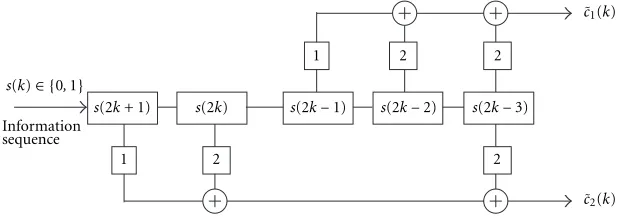
s(2k+ 1) s(2k) s(2k−1) s(2k−2) s(2k−3) s(k)∈ {0,1}
Information sequence
1 2 2
1 2 2
˜ c1(k)
˜ c2(k)
Figure3: 8-state space-time coding system model.
5. SIMULATIONS
In this section, we illustrate some simulation results to eval-uate the effectiveness and applicability of the proposed ML approaches. We consider the generator matrix form repre-sentation of the space-time coding system [15]. In this rep-resentation the stream of coded complexMPSK symbols are obtained by applying the mapping functionᏹto the follow-ing matrix multiplication:
c(k)=ᏹu(k)·G(modM), (39) whereu(k)=[s(lk+t−1), . . . , s(lk−t)]TandGis the genera-tor matrix withncolumns andl+srows andᏹis a mapping function that maps integer values ˜cito the codedMPSK sym-bols,ᏹ(˜ci)=exp(2π j˜ci/M).
The performance of the proposed methods was evalu-ated as a function of SNR (signal-to-noise ratio) based on the Monte Carlo simulations. Both conditional and uncon-ditional ML methods were tested for 200 Monte Carlo trials per SNR point across range of SNRs. In each trial, the estima-tion error of each parameter estimate from condiestima-tional and unconditional ML for the channel parameters were recorded. We consider the following two different cases.
Case1. 4PSK space-time code example shown in Figure 2 is considered withn=2,t=2 and the generator matrix
G=
2 0 1 0 0 2 0 1
. (40)
In this case, the coded 4PSK symbols obtained from two cur-rent information bits are transmitted over the first antenna, whereas the coded 4PSK symbols obtained from two pre-ceding bits are transmitted over the second antenna simul-taneously. The coded symbols are then transmitted through quasi-static fading channel matrix.
In Figure 4, we have plotted the estimation error ob-tained from conditional and unconditional ML for the chan-nel parameters as well as the corresponding CRBs. The esti-mation error experienced by the proposed estiesti-mation proce-dures at each iteration (SNR=10 dB) is shown in Figure 6.
Case2. A slightly more complicated space-time encoder with n=2,t=3 and the generator matrix
G=
2 0 1 0 0 2 0 1 2 2
(41)
is considered in this case. This example would be an 8-state code as shown in Figure 3.
In Case 2, the coded 4PSK symbols generated from [s(2k + 1), s(2k), s(2k −3)] are transmitted over the first antenna, whereas the coded 4PSK symbols obtained from [s(2k−1), s(2k−2), s(2k−3)] are transmitted over the second antenna simultaneously. The coded symbols are then trans-mitted through the quasi-static fading channel matrix.
5 10
SNR in dB
15 20
10−5 10−4 10−3 10−2 10−1 100
Channel
p
ar
amet
er
estimation
er
ro
r
n
or
m
Performance analysis: Case 1 Conditional ML Unconditional ML Conditional CRB Unconditional CRB
Figure4: Case 1: Channel matrix estimation error norm.
5 10
SNR in dB
15 20
10−5 10−4 10−3 10−2 10−1 100
Channel
p
ar
amet
er
estimation
er
ro
r
n
or
m
Performance analysis: Case 2 Conditional ML Unconditional ML Conditional CRB Unconditional CRB
Figure5: Case 2: Channel matrix estimation error norm.
both the conditional and unconditional ML together with their corresponding CRB’s for a range of SNR’s. Figure 7 shows the estimation error experienced by the proposed es-timation procedures at each iteration (SNR=10 dB).
Based on the simulations we made the following obser-vations:
(i) the proposed conditional and unconditional ML ap-proaches perform almost identically for high SNR val-ues. Moreover, conditional ML achieve conditional CRB for high SNRs;
(ii) since the unconditional cost function is dominated by only one term for high SNR, it results in exactly the same cost function as one would obtain for con-ditional ML estimation of θ. It is therefore expected that both conditional and unconditional cost func-tions yield similar estimates ofθat high SNR. Thus the unconditional ML approach also achieves conditional CRB for high SNR;
1 2 3 4 5 6 7 8 9 10
Iteration number 10−4
10−3 10−2 10−1 100
Channel
estimation
er
ror
nor
m
Convergence of the proposed algorithms: Case 1 Conditional ML Unconditional ML
SNR=10 dB
Figure6: Case 1: Convergence of the channel matrix.
1 2 3 4 5 6 7 8 9 10
Iteration number 10−4
10−3 10−2 10−1 100
Channel
estimation
er
ror
nor
m
Convergence of the proposed algorithms: Case 2 Conditional ML Unconditional ML
SNR=10 dB
Figure7: Case 2: Convergence of the channel matrix.
(iii) the unconditional approach requires more iterations than the conditional approach to converge, however, unconditional approach is more successful in reduc-ing channel estimation error norm at convergence for moderate SNR values.
6. CONCLUSIONS
CRB for high SNR values. Since the unconditional CRB pro-vides a looser bound, it is not as tight as exact CRB.
ACKNOWLEDGMENTS
This work was supported in part by the Research Fund of The University of Istanbul, Project numbers: B-924/12042001,
¨
O-1032/07062001, 1072/031297 and The Scientific and Technical Council of Turkey (TUBITAK) Project number 100EE006.
REFERENCES
[1] T. S. Rappaport,Wireless Communications Principles and Prac-tice, Prentice Hall, Upper Saddle River, NJ, USA, 1996. [2] V. Tarokh, N. Seshadri, and A. R. Calderbank, “Space-time
codes for high data rate wireless comunication: performance criterion and code construction,”IEEE Transactions on Infor-mation Theory, vol. 44, no. 2, pp. 744–765, 1998.
[3] A. F. Naguib, V. Tarokh, N. Seshadri, and A. R. Calderbank, “A space-time coding modem for high data rate wireless comu-nications,”IEEE Journal on Selected Areas in Communications, vol. 16, no. 8, pp. 1459–1478, 1998.
[4] Y. Li, G. N. Georghiades, and G. Huang, “EM-based sequence estimation for space-time codes systems,” inISIT ’2000, p. 315, Sorrento, Italy, June 2000.
[5] A. F. Naguib and N. Seshadri, “MLSE and equalization of space-time coded signals,” inVTC2000, pp. 1688–1693, Tokyo, Japan, Spring 2000.
[6] Z. Liu, X. Ma, and G. B. Giannakis, “Space-time coding and Kalman filtering for diversity transmissions through time-selective fading channels,” inProc. MILCOM Conf., vol. 1, pp. 382–386, Los Angeles, Calif, USA, October 2000. [7] C. Cozzo and B. L. Hughes, “Joint channel estimation and
data symbol detection in space-time communications,” in IEEE International Conference on Communications, vol. 1, pp. 287–291, 2000.
[8] S. Talwar, M. Viberg, and A. Paulraj, “Blind estimation of multiple co-channel digital signals using an antenna array,” IEEE Signal Processing Letters, vol. 1, no. 2, pp. 29–31, 1994. [9] L. E. Baum, T. Petrie, G. Soules, and N. Weiss, “A
maximiza-tion technique occurring in the statistical analysis of proba-bilistic functions of Markov chains,” The Annals of Mathe-matical Statistics, vol. 41, no. 1, pp. 164–171, 1970.
[10] G. K. Kaleh and R. Valet, “Joint parameter estimation and symbol detection for linear and nonlinear unknown chan-nels,” IEEE Trans. Communications, vol. 42, no. 7, pp. 2406– 2413, 1994.
[11] M. Erkurt and J. G. Proakis, “Joint data detection and channel estimation for rapidly fading channels,” inIEEE Globecom ’1992, pp. 910–914, Orlando, Fla, USA, December 1992. [12] P. Stoica and A. Nehorai, “MUSIC, maximum likelihood, and
Cramer-Rao bound,”IEEE Trans. Acoustics, Speech, and Signal Processing, vol. 37, no. 5, pp. 720–741, 1989.
[13] A. N. D’Andrea, U. Mengali, and R. Reggiannini, “The mod-ified Cramer-Rao bound and its application to synchroniza-tion problems,” IEEE Trans. Communications, vol. 42, no. 2/3/4, pp. 1391–1399, 1994.
[14] S. Haykin, Adaptive Filter Theory, Prentice-Hall, Englewood Cliffs, NJ, USA, 1996.
[15] S. B¨aro, G. Bauch, and A. Hansmann, “Improved codes for space-time trellis coded modulation,” IEEE Communications Letters, vol. 4, no. 1, pp. 20–22, 2000.
Hakan A. C¸ırpanreceived his B.S. degree in 1989 from Uludag University, Bursa, Turkey, the M.S. degree in 1992 from the University of Istanbul, Istanbul, Turkey, and the Ph.D. degree in 1997 from the Stevens Institute of Technology, Hoboken, NJ, USA, all in electrical engineering. From 1995– 1997, he was a Research Assistant with the Stevens Institute of Technology, working on signal processing for wireless
communica-tions. In 1997, he joined the faculty of the Department of Electrical-Electronics Engineering at The University of Istanbul. His cur-rent research activities are focused on signal processing and com-munication concepts with specific attention to channel estimation and equalization algorithms for space-time coding and multicar-rier (OFDM) systems. Dr. C¸ırpan received the Peskin Award from Stevens Institute of Technology as well as Prof. Nazim Terzioglu award from the Research fund of The University of Istanbul. He is a Member of IEEE and Member of Sigma Xi.
Erdal Panayırcıreceived the Diploma En-gineering degree in electrical enEn-gineering from Istanbul Technical University, Istan-bul, Turkey in 1964 and the Ph.D. degree in electrical engineering and system sci-ence from Michigan State University, East Lansing, Michigan, USA, in 1970. Between 1970–2000 he has been with the Faculty of Electrical and Electronics Engineering at the Istanbul Technical University, where he
was a Professor and Head of the Telecommunications Chair. Cur-rently, he is a Professor and Head of the Electronics Engineer-ing Department at IS¸IK University, Istanbul, Turkey. He is en-gaged in research and teaching in digital communications and wire-less systems, equalization and channel estimation in multicarrier (OFDM) communication systems, and efficient modulation and coding techniques (TCM and turbo coding). He spent two years (1979–1981) with the Department of Computer Science, Michigan State University, as a Fulbright-Hays Fellow and a NATO Senior Sci-entist. From August 1990 to December 1991 he was with the Center for Communications and Signal Processing, New Jersey Institute of Technology, as a Visiting Professor, and took part in the research project on Interference Cancelation by Array Processing. Between 1998–2000, he was Visiting Professor at the Department of Electri-cal Engineering, Texas A&M University and took part in research on developing efficient synchronization algorithms for OFDM sys-tems. Between 1995–1999, Prof. Panayırcı was an Editor for IEEE Transactions on Communications in the fields of Synchronizations and Equalizations.