S
CARED TOD
EATH?
I
NFORMATIONA
VOIDANCE ANDD
IAGNOSTICT
ESTINGYi Zhong
A dissertation submitted to the faculty of the University of North Carolina at Chapel Hill in par-tial fulfillment of the requirements for the degree of Doctor of Philosophy in the Department of
Economics.
Chapel Hill 2019
Approved by:
Donna Gilleskie
Luca Flabbi
Fei Li
Helen Tauchen
c
2019
Yi Zhong
ABSTRACT
YI ZHONG: Scared to Death?
Information Avoidance and Diagnostic Testing. (Under the direction of Donna Gilleskie)
To my loving parents, Chengyong Zhong and Qiaozhen Wang, who have unconditionally put all your love, time, and belief on me; who always support my pursuits and decisions; and who always
encourage me to follow my dreams.
ACKNOWLEDGMENTS
First, I would like to express my deepest appreciation to my advisor, Donna Gilleskie, without whose guidance and support this dissertation would not have been possible. I am greatly in-debted to Donna for her countless hours of help and profound belief in my work and my abilities. Throughout the process, Donna has taught me not only techniques to conduct rigorous economic researches, but also how to be a knowledgeable, enthusiastic, and careful researcher. Beyond aca-demics, Donna also sets a role model of a supportive and patient colleague, mentor, and friend for me. Her positive impact will always inspire me to keep improving and never forget why I started the process.
I would like to extend my deepest gratitude to my committee members, Fei Li, Luca Flabbi, Helen Tauchen, and Sally Stearns, for all their invaluable help with and guidance for my research. Their constructive comments and suggestions significantly improve the dissertation.
I am also very grateful to David Guilkey, who generously shares his program codes with me and patiently help me with my estimation programs.
I would like to acknowledge the help from Mathematica Policy Research, who provides me resources to improve my work. Specifically, I would like to thank David Mann and many other researchers there for their valuable and practical policy suggestions for my dissertation work.
TABLE OF CONTENTS
LIST OF TABLES . . . ix
LIST OF FIGURES . . . xi
1 Introduction . . . 1
2 Related Literature . . . 7
2.1 Is Preventive care beneficial? . . . 7
2.2 Demand for preventive testing . . . 8
2.3 Some people are information avoidant . . . 11
2.4 Belief-dependent utility and anticipatory utility . . . 13
3 Theoretical and Empirical Motivation . . . 17
3.1 Benchmark model . . . 17
3.2 Empirical evidence of relationship between pessimism and health anxiety . . . 23
3.3 Model with anticipatory utility . . . 25
4 Data . . . 30
4.1 Description of sample . . . 32
4.2 Key information . . . 32
4.3 Lifestyle behaviors . . . 34
4.4 Perception of health . . . 35
4.4.1 Calculation of subjective survival probability . . . 35
4.5 Employment . . . 38
5 Empirical Framework . . . 41
5.1 Individual decisionmaking process . . . 41
5.2 Estimable equations . . . 43
5.2.1 Demand equations . . . 44
5.2.2 Medical care behaviors . . . 47
5.2.3 Health production functions . . . 49
5.2.4 Health expectation processes . . . 52
5.3 Estimation strategy . . . 54
5.3.1 Attrition from the survey . . . 54
5.3.2 Initial conditions . . . 55
5.3.3 Distribution of unobserved heterogeneity . . . 55
5.3.4 Identification . . . 56
5.3.5 Likelihood function . . . 59
6 Estimation Results . . . 61
6.1 Data fit . . . 61
6.2 Estimation results . . . 63
6.2.1 Determinants of doctor visits . . . 63
6.2.2 Main contributors of blood sugar test . . . 66
6.2.3 Lifestyle behaviors . . . 69
6.2.4 Health production . . . 70
7 Policy Simulations . . . 75
7.1 Policy 1: Better information campaign or “nudge” to reduce health anxiety . . . 75
7.2 Policy 2: A mandatory screening program at age 60 . . . 78
7.3 Policy 3: A diabetes prevention program targeting at high-risk population . . . 80
8 Conclusion . . . 84
A Proofs in Theoretical Model . . . 87
B Alternative Models to Explain Information Avoidance . . . 89
B.1 Theory 1: Information averse . . . 89
B.2 Theory 2: Optimal belief . . . 91
B.3 Summary of other theories that explain information avoidance . . . 95
C Personality Measures in HRS . . . 98
D Specification of Quasi-structural Equations Estimated in the Model . . . 100
E FIML/DFRE Estimation Results . . . 102
F Data Fit Plots . . . 125
LIST OF TABLES
3.1 Regression analysis for pessimism and health anxiety . . . 25
4.1 Distribution of research sample by year and wave . . . 32
4.2 Summary statistics for endogenous variables . . . 33
4.3 Summary statistics for personality and exogenous variables . . . 40
5.1 Summary statistics of exclusion restriction variables . . . 57
6.1 Summary statistics of data fit . . . 62
6.2 Simulations: Impacts of reductions in barriers on doctor visits . . . 65
6.3 Simulations: Impacts of reductions in barriers on the probability of no blood sugar test (if undiagnosed) . . . 68
6.4 Simulations: Impacts of health information on lifestyle behaviors . . . 70
6.5 Simulations: Impacts of key determinants on blood sugar evolution . . . 72
6.6 Simulations: Impacts of key determinants on body mass production . . . 74
7.1 Policy simulation: A health anxiety improvement program . . . 77
7.2 Policy simulation: A national screening program at age 60 . . . 79
7.3 Policy simulation: A diabetes prevention program . . . 81
7.4 Policy simulation: A wellness program to improve exercise level . . . 83
D.1 Specification of Quasi-structural Equations Estimated in the Model . . . 101
E.1 Level of doctor visits (relative to a low level of visits) . . . 102
E.2 (Cont.) Level of doctor visits (relative to a low level of visits) . . . 103
E.3 Employment (relative to non-employment) . . . 104
E.4 (Cont.) Employment (relative to non-employment) . . . 105
E.5 Leve of exercise (relative to a moderate level of exercise) . . . 106
E.6 (Cont.) Level of exercise (relative to a moderate level of exercise) . . . 107
E.8 (cont.) Smoking and binge drinking . . . 109
E.9 No blood sugar test . . . 110
E.10 (cont.) No blood sugar test . . . 111
E.11 Nights in hospitals . . . 112
E.12 (Cont.) Nights in hospitals . . . 113
E.13 Blood sugar level evolution . . . 114
E.14 (Cont.) Blood sugar level evolution . . . 115
E.15 Body mass (BMI) production . . . 116
E.16 (Cont.) Body mass (BMI) production . . . 117
E.17 Self-report health status (relative to reporting a good health) . . . 118
E.18 Subjective 2-year survival probability . . . 119
E.19 Death . . . 120
E.20 Attrition from the survey . . . 120
E.21 Initial diabetes states (relative to taking a test and finding no diabetes) . . . 121
E.22 Initial self-report health status (relative to reporting a good health) . . . 122
E.23 Initial employment (relative to non-employment) . . . 123
E.24 Initial A1c . . . 123
LIST OF FIGURES
3.1 Value of (not) testing . . . 19
3.2 Marginal benefit and marginal cost of testing . . . 20
3.3 Simulated testing rate the benchmark model (Φ = 0.55,Ω = 0.45,M = 0.45and N=1,000,000) . . . 21
3.4 Blood sugar testing rate among undiagnosed individuals, by self-reported health status (HRS data) . . . 22
3.5 Blood sugar testing rate among undiagnosed individuals, by self-reported health status and pessimism level (HRS data) . . . 22
3.6 Timing of benchmark model with anticipatory utility . . . 26
5.1 Timing of decisionmaking . . . 42
A.1 Optimal lifestyle choice . . . 87
F.1 Data fit plots of number of doctor visits and employment by age . . . 125
F.2 Data fit plots of lifestyle behaviors by age . . . 126
F.3 Data fit plots of medical care behaviors and health outcomes by age . . . 127
F.4 Data fit plots of diabetes states by age . . . 128
CHAPTER 1
INTRODUCTION
According to the Centers for Disease Control and Prevention (CDC), consumption of preven-tive medical care is well below recommended levels. In fact, greater utilization of prevenpreven-tive care, especially for chronic conditions, has become a national health policy objective (e.g., the Healthy People 2020 Leading Health Indicators). Basic economic theory suggests that a reduction in the price of preventive care will increase the amount demanded. Recent U.S. reforms embodied in the Affordable Care Act (ACA) reflect this insight by requiring that insurance companies impose no consumer cost-sharing on approved preventive services. However, economic studies that exploit the exogenous changes in cost-sharing brought about by the RAND Health Insurance Experiment and the ACA reforms suggest that something else, other than price, may have an important im-pact on demand for preventive services. For example, data from the RAND Health Insurance Experiment suggest that, even with zero out-of-pocket costs, the majority of adult males used no preventive care at all for three years (Newhouse and Group, 1993). Using more recent data, some researchers find that reductions in the price of screening (for high cholesterol, breast cancer, dia-betes, etc.) encourage its use (Finkelstein et al., 2012), while others find that consumers are not very sensitive to the price of preventive care (Sabik and Bradley, 2016; Simon et al., 2016; Xu et al., 2016; and Cabral and Cullen, 2017).
utility, which suggests that individuals acquire utility directly from expectations, or anticipations, about the future. That is, the model should consider health anxiety, which represents the stress or disutility associated with the anticipation of positive (i.e., bad outcome) test results, as an additional cost in an individual’s forward-looking, dynamic decision making process (Caplin and Leahy, 2001; K˝oszegi, 2003; and Caplin and Eliaz, 2003).
Although widely discussed in the economic theory literature, this concept of health anxiety re-mains underexplored empirically because its measurement is, to date, elusive. That is, there is no validated survey measure of individual avoidance of particular preventive care screenings/testings due to anxiety about the results. Alternatively, and as I propose, this kind of behavior can be identified or picked up using variation in particular personality characteristics after modeling the many other potential explanations for non-participation in a recommended testing. In this paper, health anxiety is defined as the independent effect of pessimism on an individual’s screening be-havior while conditioning on other endogenous explanations. This definition follows the economic theoretical literature as people who are more pessimistic are more likely to anticipate a bad result and thus suffer from the anticipatory disutility. Additionally, this definition is also supported by empirical evidence showing that pessimism is directly correlated with an individual’s response for why she would avoid a screening test as “fear of the possibility of receiving a positive test result”, after conditioning on key individual characteristics and other personality measures.1
Therefore, this study evaluates the roles of many contributors, including health anxiety, to type-2 diabetes screening behavior by developing a dynamic, stochastic model of an individual’s decisions about doctor visits (at which a blood sugar test may or may not be administered), other health-related behaviors, and employment where underlying disease state governs diabetes stage, individuals have imperfect information about their true health (if untested), and health anxiety is identified by an individual’s pessimism level.2 By incorporating health anxiety, this study provides a richer framework for understanding an individual’s non-participation in diabetes screening.
Type-2 diabetes, or diabetes mellitus type 2, is a long-term metabolic disease characterized by a high blood sugar level over a prolonged period because the cells fail to use insulin properly to process glucose.3 Type-2 diabetes is primarily caused by obesity and lack of exercise and com-monly manifests in adulthood. The common treatments include exercise, diet adjustment, oral medication, and insulin shots. Poorly-managed diabetes can progress irreversibly to severe stages and cause other complications such as blindness, lower extremity amputation, heart attack, and stroke (Oster, 2018a; Mroz et al., 2016; and World Health Organization, 2003). Type-2 diabetes provides a good setting to study demand for health information and health anxiety for three rea-sons. First, the asymptomatic features of diabetes enable me to examine screening behavior and health anxiety without worrying about the confounding effects of disease symptoms on medical care consumption behavior. Second, because diabetes screening is the least invasive compared to other types of preventive tests such as a mammogram, prostate, or cancer screening, it helps to minimize the disutility associated with the testing procedure itself when examining the disutility from health anxiety. Third, diabetes is not curable once diagnosed, but treatments are available to control its progression and the symptoms. This attribute makes diabetes screening both scary and useful, creating an interesting tradeoff problem for the patients.
In addition, understanding the diabetes screening behavior is of significant policy importance. Diabetes is a prevalent and growing chronic condition. There are 29 million Americans (i.e., 1 out of every 11 Americans) living with diabetes, 86 million (i.e., 1 out of every 3 Americans) living with pre-diabetes and 1.7 million new cases diagnosed each year.4 Because diabetes is
asymptomatic in early stages, preventive screening is important for early diagnosis. According to the CDC, up to 25 percent of U.S. adults who have diabetes do not know that they have it, and 90 percent of people with prediabetes are unaware. Without any lifestyle changes, 15 to 30 percent of people with prediabetes will develop type-2 diabetes within five years (CDC Division of
3With type-1 diabetes, a high blood sugar level results from the failure of the pancreas to produce any insulin. The
cause of type-1 diabetes is not clear and it usually starts in childhood. Type-1 diabetic patients have to take a routine insulin shot as a replacement of pancreatic function. In this paper, ‘diabetes’ refers to type-2 diabetes.
4Pre-diabetes is the precursor stage of type-2 diabetes, when the blood sugar level is higher than normal but not
Diabetes Translation, 2014). Diabetes is more costly to treat and leads to worse health outcomes if detected later (Mroz et al., 2016). The annual costs of diabetes account for 20 percent of national medical care costs ($176 billion in direct medical costs and an additional $69 billion associated with reduced productivity in 2012). Importantly, less than half of individuals for whom diabetes screening is recommended comply (Kiefer et al., 2015). An improvement in diabetes screening behavior could have both individual and societal impacts (American Diabetes Association, 2013). The various contributors to an individual’s diabetes screening behavior are explicitly delineated in the theoretical model. The contributors are: health anxiety, monetary and time costs of doctor visits and tests; the marginal effectiveness of different types of medical and non-medical inputs for controlling blood sugar levels; an incorrect perception of health; and life expectancy. To reflect the fact that physicians may also play an important role in an individual’s screening behavior, I assume that an undiagnosed individual, with at least one doctor visit during a two-year period, may receive a diabetes screening with some probability. Prior to learning her true disease state (which can only be verified with a blood sugar test), an individual bases her decisions about medical care use and other health behaviors on her prior known disease state and perceived, or subjective, health status. The subjective and true disease states reflect the degree to which information about one’s own health is imperfect. Subjective beliefs about one’s health are captured by self-reported health status and a subjective survival probability.
My primary data source is the Health and Retirement Study (HRS) survey and its linked biomarker data. The HRS survey data are longitudinal, with biennial observations from 1992 to 2014. New cohorts enter the survey every six years. I use data from 2004 to 2012 due to the availability of blood sugar test information. The survey provides information about an individual’s employment, health-related behaviors, medical care consumption, diabetes status, and blood sugar testing behavior. The linked biomarker data collect and test respondents’ blood samples biennially from 2006 to 2012, from which I can observe an individual’s true disease state.
CHAPTER 2
RELATED LITERATURE
2.1 Is Preventive care beneficial?
In general, this paper is related to a vast amount of literature about preventive care. In semi-nal work by Ehrlich and Becker (1972), preventive care is introduced to the medical care demand discussion (among economists) as “self-protection” and “self-insurance”. Self-protection encom-passes primary preventive care (e.g., flu vaccine) as it can reduce the probabilities of bad health states; while self-insurance captures secondary primary care (e.g., diabetes and cancer screening) as it reduces the size of the loss in the bad states if detected early. Their theoretical model sug-gests that, because market insurance and self-insurance are substitutes, a moral hazard problem may arise if the price of market insurance is not negatively related to the amount spent on protec-tion. However, Ehrlich and Becker (1972) assume that preventive care is always beneficial. Taking this assumption as given, following studies proceed to discuss the optimal coverage for preventive care. Howard (2005) claims that there is always an age beyond which the costs of early detection outweigh the benefits.1 Herring (2010) claims that the enrollee turnover among health insurers explains the suboptimal provision of coverage of preventive health care: the financial benefits of preventive care accrue in the future and some of the benefits to an insurer will be lost when the en-rollees change health plans. Ellis and Manning (2007) provide more theoretical support claiming that it is always desirable to offer at least some insurance coverage for preventive care.
More recent studies revisit the assumption about the benefits of preventive care and provide mixed empirical evidence. Mroz et al. (2016) find that screening tests and early diagnoses of type-2 diabetes are beneficial. They estimate a dynamic multistage duration model and find that earlier
1However, his model assumes that individuals are risk neutral and that screening occurs every period, and it
diagnosis of diabetes delays the onset of lower extremity complications (LECs) and amputation. For example, a one-year delay in the diagnosis of diabetes increases the probability of LECs five years later by 11 percent and the probability of transition to high severity LECs by 27 percent. Kim et al. (2017) use the design that disease risk classification are discontinuous based on the biomarker readings (e.g., fasting blood sugar, BMI, and cholesterol) to examine whether people respond to disease risk information provided by the National Health Screening Program in Ko-rea. They find evidence of increased diabetes medication use and weight loss around the high-risk threshold of diabetes only, while little or no difference in behaviors and health outcomes around the medium-risk threshold for diabetes and thresholds for obesity and hyperlipidemia. One lim-itation of the study is that they do not control for how much health information individuals have before the national screening program. Additionally, advice and treatment provided by physicians may depend on the biomarker reading proximity to the thresholds, making the discountinuity de-sign vulnerable. Iizuka et al. (2017) also use the regression discontinuity dede-sign of biomarker risk classification to examine the effect of mandatory checkup in Japan. They find that people respond to heath information by having more doctor visits, but their health or predicted risk of mortality and serious complication does not improve. Gandjour (2009) claims that prevention in the gen-eral population leads to expenditures for additional diseases that are larger than the savings from postponing an expensive last year of life. However, he does not consider the gained value of life of people live longer. Preventive testing may also have negative externalities. For example, Oster et al. (2010) identify adverse selection in the long-term care insurance market due to the increased private information associated with genetic testing. Filipova-Neumanna and Hoy (2014) construct a theoretical model to analyze the moral hazard that potentially results from the increased amount of information provided by screening and genetic tests.
2.2 Demand for preventive testing
age but increases with health insurance coverage and schooling. Finkelstein et al. (2012) explore the exogenous cost shock of the Oregon Medicaid lottery and find that insurance is associated with a significant and large increase in compliance with recommended preventive care: a 20 (15) percent increase in the probability of ever having blood cholesterol (sugar) checked and a 60 (45) percent increase in the probability of having a mammogram (pap test) within a year. Sabik and Bradley (2016) employ a quasi-experiment framework to analyze the effect of the expansion to near-universal health insurance coverage in Massachusetts on breast and cervical cancer screening. They find a significant but mild increase (i.e., 4-7 percent) in the screening rates. Even with near-universal health insurance, the testing rates are not close to near-universal: 77.8 percent for mammogram and 75.1 percent for pap test annually. Using a cross-sectional national survey in Mexico, Pag´an et al. (2007) find that health insurance coverage improves preventive screening utilization for high cholesterol and diabetes among people ages 50 and older.
However, some other studies find that preventive care consumption is not very responsive to price and insurance coverage. The RAND Health Insurance Experiment revealed little price sen-sitivity of preventive care. Even with zero out-of-pocket costs, the majority of adult males used no preventive care at all for three years (Newhouse and Group, 1993). Simon et al. (2016) explore the 2014 Affordable Care Act (ACA) Medicaid expansions and find mixed effects on a variety of preventive care behaviors. There is an increased use of dental visits, mammogram, and cancer screening, but no detectable change for flu shots, HIV tests, or pap tests. Cabral and Cullen (2017) use a health insurance design that increases the price of non-preventive care while decreasing the price of preventive care and they find that preventive care utilization does not increase, and even declines, due to the differential price change. Xu et al. (2016) use the Medical Expenditure Panel Survey (MEPS) and variation in timing of state mandates for coverage of colorectal, cervical, and prostate cancer screening; they find that state mandatory coverages do not increase cancer screen-ing rates.
(2013) examines the impact of three factors on breast cancer screening behavior of women aged 50-64 in the UK: the disutility of screening, the effect of screening on survival probability, and the discount factor. The results suggest the greatest driver to be forward-looking behavior, although education differences in mammography attendance are mainly due to lower disutilty of screening among higher educated women rather than different time preferences. Montoy et al. (2016) analyze data from a randomized clinical trial that assigned patients aged 13-64 to opt-in, opt-out, and active choice arms of HIV test offers. The opt-out arm has the highest acceptance rate (65.9%), then active choice arm (51.3%), and lastly the opt-in arm (38%). The determinants of demand for preventive care are also heterogeneous for different tests and groups of people. Bouckaert and Schokkaert (2016) show that influential factors for different preventive procedures are different. Specifically, poor individual health decreases breast cancer screening and dental prevention and increases vaccination, cholesterol screening, blood pressure, and blood sugar screening. They also find a positive income effect for dental prevention and find higher mortality risk to improve take-up of breast cancer screening. Nuscheler and Roeder (2015) find that the most important determinants of preventive care consumption differs between men and women: time preference and risk aversion significantly impact mens immunization decisions while health information impacts the immunization decisions of both men and women.
2.3 Some people are information avoidant
Women with family history, who seem to benefit more and know more information about the dis-ease, are more likely to delay. Among reasons for delay, 25 percent of the subjects choose fear. Lerman et al. (1996) present that 40 percent of high-risk patients who are offered a test for ge-netic susceptibility to breast and ovarian cancer declined the test. A similar study by Lerman et al. (2004) on a type of colon cancer discovers that 57 percent of high-risk individuals declined to test. Thompson et al. (2002) find those who declined to participate in a genetic test and counseling for breast cancer report greater anticipation of negative emotional responses to testing. Persoskie et al. (2014) find that cancer worry, but not the perceived risk of cancer, predicted doctor avoidance in respondents aged 50 and older. Consedine et al. (2004) review studies and recognize that “a fear of finding something wrong” and “it’s better not to know” are key barriers of breast cancer screening. Cutler and Hodgson (2003) find even among a sample with a parental history of Alzheimer’s disease, 32 percent of subjects declined to take a genetic test for Alzheimer’s. Lyter et al. (1987) use the Pittsburgh cohort of the Multicenter AIDS Cohort Study and show that only 61 percent of the gay and bisexual males, who are at high risk of AIDS, accepted the invitation to learn the results of their HIV infection test. Half of the non-participants choose the reason “they would be too worried about developing AIDS if the test is positive” and about a third of them choose “they would be unable to cope with a positive result”. Sullivan et al. (2004) also demonstrate that failure to return for HIV test results is very common among people at high risk for HIV infection and the failure rate is even higher among people with higher perceived risks of HIV infection. Additionally, they report that 25 percent of respondents cite fear of getting test results as an important barrier. Hightow et al. (2003) observe 55 percent of study subjects failed to return for their HIV testing results and the failure rate among those who actually tested positive is even higher. Thornton (2008) conducts a field experiment in rural Malawi and finds that only 34 percent of the participants without a monetary incentive learned their HIV test results.
tested. Stunningly, results show that 15 percent of students are willing to pay to avoid the test and the top reason is that “it will cause me unnecessary stress or anxiety if I test positive”. Oster et al. (2013) explore the decision to undergo genetic testing for Huntington Disease. In their sample, fewer than 10 percent of individuals at risk for the disease actually pursue predictive testing during the 10-year study period. Wu (2003), using the HRS and MEPS data, finds that self-reported health status is positively and significantly associated with having a flu shot, but negatively associated with having a pap smear, breast exam, mammogram and prostate check. The negative correlation between health status and screening tests may be due to fear or anxiety associated with learning health information because those who are more pessimistic are less likely to do those tests.
2.4 Belief-dependent utility and anticipatory utility
This study is also closely related to a growing amount of theoretical literature that incorporates behavioral and psychological factors using belief-dependent utility. It is common in modern eco-nomics to assume that humans have unlimited cognitive ability to make optimal decisions. Thus, the value of information exactly equals the extent to which it improves decisionmaking and it cannot be negative (B´enabou and Tirole, 2016). However, often times, human decisionmaking involves a combination of emotions and limited cognitive ability. As Schelling (1988) describes, the mind is a consuming organ. Information may have both instrumental and direct value through belief-dependent utility and, therefore, lead to information avoidance. B´enabou and Tirole (2016), Gino et al. (2016), and Epley and Gilovich (2016) provide good summaries and explanations about motivated belief and reasoning. They emphasize that beliefs often contain important psychological value. Thus, people tend to manipulate their collection and processing of information in ways that depart from strict Bayesian inference, trading off the affective value of belief distortion against the costly mistakes they may induce.2
The motivation for motivated belief is twofold. First, belief has instrumental value; for exam-ple, an individual prefers to hold a distorted belief to solve a self-control problem. Second, belief
can have direct utility through anticipatory utility, which means agents’ experience feelings of an-ticipation prior to the resolution of uncertainty into utility (Caplin and Leahy, 2001). Motivated belief can be formed by motivated collection (e.g., attorneys collect evidence to support their own side), motivated avoidance (e.g., heath anxiety prevents people from taking tests), reality denial, and self-signaling. Golman et al. (2016) provide a summary of explanations for information avoid-ance. They categorize the reasons into two types: hedonically-driven information avoidance, which includes reasons such as anxiety, optimism maintenance, and belief investment; and strategically-driven information avoidance, which includes resisting temptation, motivation maintenance, save it for later, etc. Karlsson et al. (2009) use the fact that investors are less likely to check their portfolios in down and flat markets than in up markets as empirical evidence of the ostrich effect, which indicates that individuals regulate the impact of good and bad news on their utility by how intently they attend to the news. Thunstr˝om et al. (2016) construct a model with strategical self-ignorance showing that guilt aversion and present-biased individuals will avoid information that suggests negative future impacts of current pleasurable activities. In a lab experiment, they find that 58 percent of participants choose to ignore free calorie information about their chosen meals, and those participants consume significantly more calories.
setting where individuals have time-inconsistent preference (or hyperbolic discounting time pref-erence) and the individuals are allowed to be naive about their time inconsistency. Empirically, they find that both present bias and naivety of the individuals explain the high rate (i.e., 25 percent) of non-participation in mammography screening in the United States. But their study assumes that mammography lowers the probability of bad health or the death rate and skips the intermediate steps about patients behavioral changes. Hoy et al. (2014) use a model of ambiguity aversion to explain the low uptake rate of genetic testing for breast and ovarian cancer. When the individual takes a genetic test, she faces the uncertainty of receiving “good” or “bad” news that will improve or deteriorate her belief about the probability of having the disease. However, without taking the genetic test, she is free to stick to her prior belief (e.g., average probability of having breast cancer in the population). An ambiguity averse person may choose to avoid genetic testing in order to avoid this ex-ante lottery between a deterioration and an improvement in beliefs.
CHAPTER 3
THEORETICAL AND EMPIRICAL MOTIVATION
Before presenting a detailed dynamic stochastic model, I use a three-period theoretical model to describe the demand for diagnostic testing in a simplified environment. I present two versions of the model in this section. The benchmark model uses the classical expected utility framework and shows that this framework can only explain the average screening test behavior. It is not enough to explain the heterogeneous screening behavior by individuals’ pessimism levels. Then, to support my definition of and approach to identify health anxiety in the empirical analysis, I provide em-pirical evidence from the University of North Carolina Alumni Heart Study (UNCAHS) showing that pessimism is directly and significantly associated with individuals’ health anxiety levels. This evidence supports the hypothesis that the heterogeneous screening behavior by individuals’ pes-simism levels can be explained using health anxiety. Lastly, following Caplin and Leahy (2001), I extend the benchmark model by adding an anticipatory utility component to capture an individ-ual’s anticipatory fear of receiving a positive test result if she decides to take a screening test. I use this model to characterize how pessimism enters an individual’s desicionmaking and explain how it serves to identify the effect of health anxiety.
3.1 Benchmark model
Model setup
Consider a three-period game. Att= 0, nature moves to decide an individual’s state of the world s∈ {0,1}, wheres= 1indicates that the individual has diabetes ands= 0indicates she does not. The decision maker then evaluates her payoffs and chooses her behaviors (actions). I describe the components of decisionmaking here.
(2) Actions:
– A binary screening test choice (b ∈ {0,1}) at t = 1. If a diabetes screening is performed (b = 1), the test result is revealed right beforet = 2and the individual knows her true state of the world. Furthermore, if she is diagnosed, she can receive treatmentM at periodt = 2; otherwise she does not know the state of the world and cannot receive any treatment.
– A binary lifestyle action (a∈ {0,1}) att= 2. The actiona= 1indicates a very healthy and careful lifestyle (e.g., more exercise, no smoking, no binge drinking, and sugar-less diets) anda= 0indicates normal or usual lifestyle.
(3) Payoffs: payoffu(s, a)is realized by the end oft= 2where
u(0,0) = 1 no diabetes, normal lifestyle
u(0,1) = 1−Φ no diabetes, very healthy lifestyle
u(1,0) =−Ω with diabetes, normal lifestyle
u(1,1) = 0 with diabetes, very healthy lifestyle
I normalize the utility from the matched lifestyle choice and the true state of world and assume
Φ, Ωand M all lie within [0,1]. That is, the utility of “no diabetes, normal lifestyle” and “with diabetes, very healthy lifestyle” are normalized to be 1 and0, respectively; and the utility from a mismatched lifestyle choice is lower than the matched one. Additionally, the utility payoff is always lower for those with diabetes in order to capture diabetes’ negative impact on utility through health. There is also a monetary (and time) cost,c, of taking a screening test.
Analysis
I solve the model backward. For period 2 behavior:
Lemma 3.1If the individual chooses not to test (b = 0), her optimal lifestyle choice (a∗) is:
a∗ =
0 ifπ < Φ
Ω+Φ
(The proof is shown in Appendix A.)
Leta∗be the optimal lifestyle givenπas shown in Lemma 3.1. Then, the expected value of not taking a test,Vb(π)whereb= 0, is:
V0(π) = πu(1, a∗) + (1−π)u(0, a∗)
=
1−π(1 + Ω) ifπ < Ω+ΦΦ
(1−π)(1−Φ) ifπ ≥ Φ Ω+Φ
(3.1)
If an individual takes a test and finds out that she has diabetes, she will choose a healthy lifestyle sinceu(1,1) > u(1,0); if she finds out that she does not have diabetes, she will choose a normal lifestyle given thatu(0,0)> u(0,1). Hence, the value of taking a screening test (b= 1) is:
V1(π) = π(u(1,1) +M) + (1−π)u(0,0) = 1−π(1−M)
(3.2)
The values of the testing alternatives are depicted in Figure 3.1.
Therefore, the marginal benefit from taking a screening test is:
M B = V1(π)−V0(π)
=
π(M + Ω) ifπ < Ω+ΦΦ
π(M −Φ) + Φ ifπ ≥ Φ Ω+Φ
(3.3)
The marginal cost of taking a screening test isM C =c. The individual decides to take a screening test or not according to the marginal benefit and marginal cost as shown in Figure 3.2.
Figure 3.2: Marginal benefit and marginal cost of testing
Using this framework and allowing the marginal cost to be random, I simulate the testing pattern. I assumeΦ = 0.55,Ω = 0.45, andM = 0.45.1 The value ofπis drawn from a normal distribution
with mean 0.5 and variance 0.3. Values smaller than 0 or larger than 1 are replaced with the boundary values (i.e., 0 and 1). The cost of taking a test is drawn from a normal distribution with mean 0 and variance 0.5.2 If M B −M C ≥ 0, the individual takes a screening test, otherwise she does not. The simulated testing pattern for N=1,000,000 individuals is shown in Figure 3.3. The testing rate increases withπat first and then remains constant. It is because, in the beginning, both information and expected treatment value increase, making people more likely to screen.
1According to the theoretical model and the simulation technique, different values ofΦandΩwill only change
the cutoff value ofπat which we observe the highest rate of testing.
2I do not restrict the cost to be positive in the current simulation. That is, an individual may get more value from
After a cutoff point, information value starts to decrease, while the expected utility from treatment continues to increase, making the screening rate almost constant withπ.3
Figure 3.3: Simulated testing rate the benchmark model (Φ = 0.55, Ω = 0.45, M = 0.45and N=1,000,000)
Implication
To examine whether my theoretical model explains individuals’ behaviors in reality, I compare the simulated testing behaviors to the one I observe in the Health and Retirement Study (HRS) data. Ideally, I want to plot the testing behavior along with the individual’s subjective belief of having diabetes. However, I do not observe this exact measure in the data. Instead, I use an individual’s self-reported health status as the measure of subjective belief of having diabetes (π). As we observe in Figure 3.4, the testing rate increases at lower values ofπand remains constant afterward. This shape is almost identical to the one I simulated based on the theoretical model, indicating that the theoretical model with information and treatment value characterize individuals’ average behavior well.
But, are the information and treatment values enough to explain the testing behavior? If we divide people in the HRS sample into two groups based on their pessimism levels, we observe that their testing rates are different conditional on self-reported health status (Figure 3.5). According
3For a scenario with only information value, the simulated screening pattern is concave along withπ. The concave
Figure 3.4: Blood sugar testing rate among undiagnosed individuals, by self-reported health status (HRS data)
Figure 3.5: Blood sugar testing rate among undiagnosed individuals, by self-reported health status and pessimism level (HRS data)
does not affect the information or treatment value of the test.4 This testing pattern indicates that
there is something missing in our model to explain the different testing behaviors among people with different personalities. Following the theoretical model, health anxiety could serve as a good explanation since pessimistic individuals, who are more inclined to anticipate a bad outcome in the future, are suffering greater health anxiety and, thus, are more likely to avoid testing. In the next subsection I provide empirical evidence to support the hypothesized relationship between pessimism and health anxiety and therefore to support the argument that the heterogeneous testing behavior by pessimism in fact reflect the effect of health anxiety.
3.2 Empirical evidence of relationship between pessimism and health anxiety
The HRS data contain much of the information necessary to conduct an empirical study of the contributors to diabetes screening behavior. However, this data set does not have a measure of health anxiety. Rather, I identify anticipatory utility by a measure of pessimism. In order to claim a direct relationship between pessimism and health anxiety, I use data from the University of North Carolina Alumni Heart Study (UNCAHS), which includes measures of pessimism and health anx-iety. UNCAHS is an on-going survey that follows about five thousand individuals enrolled as students at UNC during 1964-1966 who completed the Minnesota Multiphasic Personality Inven-tory while in school. The second wave of the survey was collected in 1986, almost 20 years after graduation, with the original purpose of assessing hostility as a risk factor for coronary heart dis-ease. Over time, the survey has collected information about health, personality, and socioeconomic wellbeing.
The UNCAHS collected personality information using the NEO personality inventory. This inventory assesses individuals’ personalities following the “big five” personal traits: neuroticism, extraversion, openness, agreeableness, and conscientiousness. Among the collected items under neuroticism, one item states “I often worry about things that might go wrong”, which (according to the literature) serves as a good measure of pessimism. Higher values (scored from 1 to 100) imply
4Even if we argue that pessimism actually complements my coarse measure of subjective probability of having
greater pessimism. I create an individual-level average value using responses from two separate waves. This item is almost identical to ones collected in the HRS, which I use as a pessimism measure (for example, one item in HRS pessimism measure is “If something can go wrong for me it will”; see the data chapter for more information). Additionally, UNCAHS provides a good measure for health anxiety. Among the reasons why a woman does not have a mammogram, one is “fear the possibility of finding breast cancer”.5 Responses range from “not at all” (1) to “enough
to prevent me” (4). This unique and direct measure of health anxiety, where a higher score implies the individual is more health anxious, allows me to empirically examine the relationship between pessimism and health anxiety.
Simple correlation
I use these two variables to assess the correlation between pessimism and health anxiety. In a sample of 1,606 individuals, I find a statistically significant and positive correlation of 0.134 with a P-value of 0.000.6 I also perform a robustness check using the pessimism response from each of
the two waves and find similar results.
Regression analysis
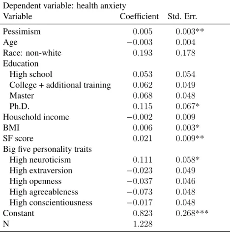
In order to determine whether the positive and statistically significant relationship between pes-simism and health anxiety is due to some confounding factors, I conduct a regression analysis including an individual’s “big five” personality traits. Additional included variables are age, race, education, income, body mass, and SF5 total score, which measures an individual’s current health, memory, ability to cope with stress, financial well-being, and support system. The results are shown in Table 3.1. The results indicate that pessimism is still positively and significantly corre-lated with health anxiety even after controlling for many other variables. This empirical evidence
5Other reasons include: (1) cost too expensive; (2) concerns about radiation exposure; (3) possibility the procedure
could be painful; (4) possibility of being embarrassed by procedure; (5) inconvenience of being too busy; (6) feel in good health and do not have symptoms; (7) not necessary if my doctor does not recommend.
6The large attrition happens when restricting the sample to individuals with non-missing health anxiety values. At
Table 3.1: Regression analysis for pessimism and health anxiety
Dependent variable: health anxiety
Variable Coefficient Std. Err.
Pessimism 0.005 0.003**
Age −0.003 0.004
Race: non-white 0.193 0.178
Education
High school 0.053 0.054
College + additional training 0.062 0.049
Master 0.068 0.048
Ph.D. 0.115 0.067*
Household income −0.002 0.009
BMI 0.006 0.003*
SF score 0.021 0.009**
Big five personality traits
High neuroticism 0.111 0.058*
High extraversion −0.023 0.049
High openness −0.037 0.046
High agreeableness −0.073 0.048
High conscientiousness −0.017 0.048
Constant 0.823 0.268***
N 1.228
** indicates significance at 5% level and * indicates 10% level.
provides support for my approach to identify and define health anxiety. In the next subsection, I outline a second theoretical model, which incorporates anticipatory utility (i.e., health anxiety in this case), to show how health anxiety enters an individual’s decisionmaking process and how pessimism relates to health anxiety.
3.3 Model with anticipatory utility
Model setup
Figure 3.6: Timing of benchmark model with anticipatory utility
0 1 2
Nature decidess∈ {0,1}
Subjective beliefπ
DM decides screeningb∈ {0,1}
Anticipatory utility ifb= 1
Test result revealed ifb = 1
DM decides actiona∈ {0,1}
(3) Payoffs:
– At period 1:
– If an individual decides to screen (b = 1), she receives the disutility from the antic-ipatory anxiety of a positive test result, −φ(π, γ), where π is the subjective belief of having diabetes and γ is the pessimism level of the individual. This anxiety term is discussed in more detail in the next section.
– If an individual decides not to screen, thenφ = 0as she does not need to suffer antici-patory anxiety about the test result.
– At period 2: payoffu2(s, a)is realized as below. Additionally, the individual receives
medi-cal treatmentM if she is screened and is diagnosed with diabetes.
u2(0,0) = 1 no diabetes, normal lifestyle
u2(0,1) = 1−Φ no diabetes, very healthy lifestyle
u2(1,0) =−Ω with diabetes, normal lifestyle
u2(1,1) = 0 with diabetes, very healthy lifestyle
Analysis
anticipatory utility term, the expected value in period 1,Vb(π, γ), becomes:
Vb(π, γ) =
0 + maxa[Eπu(s, a)] ifb= 0
−φ+Eπ[maxau(s, a)] +π∗M ifb= 1
=
0 +π×u2(1, a∗) + (1−π)×u2(0, a∗) ifb= 0
−φ+π×(u2(1,1) +M) + (1−π)×u2(0,0) ifb= 1
(3.4)
Therefore, the marginal benefit from taking a screening test is:
M B = V1(π, φ)−V0(π, φ)
= −φ
|{z}
health anxiety
+Eπ[max
a u(s, a)]−maxa [Eπu(s, a)]
| {z }
information value
+ π∗M | {z }
treatment value =
−φ+π(M + Ω) ifπ < Ω+ΦΦ
−φ+π(M −Φ) + Φ ifπ ≥ Φ Ω+Φ
(3.5)
For now, let’s assume the monetary cost of taking a test is normalized to zero. Then, in the individual’s optimization problem, the cost of taking a screening test is the health anxiety psy-chic cost, −φ. The benefit of taking a screening test comes from two parts: first, the individ-ual knows her disease state and could choose a lifestyle action contingent on the disease state (Eπ[maxau(s, a)]−maxa[Eπu(s, a)], information value); and second, the individual can receive medical treatment if she is diagnosed with diabetes (π∗M, treatment value). The individual takes a screening test if the health anxiety cost is smaller than the information and treatment value; otherwise, she chooses not to screen.
Health anxiety
show how pessimism can help us capture the anxiety associated with anticipating a bad test result indirectly.
First, let’s think about how an individual forms her anticipation of a positive test outcome. For each individual, there is an objective distribution of the probability of having diabetes (π0).
The individual does not observe the distribution, but she forms a subjective perception about the distribution (πs) based on signals or information about her true health (e.g., easily feeling tired, easily feeling hungry, or being able to run 5 miles in an hour) that she receives in her daily life. Ideally, an individual will do rational Bayesian updating to form her subjective perception every time she receives a signal about her health. However, it is very likely that the health perception is impacted by psychological reasons (B´enabou and Tirole, 2016; Epley and Gilovich, 2016; and Goodwin and Engstrom, 2002). Specifically, a pessimistic individual who “usually expects the worst in uncertain times”, would put higher weights on the bad signals of her health and form a biased perception of her probability of having the disease.7
I use the first and second moments to describe the subjective perception distribution. The subjective probability in the theoretical model,π, captures the mean of the subjective distribution (π =E[πs]). There is also a variance of this subjective distribution (V ar(πs) =E[(πs−E[πs])2]). πcaptures, on average, how likely the individual believes she has diabetes and the variance captures how certain the individual is about this average probability. A more pessimistic individual puts higher weights on the bad signals. As a result, her variance would be smaller whenπis high and would be larger whenπ is low. In other words, when the pessimistic individual believes that, on average, she is very likely to have diabetes, she will be more certain about the belief; while when she believes that, on average, she is healthy, she will be more uncertain about this belief since she “rarely counts on good things happening to her”. Therefore, the variance of the subjective
7A pessimistic individual is defined as someone more likely to believe (1) if something can go wrong for me, it
distribution is a function of pessimism,γ. Specifically,
V ar(πs) =E[(πs−E[πs])2] =σ0−(π− 1
2)∗γ (3.6)
I now explain how anticipatory anxiety is related to the subjective perception. Following Caplin and Leahy (2001), the anticipatory anxiety is assumed to be a function of the mean and variance of the uncertainty.8 Since the anxiety is associated with anticipating a bad outcome in the future, it is reasonable to assume that the anxiety is increasing in the mean probability of the perception (π). That is, the individual is more anxious when she anticipates that, on average, a bad outcome is very likely. The relationship between health anxiety and the variance of belief is not linear. When π is high, the anticipatory anxiety is decreasing in the variance of the belief: as the individual is more certain that she will receive bad news in future, she suffers larger anxiety associated with anticipating a bad news. When π is low, the anxiety is increasing in the variance of the belief, as the individual is more uncertain that she is healthy. A simple functional form that satisfies this assumption is in equation (3.7). We have equation (3.8) after substitutingV ar(πs)with its function in equation (3.6).
φ(π, V ar(πs)) =α0+α1π+α2( 1
2−π)V ar(πs) (3.7)
φ(π, γ) = (α0+ 1
2α1σ0) + (α1−α1σ0)π+α1(π− 1 2)
2γ (3.8)
With some assumptions on the parameter values, the anticipatory anxiety is increasing in both
π andγ. However, because the subjective average probability, π, also affects the expected
infor-mation and treatment value of taking a screening test, I cannot disentangle those three parts to identify health anxiety in particular. Therefore, pessimism serves as a good way to identify and characterize health anxiety.
8In their example, anxiety about future asset payoff is a function of the mean and variance of the future return.
CHAPTER 4
DATA
Although different testing behavior between people with different pessimism levels could im-ply the existence of health anxiety, we have not ruled out many other confounding factors in this simplified setting. People with different personalities could make different life-course decisions such as employment or lifestyle behaviors that lead to different testing behaviors. For example, if less pessimistic individuals are more likely to retire early, then they may have a higher testing rate because they are less constrained by time. Furthermore, if we consider dynamics, pessimistic indi-viduals may update their beliefs about health and longevity expectations differently and then have different testing behaviors. Of course, we cannot rule out unobserved heterogeneity as another reason we may observe different testing behaviors.
To examine the effect of health anxiety on the demand for diagnostic testing while account-ing for all the dynamic and simultaneous contributors, I jointly estimate a set of quasi-structural equations derived from an individual’s optimization problem. In the next chapter, I introduce the dynamic optimization problem and the empirical estimation method in detail.
interview. New cohorts of respondents enter the survey every six years.1 In addition to
respon-dents from eligible birth years, the survey also interviews the spouses of married responrespon-dents or the partner of a respondent, regardless of age.
An important data source for my study is the HRS linked biomarker data. In 2006, HRS ini-tiated an Enhanced Face-to-Face (EFTF) Interview, which includes a set of physical performance tests, anthropometric measurements, blood and saliva samples, and a self-administered question-naire on psychosocial topics. The blood and saliva samples are used to evaluate biomarkers in the HRS.2 A random half of the 2006 sample was selected for the EFTF interview and the other half
was selected in 2008. In 2010, the first half was EFTF interviewed again, and in 2012 the second half was interviewed for a second time.3 This survey method creates a four-year interval between the biomarker collection.4 In the four waves of biomarker sample collection, HRS collected in-formation on five biomarkers: total and HDL cholesterol (indicators of lipid levels), Glycosylated hemoglobin (HbA1c, an indicator of glycemic or glucose control over the past 2-3 months), C-reactive protein (CRP, a general marker of systemic inflammation), and Cystatin C (an indicator of
1The earliest sample cohorts include the “HRS” sample, who were born between 1931 and 1941 (i.e., 51-61 years
old at the beginning of the survey) and the “Asset and Health Dynamics among the Oldest Old (AHEAD)” sample, who were born earlier than 1924 (i.e., older than 68 in the first interview). In 1998, the HRS recruited two new sample cohorts: those born between 1924-1930 (CODA, Children of the Depression Era), and those born between 1942-1947 (WB, War Babies). In 2004, a sample born between 1948-1953 (EBB, Early Baby Boomer) was included. In 2010, HRS brought in a new sample cohort born between 1954-1959 (MBB, Middle Baby Boomer). In 2016, HRS started interviewing a sample cohort born between 1960-1965 (LBB, Late Baby Boomer).
2Saliva is used for DNA extraction and blood is used to measure a range of other biomarkers.
3Similarly, new sample cohort households entering the survey in 2010 were randomly assigned into one of these
two groups.
4In 2006, the blood sample consent rate was 83%, the completion rate, conditional on consent, was 97%, and the
kidney functioning).
4.1 Description of sample
I use data spanning years 2004 to 2012 due to the availability of blood sugar test informa-tion. Of the 28,034 individuals and 98,402 person-wave observations, I exclude observations with missing values for some key variables (10.1 percent). To estimate the dynamic model, I retain respondents who have at least two waves of survey information, reducing the estimation sample to 21,528 respondents with 77,832 person-wave observations. The distribution of the number of observed waves is detailed in Table 4.1.
Table 4.1: Distribution of research sample by year and wave
# Observations # Respondents # Death # Attrition
# Respondents in 2004 14,576 14,576 0 0
# Respondents in 2006 15,473 15,473 823 1,057
# Respondents in 2008 14,514 14,514 986 1,175
# Respondents in 2010 17,487 17,487 688 1,017
# Respondents in 2012 15,782 15,782 0 0
Sample with 5 waves 46,775 9,355 0 0
Sample with 4 waves 7,796 1,949 576 806
Sample with 3 waves 8,439 2,813 960 1,127
Sample with 2 waves 14,822 7,411 961 1,316
Estimation Sample 77,832 21,528 2,497 3,249
4.2 Key information
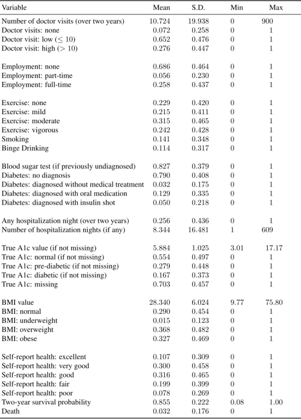
My empirical investigation of the contributors to preventive testing behavior is applied to blood sugar screening and diabetes risks. The HRS provides important information necessary for assess-ing an individual’s probability of havassess-ing a blood sugar test, includassess-ing the number of doctor visits and nights of hospitalization, blood sugar testing and test results. The summary statistics for the key variables are in Table 4.2.
Table 4.2: Summary statistics for endogenous variables
Variable Mean S.D. Min Max
Number of doctor visits (over two years) 10.724 19.938 0 900
Doctor visits: none 0.072 0.258 0 1
Doctor visit: low (≤10) 0.652 0.476 0 1 Doctor visit: high (>10) 0.276 0.447 0 1
Employment: none 0.686 0.464 0 1
Employment: part-time 0.056 0.230 0 1 Employment: full-time 0.258 0.437 0 1
Exercise: none 0.229 0.420 0 1
Exercise: mild 0.215 0.411 0 1
Exercise: moderate 0.315 0.465 0 1
Exercise: vigorous 0.242 0.428 0 1
Smoking 0.141 0.348 0 1
Binge Drinking 0.114 0.317 0 1
Blood sugar test (if previously undiagnosed) 0.827 0.379 0 1 Diabetes: no diagnosis 0.790 0.408 0 1 Diabetes: diagnosed without medical treatment 0.032 0.175 0 1 Diabetes: diagnosed with oral medication 0.129 0.335 0 1 Diabetes: diagnosed with insulin shot 0.050 0.218 0 1 Any hospitalization night (over two years) 0.256 0.436 0 1 Number of hospitalization nights (if any) 8.344 16.481 1 609 True A1c value (if not missing) 5.884 1.025 3.01 17.17 True A1c: normal (if not missing) 0.554 0.497 0 1 True A1c: pre-diabetic (if not missing) 0.279 0.448 0 1 True A1c: diabetic (if not missing) 0.167 0.373 0 1
True A1c: missing 0.703 0.457 0 1
BMI value 28.340 6.024 9.77 75.80
BMI: normal 0.290 0.454 0 1
BMI: underweight 0.015 0.123 0 1
BMI: overweight 0.368 0.482 0 1
BMI: obese 0.327 0.469 0 1
Self-report health: excellent 0.107 0.309 0 1 Self-report health: very good 0.300 0.458 0 1 Self-report health: good 0.316 0.465 0 1 Self-report health: fair 0.199 0.399 0 1 Self-report health: poor 0.078 0.269 0 1 Two-year survival probability 0.855 0.222 0.08 1.00
question is skipped in the survey as individuals with diabetes are instructed to regularly monitor their blood sugar levels. Among the undiagnosed person-wave observations, the average blood sugar test rate in a two-year period is 0.827. I also observe the self-reported diagnosis outcome if the individual is diagnosed with diabetes from the diabetes stage questions in HRS: “Has a doctor ever told you that you have diabetes or high blood sugar?”, “In order to treat or control your diabetes, are you now taking medication that you swallow?” and “Are you now using insulin shots or a pump?”. The diabetes stages show that 79 percent of person-wave observations are not diagnosed with diabetes, 3.2 percent are diagnosed with diabetes but do not have any medical treatment, 12.9 percent are diagnosed with diabetes and take some oral medications, and 5 percent are diagnosed with diabetes and treated with insulin shots.
I observe an individual’s true A1c value from the HRS linked bio-marker data set every four years. Among the observed values, the average A1c is 5.884. Based on medical guidelines, I define those with A1c values lower than 5.7 to have normal levels, those with A1c values between 5.7 and 6.4 to be pre-diabetic, and those with A1c values higher than 6.4 to be diabetic. Accordingly, 55.4 percent of the non-missing estimation sample have A1c readings in the normal range, 27.9 percent have A1c readings in the pre-diabetic range, and 16.7 percent have A1c readings in the diabetic range.
The average number of doctor visits (over a two-year period) is 10.724 with 7.2 percent of observations having no doctor visits. Regarding nights in hospitals, 74.4 percent of person-wave observations have no hospital nights (over a two-year period). Among those who have any hospital nights, the average number of hospital nights is 8.344.
4.3 Lifestyle behaviors
Because diabetes prevention includes lifestyle behaviors, I also desire information on body mass and nutrition, exercise, smoking, and drinking behaviors (Table 4.2).
observe nutrition (or diet) behavior from the HRS. While the diet and nutrition information could potentially be reflected by the BMI evolution after conditioning on the level of exercise.
In the HRS, exercise information is collected using three questions about the frequencies of vigorous, moderate and mild exercise. The responses include 5 categories: (1) everyday, (2) more than once a week, (3) once a week, (4) one to three times a month, and (5) hardly ever or never. I group (1) and (2) as high level, (3) and (4) as low level, and (5) as never, for each type of exercise. To simplify the exercise level measures, I construct an aggregate exercise variable based on frequencies of each type of exercise.5 In the sample, 22.9 percent of observations have no
exercise, 21.5 percent have mild level of exercise, 31.5 percent have moderate exercise and 24.2 percent have vigorous exercise. I also observe smoking and drinking behaviors: 14.1 percent of person-wave observations are observed to smoke and 11.4 percent are observed to binge drink, which is defined as having 4 or more drinks in at least one day in the past three months.
4.4 Perception of health
Since individuals may make decisions using imperfect information about own health, some information about the individual’s perception about health is required. I observe the individual’s self-reported health status and subjective survival probability in the HRS (Table 4.2).
The self-reported health status contains five categories: excellent, very good, good, fair, and poor. Almost a third of observations report good health status, 10.7 percent report excellent, 30.0 percent report very good, 19.9 percent report fair, and only 7.8 percent report poor. Based on the longevity expectation questions collected by HRS, a subjective two-year survival probability is calculated for each person-wave observation using the method in Wang (2014) and Perozek (2008). 4.4.1 Calculation of subjective survival probability
The HRS collects two questions about expected longevity: (1) “What is the percent chance that you will live to be 75 or more?” and (2) “What is the percent chance that you will live 10
5Specifically, different alternatives are modeled as: no exercise includes low/never mild exercise, never/low
more years (to be age [85/80/90/95/100] or more)?” Following Wang (2014), I translate these two longevity questions to a two-year subjective survival probability. The reason is threefold. First, it is difficult to evaluate the raw longevity expectation across individuals with different ages. For example, the expectation to live to age 80 for a 60 years old respondent is not comparable to that for a 70 years old respondent. Second, the method combines information from two observed subjective longevity expectations in one measure. Third, this method also addresses rounding and measurement error issues in the reported longevity probabilities (Manski and Molinari, 2010). I describe the method in more detail in this section.
First, a hazard function with a Weibull distribution is used to model a respondenti’s subjective survival curve at period t. Her two-year survival probability is inferred from the curve (Wang, 2014). That is, a respondenti’s true subjective expectation to survive anothersyears at periodtis:
ptit(s) =exp(−(γits)kit)
wherekitis shape parameter andγitis scale parameter. Accordingly, the true subjective expectation to live to age 75 and 85 are:
ptit(st,75) =exp(−(γitst,75)kit) (4.1)
ptit(st,85) =exp(−(γitst,85)kit) (4.2)
wherest,75andst,85are years from the interview date (or periodt) to age 75 and 85 for individual
i, respectively. The shape and scale parameters can be identified if observept
it(st,75)andptit(st,85).
Specifically,kitis identified as:
ln[ln[p
t
it(st,75)]
ln[pt
it(st,85)]
] =ln[s
kit t,75
skitt,85] =kitln st,75
st,85
kit =ln[ ln[pt
it(st,75)]
ln[pt
it(st,85)]
]/ lnst,75 st,85
γit is identified by plugging identifiedkit back to equation (4.1) or (4.2). After identifyingkit
tusing
ptit(2) =exp(−(γit2)kit)
One issue of this method is that it requires me to observe at least two expected longevity probabilities for each person-wave observation. However, for those who are older than 65 years old, the HRS stops collecting their first longevity probability (i.e., the subjective probability of living to age 75 or more). Aa a result, I observe only one longevity probability for this group of respondents in my research sample. On method to address this problem is to drop observations who are older than 65 years old, but this makes me drop half of my estimation sample. Alternatively, I propose that this issue can be addressed using a method in Perozek (2008) to calculate/impute an additional subjective longevity probability using the observed subjective longevity probability from the HRS and an objective survival probability from the Social Security Area (SSA) life table (Bell and Miller, 2016). The SSA life table contains gender-age specific survival probabilities for each age (ranging from 0 to 119) and updates every ten years.6 Specifically, the additional
subjective probability of living to age y, conditional on the individual i is alive in period t with current ageageit(Pit(y|ageit)) is calculated as:
Pi(y|ageit) =Pg(y|85, ageit)∗Pi(85|ageit) (4.3)
wherePi(85|ageit)is the observed self-reported survival probability to age 85 conditional on being alive at current ageageitfrom the HRS, andPg(y|85, ageit) =Pg(y|85)is the SSA life table gender specific probability of an individualiwith genderg living to ageyconditional on surviving to age 85. In practice, I calculate the second subjective longevity probability to a target age that is ten more years than the one used in the HRS longevity expectation question for each individual. For example, if HRS collects the subjective longevity expectation to age 90, I calculate the additional subjective longevity probability to age 100. With this additional longevity probability, I estimate the shape and scale parameters (i.e.,γiandkit) in equation 4.1 and 4.2.
Second, to address the rounding and measurement error issue, an interval response approach is employed following Wang (2014), Manski and Molinari (2010), and Hudomiet et al. (2011). The interval response approach does not rely on the actual value of reported subjective probability, which may subject to rounding or measurement errors. Instead, it uses a corresponding interval to identify the shape and scale parameters. Specifically, I assume that each reported longevity probability of individuali(e.g.,pit(st,85)) is in a pre-specified interval[Lit,st,85, Uit,st,85]. The true
subjective longevity probability (e.g.,pt
it(st,85)) is in the same interval, but is not necessarily equal
to the reported one due to rounding or measurement error. In practice, I allow the true subjective longevity probability to lie anywhere within the interval and identify corresponding sets of γit and kit.7 Each set of kit and γit is used to calculate a subjective two-year survival probability, pt
it(2), and the average value of all calculatedptit(2)is used as the two-year survival probability for individualiin periodt.
For respondents who are 90 years old or older, because the HRS stops collecting any subjective longevity expectations among them, I use the SSA life-table gender specific two-year survival probabilities to fill in.
4.5 Employment
Employment behavior also determines income and available time for preventive care. I observe different employment statuses in the HRS (Table 4.2). In the estimation sample, 68.6 percent of individual-wave observations are not working, including those who are retired and those who are unemployed. This high rate of non-employment reflects that a majority of the individuals in the estimation sample are approaching or past retirement age. There are 5.6 percent of observations working part-time and 25.8 percent working full-time.
4.6 Personality measures and exogenous characteristics
Lastly, I observe pessimism in the HRS, which is used to identify health anxiety. Since the pilot survey in 2004, the HRS has included a psychosocial and lifestyle questionnaire in each
7Specifically, each interval is discretized into 10 cells. The middle point of each cell for the first longevity
probabil-ity (e.g.,pt
it(st,75)) is matched with the middle point of each cell for the second longevity probability (e.g.,ptit(st,85))