RECONSTRUCTING MODERN AND PLIOCENE (C. 5.4-2.4 MA) DECADAL CLIMATE VARIATIONS IN THE PALEOENVIRONMENTS OF THE MIDDLE ATLANTIC BIGHT USING ISOTOPE AND INCREMENT SCLEROCHRONOLOGY
Joel Wayne Hudley
A dissertation submitted to the faculty of the University of North Carolina at Chapel Hill in partial fulfillment of the requirements for the degree of Doctor of Philosophy in the Department of Geological Sciences
Chapel Hill 2012
iii ABSTRACT
JOEL W. HUDLEY: Reconstructing modern and Pliocene (c. 5.4-2.4 Ma) decadal climate variations in the paleoenvironments of the Middle Atlantic Bight using isotope
and increment sclerochronology (Under the direction of Donna Surge) Ocean characteristics on geologic timescales are poorly understood, have varied in the past, and are critical to understanding how the ocean may respond to future human-induced climate change. Recent climate studies have identified that environmental
variations in the Mid-Atlantic Bight (MAB) are related to larger global climate variations throughout the Late Cenozoic such as the Atlantic meridional overturning circulation pattern and ocean-atmospheric teleconnections. Modern physical oceanographic studies in the MAB using the modern instrument records show high interannual variability with longer, multi-decadal warming trends. The goal of this investigation is to reveal annual to multi-decadal variations in sea surface temperatures of the MAB during the Pliocene (5.4-1.8 Million years ago (Ma). This investigation employs isotope and increment records from marine bivalves as proxies for ocean bottom temperature in conjunction with a basic understanding of the modern physical oceanographic flow model along the Atlantic continental shelf.
iv
v
ACKNOWLEDGEMENTS
vii
TABLE OF CONTENTS
TABLE OF CONTENTS ... VII
LIST OF TABLES ... X
LIST OF FIGURES ... VIII
LIST OF ABBREVIATIONS AND SYMBOLS ... IX
CHAPTER 1: INTRODUCTION, PURPOSE, DISSERTATION ORGANIZATION . 10
1.1INTRODUCTION ... 10
1.2RESEARCH PURPOSE ... 14
1.3DISSERTATION ORGANIZATION ... 15
LITERATURECITED ... 19
CHAPTER 2: BACKGROUND ... 23
2.1PURPOSE ... 23
2.2BACKGROUND ... 25
2.2.1 Physical Geographic Setting... 25
2.2.2 Sedimentology ... 31
2.2.3 Oceanographic Setting... 32
2.2.4 Geologic Setting and Stratigraphy... 36
vii
2.3. CONCLUSIONS ... 40
REFERENCES ... 42
CHAPTER 3: ADDRESSING THE SINGLE COUNTER PROBLEM USING A COMPUTER-ASSISTED IMAGE AGING METHOD ... 57
3.1 INTRODUCTION... 58
3.2 MATERIALS AND METHODS ... 60
3.2.1 Materials ... 60
3.2.2 Visual aging method ... 62
3.2.3 Computer-assisted aging ... 63
3.2.4 Comparison of aging methods ... 65
3.3 RESULTS ... 66
3.3.1 Visual aging ... 66
3.3.2 Computer-assisted aging ... 66
3.3.3 Comparison of aging methods ... 67
3.3.4 Other Bivalve Proxy Results ... 68
3.4 DISCUSSION ... 69
3.5. CONCLUSIONS ... 70
ACKNOWLEDGEMENTS ... 71
REFERENCES ... 72
CHAPTER 4: COMPARATIVE SCLEROHRONOLOGY OF MODERN AND PLIOENE SURF CLAM (MACTRIDAE) ALONG THE WESTERN MID-ATLANTIC: THE ARCHETYPE REVISITED... 79
viii
4.1.1 ECOLOGY OF MODERN ATLANTIC SURF CLAM ... 83
4.1.2 MODERN LOCATION ... 85
4.1.3 GEOLOGIC CONTEXT ... 87
4.2 MATERIALS AND METHODS ... 88
4.2.1 COLLECTION AND GROWTH INCREMENTS ... 88
4.2.2 STABLE ISOTOPES ... 93
4.3 RESULTS ... 97
4.3.1 SHELL AGES AND GROWTH PARAMETERS ... 97
4.3.2 VARIATIONS IN GROWTH INCREMENTS ... 97
4.3.3 VARIATIONS IN STABLE ISOTOPES ... 98
4.4 DISCUSSION ... 100
4.4.1 COMPARISON OF GROWTH PARAMETERS ... 100
4.4.2 SGI COMPARISONS ... 104
4.4.3 SPECIES STABLE ISOTOPE DISTINCTIONS ... 106
4.5 CONCLUSIONS ... 110
ACKNOWLEDGEMENTS ... 110
REFERENCES ... 112
CHAPTER 5: IN SEARCH OF LONG-LIVED BIVALVES FROM THE PLIOCENE MID-ATLANTIC: STABLE ISOTOPE AND INCREMENT ANALYSIS OF LARGE MARINE BIVALVES, VIRGINIA & NORTH CAROLINA, U.S.A ... 141
5.1 INTRODUCTION... 142
ix
5.3 METHODS ... 148
5.3.1 Fossil bivalve shell preparation and growth increment reading ... 148
5.3.2 Isotope sclerochronology ... 150
5.3.3. Temperature estimates ... 151
5.3.4 Growth analysis ... 152
5.3.5 Increment analysis ... 154
5.3.6 Spectral analysis ... 155
5.4 RESULTS ... 157
5.4.1 Isotope sclerochronology ... 157
5.4.2 Aging ... 159
5.4.3 Growth models ... 160
5.4.4 Increment analysis ... 160
5.4.5 Spectral analysis ... 161
5.5 DISCUSSION ... 162
5.5.1 Oxygen Isotope ratios in Panopea ... 162
5.5.2 Interpretations of paleotemperature estimates from Glycymeris ... 164
5.5.3 G. americana as a multi-decadal climate archive. ... 169
5.6. CONCLUSIONS ... 172
ACKNOWLEDGMENTS ... 173
APPENDIX A: SPISULA ... 189
APPENDIX B: GLYCYMERIS AND PANOPEA ... 246
x
LIST OF TABLES
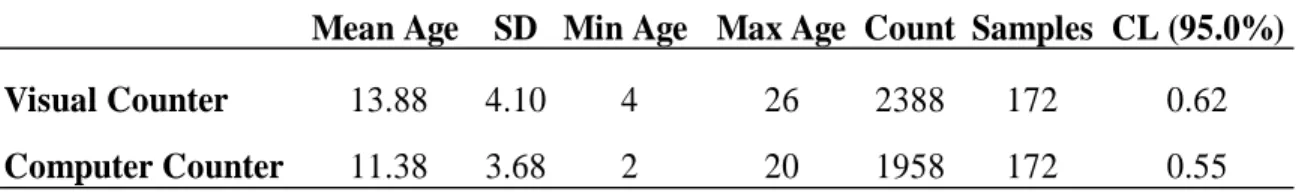
Table 3.1 Descriptive statistics of the Visual and Computer counters. ... 78 Table 4.2. VBGM parameters from natural populations of modern and fossil Spisula along the Atlantic coast of the United States. ... 120 Table 4.3. Isotopic composition of shells. Samples taken from the Spisula were micro-milled from the chondrophore. Samples were run at the University of Arizona's
Environmental Isotope Laboratory ... 121 Table 4.4. Summary statistics for δ18O, δ13C, and δ18
O based temperature estimates preserved in modern and Mid-Pliocene aged Spisula shells. Temperature estimates calculated using the equation reported by Schöne et al. (2005) as modified from
Grossman and Ku (1986). ... 126 Table 4.5. Standardize growth indices (SGI) from around the New York Bight and along the New Jersey shore with sample depth (S.D.) ... 128 Table 4.6. Standardize growth indices (SGI) from off the Delmarva peninsula and
viii
LIST OF FIGURES
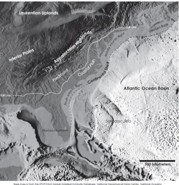
Figure 2.1. Physical Setting of eastern North America and the western Atlantic Ocean
Basin. ... 50
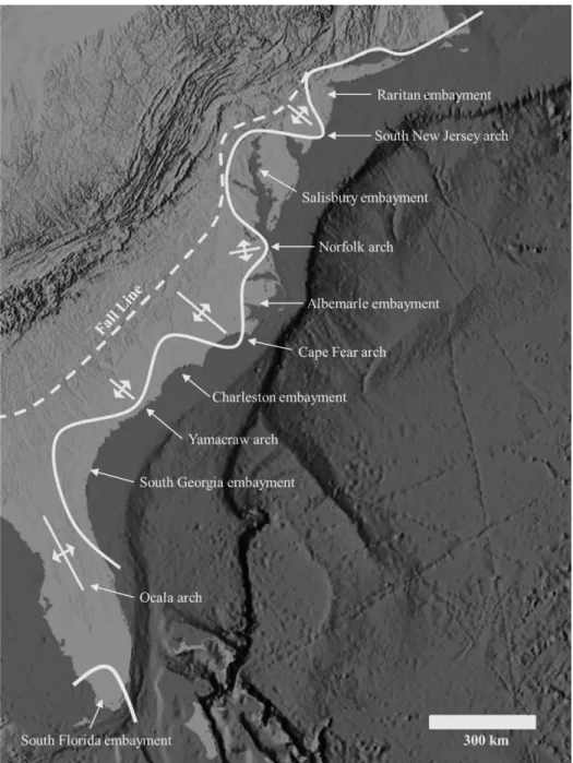
Figure 2.2 Generalized onshore embayment and major structural features map othe Atlantic Coastal Plain (after Ward et al., 1991). ... 51
Figure 2.3. Schematic map and cross-section of the eastern North American coastal plain and western Atlantic basin. ... 52
Figure 2.4. Filled contour map showing the percent sand-sized sediment along the eastern North American continental shelf and slope. ... 53
Figure 2.5. Pliocene stratigraphic nomenclature for the coastal plain of a combined North Carolina and Virginia.. ... 54
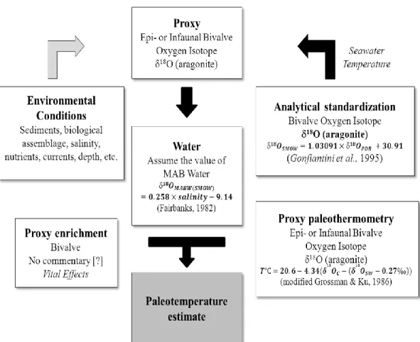
Figure 2.6. Flow chart showing the conventional methods employed in isotope paleothermometry. ... 55
Figure 2.7 Bivalves examined for this study. ... 56
Figure 3.1. Collection localities for Spisula spp. collected alive on the continental shelf, and Pliocene fossil specimens collected from coastal plain deposits. ... 75
Figure 3.2. Example comparison of visual count versus computer-assisted count picks on sample number 6321621994. ... 76
Figure 3.3. Age-bias plot. Counter age versus average test age. ... 77
Figure 4.1 Collection localities for modern and Pliocene specimens. ... 130
Figure 4.2 Example of how Spisula shells were measured and sectioned. ... 131
Figure 4.3 Graph of valve length versus chondrophore length ... 132
Figure 4.4 Plot comparing von Bertalanffy growth model parameters k and L∞ of MAB and MACP Spisula arranged by species and region ... 133
Figure 4.5 Oxygen and carbon isotopic profiles from Spisula solidissima specimens and S. s. similis specimen ... 134
Figure 4.6 Temperature (ºC) estimates for Spisula S. s. solidissima and S. s. similis specimens. ... 135
ix Figure 4.8 Covariance of δ18O and δ13
C values from modern Spisula spp. and Pliocene S. confraga. ... 137 Figure 4.9 Oxygen and carbon isotopic profiles from S. confraga specimens ... 138 Figure 4.10 Temperature (ºC) estimates for S. confraga specimens ... 139 Figure 4.11 Comparison of individual and all annual standardized growth indices) to mean annual temperature and salinity index. ... 140 Figure 5.1. Location of collection sites along the Middle Atlantic Coastal Plain. ... 178 Figure 5.2 Shells of Glycymeris americana and Panopea reflexa cut through the axis of maximum growth to show annual growth increments. ... 179 Figure 5.3 Variation of δ18O and δ13C values (‰ VPDB) versus distance (in millimeters)
from the umbo to the ventral edge in shells of G. americana (GLY-A & -C).. ... 180 Figure 5.4 Variation of δ18O and δ13C values (‰ VPDB) versus distance from the umbo
to the ventral edge in cardinal tooth of P. reflexa (PR-C & -D). ... 181 Figure 5.5 Histogram: Age versus frequency plot of Yorktown and Chowan River
Formation G. americana populations ... 182 Figure 5.6 Growth model comparison ... 182 Figure 5.7 Temperature estimates (ºC) versus distance (in millimeters) from the umbo to the ventral edge of the cardinal tooth in P. reflexa (PR-C & -D) shells. ... 183 Figure 5.8 Temperature estimates (ºC) versus distance (in millimeters) from the umbo to the ventral edge of G. americana (GLY-A & -C) valves.. ... 184 Figure 5.9 Spectral densities for four time series as computed by the SSA-MTM method. (log10 y-axis scale versus frequency on the x-axis). ... 185
Figure 5.10 Spectral densities for Yorktown SGI time series as computed by the SSA-MTM method.. ... 187 Figure 5.11 Spectral densities for Chowan River time series as computed by the SSA-MTM method. ... 188
LIST OF ABBREVIATIONS AND SYMBOLS 1. ± plus or minus
2. ‰ per mil or parts per thousand 3. 13C carbon isotope 13
4. 14C radiocarbon isotope 14 5. 18O oxygen isotope 18 6. A. islandica Arctica islandica
7. AMS accelerator mass spectrometry 8. cm centimeter
9. DIC dissolved inorganic carbon 10.et al. and others
11.GBS Georges Bank-Scotian Shelf
12.GI Growth index
13.G. americana Glycymeris americana 14.G. glycymeris Glycymeris glycymeris 15.HCO3
−
bicarbonate 16.i.e., that is
17.MAB Middle Atlantic Bight
18.MACP Middle Atlantic Coastal Plain
19.MPWP Mid Pliocene Warm Period
20.mm millimeter
21.NBS National Bureau of Standard
22.NOAA National Oceanographic and Atmospheric Agency 23.oC degrees Celsius
24.P. abrupta Panopea abrupta 25.P. reflexa Panopea reflexa 26.psu practical salinity units
27.RWI Ring width index
28.S. confraga Spisula confraga 29.S. modicello Spisula modicello
30.S. s. similis Spisula solidissima similis 31.S. s. solidissima Spisula solidissima
32.SGI Standardized growth index
33.SHW Shelf Water
34.SLW Slope Water
35.spp. Species pluralis or Genus, species unidentified 36.SST sea surface temperature
37.T temperature
38.USGS United States Geological Survey
39.VBGM Von Bertalanffy growth model
40.VPDB Vienna Pee Dee Belemnite
41.VMNH Virginia Museum of Natural History
42.VSMOW Vienna Standard Mean Ocean Water 43.δ 13C carbon isotope ratio
x
45.δ 18OW oxygen isotope ratio of water
46.α13C carbon isotope 13 fractionation factor
CHAPTER 1: INTRODUCTION, PURPOSE, DISSERTATION ORGANIZATION 1.1 Introduction
The Intergovernmental Panel on Climate Change (IPCC) projects a future warmer climate through the 21st century (IPCC WG1,2007). The predicted increase in air temperature is related to the observed and forecasted increases in anthropogenic
greenhouse gases. The potential effects of a future warmer climate include sea level rise, extreme weather events, migrating ecosystems, and changing resources. Climate
scientists and policy makers responsible for making decisions on the mitigation of and adaptation to human-induced climate change have determined that understanding past warm climate states is critical to evaluate its response to increasing greenhouse gas concentrations (IPCC WG1, 2007). Determining mitigation and adaptation strategies to lessen the resulting worldwide socio-economic stresses requires efforts to reduce the uncertainties associated with the nature and rate of projected climate change (IPCC, 2007; Robinson and Dowsett, 2010). To reduce the uncertainties, geologists and paleoclimatologists use proxy records to extend the instrumental record and study analogs to projected future warm climate.
11
improvement in the networks of available proxy data sets that can be used to develop spatial maps (with associated errors) for each season of the last few millennia is essential (Jones and Mann, 2004). There is a need to develop high-resolution reconstructions as templates for calibrating the longer, lower resolution proxy data networks. To achieve this goal, reliable proxies must be “calibrated” and independently “validated” against instrumental records. Tree rings and coral isotopic data are currently the most widespread sources of annually and sub-annually resolved proxies, but both proxies are limited in spatial and temporal coverage. Early successes in the development of annual
chronologies using the long-lived bivalve Arctica islandica (Wiedman and Jones, 1994) demonstrate that molluscan shell records are effective high-resolution proxy indicators that can potentially serve as useful data sets to develop multi-proxy climate
reconstructions.
Over the last 30 years, many scientific papers have asserted that intervals in Earth history can be used as an analogue for future climate change. To be considered an appropriate analogue, the warm climate interval must result from increased
concentrations of atmospheric greenhouse gases due to a transient forcing and have similar regional and global climate patterns due to continental configuration and orogenic effects. Studies of potential analogues have focused on warm intervals during the
12
The warm intervals of the Quaternary (early Holocene and the Pleistocene
interglacials) all have the same position of continents and mountain ranges. However, evidence from trace gas records in ice cores indicate that atmospheric concentrations of CO2 are already higher than at any time during the last 800,000 years (Siegenthaler et al.,
2005; Loulergue et al., 2008). Evidence from new alkenone-based, boron isotope-based and stomatal density-based CO2 proxy data indicate that the current concentration of CO2
(394.45 ppm recorded in 2012; data from the National Oceanic and Atmospheric
Administration’s (NOAA) Earth System Research Laboratory, Mauna Loa Observatory) in the atmosphere may not have been reached in the last 3 million years. There is oceanic and terrestrial evidence for a transient forcing-induced warming during the Paleocene-Eocene Thermal Maximum (PETM) (Kennett and Stott, 1991; Zachos et al., 2005). However, the rate of climatic and ocean geochemical change is likely to have been an order of magnitude slower (Rigwell, 2007; Zeebe et al., 2009) and the configurations of continents, ocean gateways, and orogenic belts are widely dissimilar for intervals in Earth history earlier than the late Miocene (23.3-5.3 Ma). The search for an appropriate
analogue of future global warming continues even though research concluded that no satisfactory warm intervals in Earth history could be used as a frame of reference or even a possible analogue for future atmospheric CO2-induced warming (Crowley, 1991;
Haywood et al., 2011).
13
al., 2011). The Pliocene was remarkably similar to modern climate when compared to other geologically recent warm intervals in terms of positions of the continents, the thermal isolation of Antarctica (Zachos et al., 2001), and atmospheric CO2 concentrations
(Haywood et al., 2009). Even so, Pliocene interglacials reflected long-term equilibrium for a given ambient CO2 level following the long-term negative trend in atmospheric CO2
through the Cenozoic and not a rapid transient forcing on climate (Haywood et al., 2011). Evidence from faunal-based transfer functions and isotopic proxies of paleotemperature show the MPWP was approximately 2-3ºC warmer than today (Robinson et al., 2008). Moreover, the spatial distribution of global sea surface temperature (SST) during the MPWP was different from today because northern high latitudes were warmer, while temperatures in the tropics were similar (Dowsett et al., 2010; Federov et al., 2006).
General circulation models (GCM) using MPWP boundary conditions produce surface temperature anomalies in the range of late twenty-first century climate
projections (Haywood et al., 2001). Still, discrepancies exist between proxy evidence and GCM simulations (Dowsett et al., 2009). For example, hypotheses for both permanent El Niño and La Niña conditions have been modeled and documented in alkenone-based SST reconstructions (Lawrence et al., 2006; Dowsett and Robinson, 2010). A Pliocene climate dominated by either permanent state is significantly different from modern climate
14
provide SST variability at a resolution capable of testing the environmental response to interannual atmospheric/oceanic phenomena.
1.2 Research Purpose
The purpose of this dissertation is to develop and employ classic and new high-resolution bivalve proxy records to reconstruction oceanic conditions in the near and distant past. In this series of studies, high-resolution records from live-collected clams from the Mid Atlantic Bight (MAB) and fossil Pliocene bivalves from fossiliferous units along the US Mid Atlantic Coastal Plain (MACP) are examined and compared to modern instrument records. High-resolution data sets recorded in bivalve shells are more
analogous to instrumental observations than fossil assemblage data. Comparing modern climate records to Pliocene data series is necessary to better constrain uncertainties of future climate prediction. The estimation and comparison of past sea water temperatures to modern records allow the study of other larger questions about global warming
intervals, such as: (1) are significant changes in interannual variability experienced along the western Mid Atlantic Shelf; (2) are there shifts in the boundaries of shelf province waters due to these changes; and (3) are past natural (pre-industrial) ocean-atmospheric interactions similar to baseline anthropogenically-altered modern analogues.
15
into the Pleistocene. While previous research has examined Pliocene SST variation and seasonality in MACP deposits, little is known about interannual variability in the Pliocene and how it compares to present conditions. Interannual variability of modern SST in the MAB is related to a combination of local atmospheric processes and advection of water masses into the shelf area (Mountain, 2003). Warmer SST in the Pliocene may result from more frequent and northern penetration of warm water masses, a decline in the influence of northern cold waters, and/or different tropical perturbations to
atmospheric circulation.
Much warmer winter SST during the Pliocene indicates reduced seasonality in MACP shelf waters, suggesting more stable warming mechanisms and diminished interannual variability (Krantz, 1990; Cronin, 1991). However, this scenario conflicts with colder winter and summer MPWP temperatures and a larger seasonal range in Virginia
(Goewert and Surge, 2008). A more likely scenario is that winter SST along the MACP was warmer, but that the large interannual variability exhibited in the modern MAB also existed in the Pliocene. This hypothesis agrees with observed faunal data from the MACP. A reconstruction of interannual to decadal trends in SST provides evidence to test the validity of previously conflicting results.
1.3 Dissertation Organization
16
change along the coastal shelf regions of the eastern United States. This research is based on modern analog techniques. All methods and data are compared to instrumental data from the late Holocene, but the overall goal is investigating the climate of the Pliocene (5.4-1.8 Million years ago (Ma)). The MACP is an ideal location for this research. The present MAB shelf is well instrumented, and the modern bivalve proxies are well studied due to commercial exploitation. Also, MACP shell beds contain numerous
well-preserved molluscs and well-documented biostratigraphy and chronology. This work provides much needed proxy data for models attempting to reconstruct environmental and climatic changes in shallow marine settings along the low to mid-latitudal gradient of the western Atlantic shelf and those evaluating the response of regional teleconnections such as North Atlantic Oscillation.
Chapter 2 provides the background to the dissertation. This includes a brief review of the geologic history and large physiographic provinces of the eastern United States, modern oceanographic setting, and instrumental records and studies used to examine average and anomalous climate conditions in and along the MAB. A review of the North Carolina and Virginia fossil beds is also provided. Chapter 2 details the known ecology of the selected bivalve proxies, basic sclerochronological methods and assumptions, and previous works using growth increment and/or isotopic methods to investigate these proxies.
17
means of computer-assisted quality control. Age determination for live-caught bivalves is simple, but labor intensive if there is a large number of samples. Good practices assume that each sample must be examined by several readers, several times for age determination to be considered accurate, and thus requires time. This challenge is addressed by using a novel image analysis-based method of discriminating annual increments in the shell.
Chapter 4 is a reexamination of the infaunal bivalve species Spisula (Hemimactra) solidissima (Dillwyn, 1817), the archetype for contemporary increment and isotope sclerochronology experiments. S. s. solidissima studies by Jones (1983) set standard sclerochronological practices that remain unchanged, but the potential applications expressed in those earlier works are currently possible with the expanded number and range of new S. (s). solidissima specimens. Using isotope sclerochronology, this work investigates the periodicity of growth intervals in the species S. s. solidissima, S. s. similis (Say, 1822), and S.(Hemimactra) confraga (Conrad, 1833)(Pliocene), and estimates paleoenvironmental conditions during the Recent and the Pliocene using isotope and increment comparisons to instrumental records. These data increase our knowledge of Pliocene climate along the MACP, and are compared to modern environmental
conditions.
18
19 LITERATURE CITED
Chandler, M., D. Rind, and R. Thompson. (1994). Joint investigations of the middle Pliocene climate: II. GISS GCM Northern Hemisphere. Global Planetary Change, 9:197-219.
Cronin, T.M. (1991). Pliocene shallow water paleoceanography of the North Atlantic Ocean based on marine ostracodes. Quaternary Science Review, 10: 175-188.
Crowley, T. J. (1991). Are there any satisfactory geologic analogs for a future greenhouse warming. Journal of Climatology. 3, 1282–1292.
Dowsett, H. J., Robinson, M., Haywood, A. M., Salzmann, U., Hill, D. J., Sohl, L., Chandler, M. A., Williams, M. Foley, K. and Stoll, D. (2010). The PRISM3D paleoenvironmental reconstruction. Stratigraphy, 7, 123–139.
Dowsett, H.J., M.A. Chandler, T.M. Cronin, and G.S. Dwyer. (2005). Middle Pliocene sea surface temperature variability. Paleoceanography, 20: 1-8.
Dowsett, H.J., J.A. Barron, R.Z. Poore, R.S. Thompson, T.M. Cronin, S.E. Ishman, and D.A.Willard. (1999). Middle Pliocene paleoenvironmental reconstruction: PRISM2. U.S.Geological Survey Open File Report, 99-535: 1-33.
Dowsett, H.J. and R.Z. Poore. (1991). Pliocene sea surface temperatures of the North Atlantic Ocean at 3.0 Ma. Quaternary Science Review, 10: 189-204.
Dowsett, H.J. and T.M. Cronin (1990). High eustatic sea level during the middle Pliocene: Evidence from the southeastern U.S. Atlantic Coastal Plain. Geology, 18: 435-438.
Fedorov, A. V., Brierley, C. M. & Emanuel, K. (2010). Tropical cyclones and permanent El Niño in the early Pliocene epoch. Nature , 463, 1066–1070.
Fedorov, A. V., P. S. Dekens, M. McCarthy, A. C. Ravelo, P. B. deMenocal, M. Barreiro, R. C. Pacanowski, and S. G. Philander, (2006). The Pliocene paradox (mechanisms for a permanent El Niño). Science, 312, 1485–1489.
Goewert, A.E. and D. Surge. (2008). Seasonality and growth patterns using isotope sclerochronology in shells of the Pliocene scallop, Chesapecten madisonius. Geo-Marine Letters 28: 327–338.
20
Haywood, AM, Ridgwell, A, Lunt, DJ, Hill, DJ, Pound, MJ, Dowsett, HJ, Dolan, AM, Francis, JE and Williams, M (2011). Are there pre-Quaternary geological analogues for a future greenhouse warming? Philos. Trans. R. Soc. A-Math. Phys. Eng. Sci., 369, 1938.
Haywood, A. M., Chandler, M. A., Valdes, P. J., Salzmann, U., Lunt, D. J. &
Dowsett, H. J. (2009). Comparison of Mid-Pliocene climate predictions produced by the HADAM3 and GCMAM3 general circulation models. Glob. Planet. Change, 66, 208–224.
Haywood, A.M., Valdes, P.J., Sellwood, B.W., Kaplan, J.O. Dowsett, H.J. (2001). Modelling Middle Pliocene warm climates of the USA. Palaeontologia Electronica, v.4, art.5. (available at: http://palaeo electronica.org/2001_1/climate/issue1_01.htm) Haywood, A.M., P.J. Valdes, and B.W. Sellwood. (2000). Global scale palaeoclimate reconstruction of the middle Pliocene climate using the UKMO GCM: initial results. Global and Planetary Change, 25: 239-256
International Panel on Climate Change (2007), Climate change 2007: The physical science basis. In Contribution of Working Group I to the Fourth Assessment Report of the Intergovernmental Panel on Climate Change (eds S. Solomon, D. Qin, M. Manning, Z. Chen, M. Marquis, K. B. Averyt, M. Tignor & H. L. Miller). Cambridge, UK: Cambridge University Press.
Jones, D.S. and I.R. Quitmyer. (1996). Marking time with bivalve shells: oxygen isotopes and season of annual increment formation. Palaios, 11: 340-346.
Jones, D.S. (1983). Sclerochronology: reading the record of the molluscan shell. American Scientist, 71: 384-391.
Jones, D.S., D.F. Williams, and M.A. Arthur (1983). Growth history and ecology of the Atlantic surf clam Spisula solidissima (Dillwyn), as revealed by stable isotopes and annual shell increments. J. Exp. Mar. Biol. Ecol., 13: 225-242.
Jones, D.S. (1981). Annual growth increments in shells of Spisula solidissima record marine temperature variability. Science, 211, 4478: 165-167.
Jones, D.S. (1980). Annual cycle of shell growth increment formation in two
continental shelf bivalves and its paleoecologic significance. Paleobiology, 6(3): 331-340.
Jones, D.S., I. Thompson, and W. Ambrose (1978). Age and growth rate
21
Jones, P.D., K.R. Briffa, T.P. Barnett and S.F.B. Tett (1998). High-resolution palaeoclimate records for the last millennium: interpretation, integration and
comparison with General Circulation Model control-run temperatures. The Holocene, 8(4). 455-471
Jones, P. D., and M. E. Mann (2004), Climate over past millennia, Rev. Geophys., 42, RG2002
Krantz, D.E. (1990) Mollusk-Isotope Records of Plio-Pleistocene Marine Paleoclimate, U.S. Middle Atlantic Coastal Plain. Palaios, 5: 317-335.
Kennett, J. P. and Stott, L. D. (1991), Abrupt deep-sea warming, palaeoceanographic changes and benthic extinctions at the end of the Paleocene. Nature 353, 225–229. Meehl, G.A., T.F. Stocker, W.D. Collins, P. Friedlingstein, A.T. Gaye, J.M. Gregory, Kitoh, R.Knutti, J.M. Murphy, A. Noda, S.C.B. Raper, I.G. Watterson, A.J. Weaver, Z.-C. Zhao. (2007). Global climate projections. In: S. Solomon, D. Qin, M. Manning, Z. Chen, M. Marquis, K.B. Averyt, M. Tignor, and H.L. Miller (Eds.), The Physical Science Basis. Contribution of Working Group I to the Fourth Assessment Report of the Intergovernmental Panel on Climate Change, Cambridge University Press, Cambridge, United Kingdom, and New York, NY, USA.
Lawrence KT, Liu ZH, Herbert TD (2006). Evolution of the eastern tropical Pacific through Plio-Pleistocene glaciation . Science , 312 5770:79-83
Loulergue, L. et al. 2008 Orbital and millennial-scale features of atmospheric CH4
over the past 800,000 years. Nature, 453, 383–386.
Molnar, P. and M.A. Cane. (2002). El Niῇo’s tropical climate and teleconnections as a blueprint for pre-Ice Age climates. Paleoceanography, 17: 11.1-11.12
Mountain, D. G. (2003). Variability in the properties of Shelf Water in the Middle Atlantic Bight, 1977–1999, Journal of Geophysical Research, 108(C1), 3014
Ridgwell, A. (2007). Interpreting transient carbonate compensation depth changes by marine sediment core modeling. Paleoceanography, 22, PA4102.
Robinson, M. M., Dowsett, H. J., Dwyer, G. S. & Lawrence, K. T. (2008). Re- evaluation of mid-Pliocene North Atlantic sea-surface temperatures.
Paleoceanography, 23, PA3213
Siegenthaler, U. et al. 2005 Stable carbon cycle-climate relationship during the Late Pleistocene. Science, 310, 1313–1317.
22
Weidman, C.R., Jones, G.A. and Lohmann, K.C. (1994). The long-lived mollusk Arctica islandica- A new paleoceanographic tool for reconstruction of bottom temperatures for the continental shelvs of the northern North-Atlantic Ocean. Geophys. Res.-Oceans, 99: C9, 18305.
Zachos, J. C. et al. (2005), Rapid acidification of the ocean during the Paleocene– Eocene Thermal Maximum. Science, 308, 1611–1615.
Zachos, J., M. Pagani, L. Sloan, E. Thomas, and K. Billups. (2001). Trends, rhythms, and aberration in global climate 65 Ma to present. Science, 292: 686-693.
Zeebe, R. E., Zachos, J. C. and Dickens, G. R. (2009). Carbon dioxide forcing alone insufficient to explain Palaeocene–Eocene Thermal Maximum warming. Nat. Geosci. 2, 576–580.
Zubakov, V. A. and Borzenkova, I. I. (1988). Pliocene palaeoclimates: past climates as
CHAPTER 2: BACKGROUND 2.1 PURPOSE
The study of climate in the past, present and future is essential to society This dissertation focuses on using bivalve proxies to explore aspects of climate change along the coastal shelf regions of the eastern United States. All of the methods and data are anchored in late Holocene/Anthropocene climate studies, but the overall goal is
investigating the climate of the Pliocene (5.4-1.8 Million years ago (Ma)). The Pliocene represents the last epoch before the Earth shifted completely into an icehouse world after the long Cenozoic transition from the late Mesozoic greenhouse. There is
well-documented evidence that global temperature and atmospheric CO2 levels are directly
related, and that both steadily declined through the Cenozoic. They reached their lowest levels during the Quaternary. However, in the last decades of the Holocene, atmospheric CO2 levels rose and are now projected to reach levels not present in the atmosphere since
the Pliocene.
The mechanisms driving atmospheric CO2 levels in the late Holocene are
different than the mechanisms altering atmospheric CO2 concentrations during the
Pliocene. Natural forcing mechanisms operating on timescales of thousands to millions of years forced CO2 levels to rise and fall during the Pliocene. In comparison,
24
However, some conditions during the Pliocene are similar to today or the probable near future. For example, the distribution of continents and ocean basins are in similar configurations. Estimates of mid-ocean spreading and continental collision rates are unchanged since Pliocene times, so mountain ranges are in the same locations and similar in elevation, ocean basins are similar in width, and volcanic activity is likely comparable. The physical and biological processes that sculpt our dynamic planet (insolation, wind and ocean circulation patterns, weather, erosion, respiration, photosynthesis, bioturbation, etc.) remain unchanged, though the exact biological species and topography do vary. Most importantly for society (at least for government planners), though the rate of cause and effects are different, the concentrations of CO2 and the expected temperatures are
similar.
Methods successful in deciphering shell isotopic data from the mid Pliocene Warming Period (MPWP; 3.2-2.5 Ma) and various Quaternary intervals demonstrate that marine bivalve fossil records potentially provide a unique opportunity to study
environmental trends during climate change episodes prior to the instrumental record. Results from this dissertation research provides much needed proxy series data for
25
Earth’s climate is a result of incoming solar radiation interacting with the dynamic earth systems of the hydrosphere, lithosphere, atmosphere, asthenosphere and biosphere. Today’s climate is the outcome of the complex interactions and feedbacks between all of these systems, integrated over the billions of years of Earth history. For scientists to accomplish the essential societal task of predicting future climate, an understanding of present day and past climate is necessary. The continuing debate over future climate change stems from the temporal limitations of the instrumental record. The paleo-scientific community, espousing uniformitarian idealism, asserts that effective proxies can expand the instrumental record into the past and reduce the large uncertainties in future climate projections. But if to say that the study of climate since ~1900 (global instrumental record) is difficult and marginally adequate, then the study of much earlier climate is even more demanding and uncertain. Paleoclimatology, paleoceanography and paleoecology are based on robust physical and chemical geologic principles, (e.g., the movement of continents, distribution of ocean basins, etc.) and plausible assumptions underlying proxy estimations (e.g., biological uniformitarianism, climate effects on biologically induced mineralization, etc.). To effectively study present and past regional climate along the coastal regions of the eastern United States, it is important to
distinguish between these extremes by summarizing what is known and what is assumed.
2.2 BACKGROUND
2.2.1 Physical Geographic Setting
26
features are separated by major faults, systems of folds and faults, and measurable differences in elevation and relief (Figure 2.1). Smaller physiographic features are formed through irregular erosion and deposition by geologic agents such as glaciers, streams, marine currents, waves and mass movements. Most of the Atlantic continental margin has been smoothed by sediments brought to the ocean by streams that eventually become eroded by wave action. These sediments prograde seaward across the
continental shelf and slope and have constructed continental rises and abyssal plains, burying the irregular underlying topography.
The oldest and largest physiographic province, extending from the Arctic Circle to the St. Lawrence Valley and the Great Lakes, is the Laurentian Upland. The
Laurentian Upland is the shield of Precambrian igneous and metamorphic rocks that was originally a mountainous region that has since eroded and produced the great quantities of sediment that were deposited in surrounding areas to form most of the other land area of North America. Glaciation during the Pleistocene Epoch produced surface erosional features on the bedrock and depositional features of glacial excavation and drift.
27
sedimentary regime of the continental shelf throughout the Susquehanna River to the Chesapeake Bay and the Mohawk and Hudson Rivers to the New York area of the Mid-Atlantic Bight. The northeasterly extension of the Interior Plains, the St. Lawrence Lowland, was depressed as much as 180 m during the glaciations. During glacial retreat drainage shifted from the Mississippi River to the northeastern river basins, sometimes with catastrophic outburst floods (Lewis and Teller, 2007).
The Appalachian Highlands occur on the Atlantic side of the Interior Plains. They extend from New England about 1,900 km to the southeastern United States and consist of the Adirondacks, Valley and Ridge, Blue Ridge, Appalachian Plateau, and Piedmont provinces. While well exposed in the northeast, the Appalachians dip and are buried beneath the coastal plain in the southeast. The Appalachian Plateau is the
westernmost province, where the rocks consist mainly of late Paleozoic terrigenous sedimentary units, are nearly horizontal and undisturbed. The province is bounded on all sides by in-facing slopes that reflect a general synclinal structure. The Plateau province has undergone considerable fluvial erosion, and the northern part has been altered by glaciation.
28
demarcate the rift zone of the early Atlantic basin. The boundary between the Piedmont and the Atlantic coastal plain is known as the Fall Line, where differences in the hardness of rocks on either side cause the rivers descending onto the coastal plan to drop over a series of rapids and waterfalls.
The coastal plain along the Atlantic coast of the eastern United States consists of one carbonate plateau (the Florida platform) and two terrigenous embankments (the Atlantic and Gulf coasts). The Atlantic terrigenous embankment extends from Cape Cod to northern Florida, and the one in the Gulf of Mexico lies between Florida and the Yucatan platforms. The Atlantic embankment is divided into a northern embayment, the Mid-Atlantic Bight (MAB),that extends from Cape Cod to Cape Hatteras, and the South Atlantic Bight (SAB) that extends from Cape Hatteras to northern Florida. These
embayments are characterized by estuaries that extend inland as far west as the Fall Line, and narrow peninsulas (called arches) separate the embankments (Figure 2.2). The coastal plain consists of Cenozoic silisiclastic and carbonate strata overlaying Cretaceous evaporites and Paleozoic basement. East of New York City, the coastal plain is
completely submerged except for a chain of islands formed by moraines and glacial outwash deposited during the latest glacial advance. These islands are part of an
29
The escarpment topography (Figure 2.3-cross-section) is less well developed than farther north.
The Florida platform is a region dominated by carbonate deposits and consisting of a high central area (the Ocala uplift-Peninsular arch) surrounded by extensive marine terraces, swampland, karst topography, and active and inactive coral reefs. The Ocala high is the major surface structural feature of the Florida peninsula, and uplift appears to have begun during the Eocene and continued into the Miocene. Prior to the Ocala uplift, the ancestral Gulf Stream (Florida Current) flowed through the Gulf Trough and
Suwannee Strait of northern Florida and Georgia resulting in the warm current flowing across portions of the Carolina shelf, facilitating subtropical skeletal carbonate deposition (Coffey and Read, 2007). The Florida platform also displays a well-developed artesian system, having springs that discharge along the shore and on the continental shelf. These features formed during the lower sea level of glacial episodes of the Plio-Pleistocene (Swart and Price, 2002).
30
are escarpments probably carved by marine erosion. The most prominent are the Surry and Suffolk scarps (elevations 27-30 m and 6-9 m, respectively). These coastal scarps likely indicate interglacial stages when sea level was higher than at present. The recovery of Pleistocene-aged micro- and macrofossils indicate that the linear features and flat surfaces below the Surry scarp are marine in origin and Pleistocene in age. Features above the Surry scarp are the result of late Miocene to late Pliocene marine erosion and deposition followed by preglacial alluvial and estuarine deposition (Cronin, 1981;
Gibson, 1983; Dowsett and Cronin, 1991). Analogous features, like Block Island (-40 m) and Fortune Shores (-80), are subtidal terraces that represent the position of a stillstand sea level during the Pleistocene (Krantz, 1991).
The continental shelf off the eastern United States can be divided into three major sections and associated with the chief process that shaped their topography. These three sections are Georges Bank-Scotian Shelf (GBS; glacial, meltwater, and marine
31 2.2.2 Sedimentology
The continental shelf is dominated by siliciclastics (deposition of eroded
Laurentian terrains) with a transition zone to a mixed carbonate–siliciclastic system south of the Carolinas (Figure 2.4, sediment sand percentage). The surficial sediments are primarily Tertiary in age and are overlain in locations by Quaternary alluvium (Reid et al., 2005). Glacial till and outwash deposits are present in both the GBS and MAB sections. Along the GBS section glacial deposits are less than 30 m thick, occurring along the shallowest bank tops, while in the MAB glacial deposits form the irregular island chain (end moraines, Long Island to Block Island) atop the Orangeburg escarpment.
Moving south along the MAB and into the SAB, coarse sediments (sands and shell hash) form waves and ridges nearly perpendicular to the shore. Near shore sand waves and ripples are altered by tides and major storm events and move generally southeastward along the shelf. Modern movement of deeper water sand waves on the continental shelf is less likely than in shallow water. Studies have found that the coarse-grained features are rather persistent, and there is little evidence of onshore sediment transport from deep waters (Gutierrez et al., 2005). These studies indicate that near shore deposits are likely former barrier beaches, while deeper sandy areas on the continental shelf are relicts from times of lower sea level.
32
(foraminifera) and lesser amounts of illite and chlorite clays (glacial and terrigenous in origin) (Walsh et al., 1988; Biscaye et al., 1994). This easily re-suspended sediment layer is underlain by a tens of centimeters thick layer of compacted sediment with the same biologically dominated components. Large-scale sediment surveys using cores and grab samples, such as those deployed by the USGS (usSEABED) and the Shelf Edge Exchange Processes (SEEP) experiments, indicate that this fine sediment is a late
Holocene accumulation (since the flattening of post glacial sea level rise). Though easily transported along the MAB shelf, only a small portion escapes the shelf and is
transported to the slope (Biscaye et al., 1994; Reid et al., 2005).
2.2.3 Oceanographic Setting
Shelf Water (SHW) is the primary water mass in the MAB (Chapman et al., 1986; Mountain 2003). It is generally cooler and lower in salinity than the oceanic waters seaward of the shelf, commonly termed the Slope Water (SLW). The boundary between these two water masses occurs in a narrow transition region, the shelf/slope front. Much of SHW in the MAB is formed as a water mass in the Gulf of Maine. Cold, low-salinity Scotian Shelf water (SSW) enters the gulf in the surface layer around Cape Sable, and the warmer, more saline SLW enters the gulf at depth through the Northeast Channel
33
and by mixing with the offshore SLW. However, much of the freshwater component of the SHW in the MAB is part of a large scale, buoyant coastal current system that extends from Labrador to Cape Hatteras (Fairbanks, 1982; Chapman et al., 1986; Chapman and Beardsley, 1989).
SHW leaves the MAB through several processes. Some SHW traverses the length of the MAB and leaves the shelf near Cape Hatteras, where it flows eastward along the northern edge of the Gulf Stream (GS) (Churchill et al., 1989, 1993). Warm core GS rings can entrain SHW when they impinge upon the edge of the shelf. Smaller scale mixing and exchange also occur between the SHW and SLW at the shelf/slope front. The SEEP I (Walsh et al., 1988) and SEEP II (Biscaye et al., 1994) did extensive studies of the cross frontal exchange in the MAB. While the transport of SHW into the MAB can be directly measured (e.g., Beardsley et al., 1985, Lentz, 2005b), the processes removing SHW from the MAB are much more difficult to measure and act along the entire length of the shelf. Quantitative estimates of the rate SHW is removed by the various processes listed above and of seasonal or interannual variations in those rates are not well
documented.
The hydrography of the southern Mid-Atlantic Bight (MAB) has many features that are characteristic of the entire bight (Beardsley et al., 1976; Csandv and Hamilton, 1988; Mountain, 2001). The overall drift of the shelf waters is to the southwest
34
undergoes large seasonal variations and stratification fluctuations from winter to summer. Large direct runoff into the MAB is primarily by fresh water discharge from the Hudson, Delaware, and Susquehanna Rivers. Freshwater discharges are modified through wave and tidal mixing as they pass through their associated embayments (New York, Delaware and Chesapeake Bays), and SHW salinity is also modified by the proximity of the GS and eddies shed from it (Figure 2.3).
The vigorous vertical and horizontal mixing in the MAB is caused by cooling and storms that occur during the late winter-early spring that resets the shelf each
year(Beardsley et al., 1976; Csandv and Hamilton, 1988; Mountain, 2001). At this time the shelf is vertically well mixed and the mid-shelf horizontal property gradients are at a minimum. The shelf, because of its relatively shallow depths, is colder as well as fresher than the SHW offshore. Mid-shelf temperatures reach their seasonal minima between 5 and 7°C, while mid-shelf salinities are about 34 psu (practical salinity units). Offshore of the shelfbreak front, slope water temperatures and salinities for the same depth range are typically about 12°C and 35.3 psu, respectively (Csandy and Hamilton, 1988). The low salinity water flows southward close to shore because the prevailing winds during this period are from the northeast.
35
and is regularly found along the outer half of the shelf (Houghton et al., 1982). The water within the cold pool flows southward and is replenished from farther north, causing the annual minimum bottom temperatures on the outer shelf to occur in summer. The cold pool waters along the shelf warm gradually through heat flux from above (Wallace, 1994) and through the shelf-slope front (Houghton et al., 1994). These cold pool waters remain enriched in nutrients as surficial waters become depleted, resulting in a near constant supply of food to bottom-dwelling fauna (Wood and Sherry, 1993). The constant density of this chlorophyll-rich water may contribute to the nutrient budget of Atlantic surface waters through a long loop of circulation that transports deep water from the Labrador Sea to Cape Hatteras (Wood and Sherry, 1993).
36 2.2.4 Geologic Setting and Stratigraphy
This study focuses on unconformity-bound marine deposits of the Pliocene of North Carolina and Virginia (Figure 2.2). These locations were chosen because of their proximity to important oceanographic and atmospheric circulation features. For example, the GS, which strengthened during the Miocene, became enhanced with the closure of the Panama Isthmus during the Pliocene (Cronin 1988; Cronin and Dowsett, 1996; Haug and Tiedemann, 1998, Haug et al., 2001). Moreover, as stated in the 2007 IPCC report, the mid Pliocene is important because it is similar to projections of future 21st century climate change (Meehl, et al., 2007). Similarities include: the continents and oceans have similar configurations, the interior of the continents were and are expected to be arid, estimated temperature ranges are similar, atmospheric CO2 levels were and are expected
to be higher than today, and sea and continental ice were and are expected to be reduced. The report explicitly states that the mid Pliocene “presents a view of the equilibrium state of a globally warmer world.”
Pliocene sampling focused on the unconsolidated Tertiary sediments of the US Middle Atlantic Coastal Plain (MACP). The lithostratigraphy, biostratigraphy, and chronostratigraphy of the MACP have been extensively studied since the 19th century (Figure 2.5). The MACP was also the first study area that Pliocene Research,
37
and detailed global reconstruction of climate and environmental conditions older than the last glacial maximum (18-21 ka) (CLIMAP, 1982). Bivalve shells were collected from the Rushmere (3.5-3.1 Ma) and Moore House (3.1-2.5 Ma) Members of the Yorktown Formation (Fm) (PRISM Mid-Pliocene Warm period (MPWP)) of Hampton Roadstead and the Edenhouse Member of the Chowan River Fm (2.5-1.9 Ma) of North Carolina (Mansfield, 1931; Petuch, 1982; Krantz, 1990). The litho- and biostratigraphy of the Yorktown and Chowan River Fms indicate open-marine conditions with normal-marine salinity (Ward and Strickland, 1985). The Yorktown Fm represents tropical to warm-temperate climatic conditions and has been dated using nannofossil assemblages (Hazel, 1971; Cronin and Hazel, 1980; Cronin et al., 1984) and molluscan biozones (Ward and Blackwelder, 1976; Blackwelder, 1981b). The Rushmere and Moore House Members contain molluscan assemblages (including Strigilla and Dinocardium), which indicate a pronounced episode of warming reflecting tropical conditions (Ward, 1998). The Chowan River Fm contains a molluscan assemblage entirely warm-temperature in nature, and therefore represents cooling conditions (Ward and Gilinsky, 1993). These different assemblages represent the shifting influence between warm tropical waters penetrating more northward during the middle Pliocene and cool boreal waters reaching Cape Hatteras, North Carolina post-Yorktown.
2.2.5 Sclerochronology
38
Schöne et al., 2002; Schöne et al., 2003; Walker and Surge, 2006; and many others). The discipline is based on the long accepted knowledge that most bivalves precipitate their shells in isotopic equilibrium with the ambient water, and accrete their shells in response to certain environmental and biological factors. The prominent annual growth lines and increments formed during seasonal temperature stresses are identified from the exterior and cross-section of the shell and are regularly used to determine age of an individual. In long-lived species (e.g. Arctica islandica, M. mercenaria, and Spisula s. solidissima), aging is done by counting the annual increments. Dates can be assigned to increments, if the time of death is known (Jones, 1979; Jones et al, 1983; Jones, 1989). If the animal was collected alive, articulated and/or the time of death known, then a precise chronology can be constructed. Multiple animals can be cross-dated to extend a chronology past the lifetime of a single individual. Constructing such master chronologies is similar to dendrochronology or ‘tree-ring’ records.
Most bivalve shells grow in isotopic equilibrium with the waters they inhabit (Williams et al., 1982). Shell growth is primarily related to temperature, but is also related to species fractionation, nutrient supply, and other environmental and biological parameters (Figure 2.6). Shell records of annual growth widths have been used to construct a master chronology along a latitudinal transect and to determine the spatial sensitivity of bivalve individuals to environmental parameters (Schöne et al., 2002). Using variations in the oxygen isotope ratio of shell carbonate (δ18
O) between annual growth lines, sea surface temperature (SST) can be estimated with sub-annual or mean annual resolution assuming the δ18
39
1983; Jones and Quitmyer, 1996; Marchitto et al., 2000; Surge et al., 2001; Schöne et al, 2002). Therefore, the combination of sclerochronology and stable isotopes can be used to investigate the physical, chemical, and thermal oceanographic divisions in the MACP primarily caused by the changing intensity and penetration of the tropical and boreal waters.
Two socially important implications of this type of research are: (1) the effective management of on- and offshore commercial fisheries and shellfisheries; and (2)
ecosystem and environmental monitoring. Fisheries managers keep track of catch amounts and ages to ensure that overfishing will not be the leading cause of a fish stock collapse. This is an essential task to ensure a stable commercial fishing market and the jobs, consumers, and communities associated with fishing. The purpose of ecosystem and environmental monitoring can refer to either tracing pollutants, for example human-made runoff into Chesapeake and Florida Bays that kill oyster bars and reef tracks, or to using bivalve biological responses to monitor long-term variations like those from climate change.
Two geological important implications of growth lines are sources of
40
be possible to overlap the records of individuals in a population and construct a
chronology of events far exceeding any single lifespan. The presence of disturbance lines or the variation in the spacing of periodic lines can provide paleoenviromental
information (e.g., evidence for a variable environment and variability argues for
relatively shallow water). Similarly, the presence of an annual growth line may suggest a subtidal habitat or a climate with well-defined seasons, while tidal periodicity lines imply a habitat in or near the intertidal zone. Differences between growth increment series recorded in adjacent populations can be interpreted as there being a physical or chemical barrier between the populations.
2.3. CONCLUSIONS
Climate scientists, science managers, and policy makers responsible for making policy decisions on the intervention and mitigation of human-induced climate must understand the past states of Atlantic circulation to determine its response to increasing greenhouse gas concentrations (IPCC WG1, 2007). To do this, they must understand the geologic boundary settings that permit present conditions. Much of the geologic and hydrologic information about the MAB and MACP region is well documented. Properly using this knowledge to in interpret past conditions is essential in the following studies.
41
Quaternary events (e.g. Little Ice Age, Young Dryas, and the Holocene extinction), and demonstrate that marine bivalve fossil records permit a unique opportunity to study physical ocean trends during climate change episodes on long time scales. The results of this work provide much needed proxy series data for modelers attempting to reconstruct environmental and climatic changes in shallow marine settings along the low to mid-latitude gradient of the MACP.
42 REFERENCES
Abbott, R.T., (1974), American Seashells, second edition. New York, Van Nostrand Reinhold Company, 663 p.
Abbott, R.T., (1984), Collectible Florida Shells: Melbourne, FL, American Malacologists, Inc., 64 p.
Andrews, Jean, (1971). Shells and shores of Texas: Austin, TX, University of Texas, 365 p.
Arthur, M.A., D.F. Williams and D. S. Jones (1983). Seasonal temperature-salinity changes and thermocline development in the mid-Atlantic Bight as recorded by the isotopic composition of bivalves. Geology, 11: 655-659
Bailey, R. H., (1973).Paleoenvironment, Paleoecology, and Stratigraphy of Molluscan Assemblages from the Yorktown Formation (Upper Miocene – Lower Pliocene) of North Carolina; Thesis, University of North Carolina at Chapel Hill Bane, J.M and D.A. Brooks (1979). Gulf Stream meanders along the continental margin from the Florida Straits to Cape Hatteras. Geophysical Research Letters, 6(4). 280-282.
Baringer, M. O. (2001), Sixteen years of Florida current transport at 27 N, Geophys. Res. Lett., 28, 3179-3182
Black, B.A., (2009). Climate driven synchrony across tree, bivalve, and rockfish growth increment chronologies of the northeast Pacific. Marine Ecology. Progress Series 378, 37–46.
Black, B.A., Boehlert, G.W., Yoklavich, M.M., (2008). A tree-ring approach to establishing climate-growth relationships for yelloweye rockfish in the northeast Pacific. Fisheries Oceanography 5, 368–379.
Black, B.A., Gillespie, D., MacLellan, S.E., Hand, C.M., (2008). Establishing highly accurate production-age data using the tree-ring technique of crossdating: a case study for Pacific geoduck (Panopea abrupta). Canadian Journal of Fisheries and Aquatic Sciences.
Blackwelder, B.W. (1981a). Late Cenozoic stages and molluscan zones of the middle U.S. Atlantic Coastal Plain. Journal of Paleontology, Memoir, 12: Part II.
43
Brunner, C. A. (1983). Evidence for increased volume transport of the Florida Current in the Pliocene and Pleistocene, Mar. Geol., 54, 223-235.
Bunn, A.G. (2007). dplR: Dendrochronology Program Library in R. R package version 1.0 URL http://www.R-project.org.
Bunn, A.G. (2008). A dendrochronology program library in R (dplR). Dendrochronologia, 26: 115-124
Campbell, L.D. (1976). Paleoecology of the Lone Star Industries Pit, Yorktown Formation (Pliocene), Chuckatuck, Virginia. Ph.D Dissertation: University of South Carolina, XII +184.
Campbell, L.D. (1993). Pliocene molluscs from the Yorktown and Chowan River Formations in Virginia, Virginia Division of Mineral Resources. 127: 1-259. Campbell, Matthew R., (1998), Plio-Pleistocene Bivalvia of the Western Atlantic Ocean: Temporal and Taxonomic Resolution and the Anatomy of an Extinction; Thesis, University of North Carolina at Chapel Hill
Carter, J. G., T. J. Rossbach, Z. P. Mateo, and M. J. Badiali. (2003). Summary of lithostratigraphy and biostratigraphy for the Coastal Plain of the southeastern United States. Biostratigraphy Newsletter, 4: 1 chart
Chapman, D.C., J.A. Barth, R.C. Beardsley, and R.G. Fairbanks (1986). On the continuity of mean flow between the Scotian Shelf and the Middle Atlantic Bight. Journal of Physical Oceanography, 16: 758
Chiang, T., C. Wu, and S. Chao (2008). Physical and geographical origins of the south China Sea Warm Current. Journal of Geophysical Research, 113: C08028 Chintala M.M. and Grassle J.P. (2001). Comparison of recruitment frequency and growth of surfclams, Spisula solidissima (Dillwyn, 1817), in different inner-shelf habitats of New Jersey. Journal of Shellfish Research, 20: 1177–1186.
Cronin, T.M. (1981). Rates and possible causes of neotectonic vertical crustal movements of the emerged southeastern United States Atlantic Coastal Plain. Geological Society of America Bulletin, 92 : 812-833.
44
Cronin, T.M. (1991). Pliocene shallow water Paleoceanography of the North Atlantic Ocean based on marine ostracodes. Quaternary Science Review, 10: 175-188.
Cronin, T.M. and H.J. Dowsett. (1996). Biotic and oceanographic response to the Pliocene closing of the central American Isthmus. In: Jackson, J.B.C., Budd, A.F., Coates, A.G. (Eds.), Evolution and Environment in Tropical America. University of Chicago, IL, 76-104.
Cronin, T.M. and J.E. Hazel. (1980). Ostracode biostratigraphy of Pliocene and Pleistocene deposits of the Cape Fear Arch region, North and South Carolina. U.S. Geological Survey Professional Paper, 1125-B: B1-B25.
Cronin, T.M., H.J. Dowsett, G.S. Dwyer, P.A. Baker, and M.A. Chandler. (2005). Mid-Pliocene deep-sea bottom-water temperatures based on ostracode Mg/Ca ratios. Marine Micropaleontology, 54: 249-261.
Cronin, T.M., L.M. Bybell, R.Z. Poore, B.W. Blackwelder, J.C. Liddicoat, and J.E. Hazel. (1984).Age and correlation of emerged Pliocene and Pleistocene deposits, U.S. Atlantic Coastal Plain. Palaeogeography, Palaeoclimatology, Palaeoecology, 47: 21-51.
Dowsett, H.J. and L.B. Wiggs. (1992). Planktonic foraminiferal assemblages of the Yorktown Formation, Virginia, USA. Micropaleontology, 38: 75-86.
Dowsett, H.J. and T.M. Cronin (1990). High eustatic sea level during the middle Pliocene: Evidence from the southeastern U.S. Atlantic Coastal Plain. Geology, 18: 435-438.
Elliot, M., P.B. deMenocal, K.L. Braddock, S.S. Howe. (2003). Environmental controls on the stable isotopic composition of Mercenaria mercenaria: potential application to paleoenvironmental studies. Geochemistry, Geophysics, Geosystems, 4: 1056–1072
Emery, K.O. and E. Uchupi (1972). Western North Atlantic Ocean: Topography, rocks, structure, water life, and sediments. Tulsa, Oklahoma., American Association of Petroleum Geologists, p 532.
45
Gardner, J. (1948). Mollusca from the Miocene and Lower Pliocene of Virginia and North Carolina, Part 2: Scaphopoda and Gastropoda. United States Geological Survey Professional Paper, 199-B: 1-310.
Gibson, T.G., (1983), Stratigraphy of Miocene through lower Pleistocene strata of the United States central Atlantic Coastal Plain, in Ray, C.E., ed., Geology and
paleontology of the Lee Creek mine, North Carolina, I: Smithsonian Contributions to Paleobiology 53, p. 35–80.
Gibson, T.G., and Bybell, L.M., (1984), Foraminifers and calcareous nannofossils of Tertiary strata in Maryland and Virginia; A summary, in Frederiksen, N.O., and Krafft, Kathleen, eds., Cretaceous and Tertiary stratigraphy, paleontology, and structure, southwestern Maryland and northeastern Virginia; Field trip volume and guidebook (for field trip held October 17, 1984): Reston, Va., American Association of Stratigraphic Palynologists, p. 181–189.
Goewert, A.E. and D. Surge. (2008). Seasonality and growth patterns using isotope sclerochronology in shells of the Pliocene scallop, Chesapecten madisonius. Geo-Marine Letters 28: 327–338.
Grossman, E.L., and T. Ku. (1986). Oxygen and carbon isotope fractionation in biogenic aragonite: temperature effects. Chemical Geology, 59: 705 59–74. Haug, G.H. and R. Tiedemann. (1998). Effect of the formation of the Isthmus of Panama on Atlantic Ocean thermohaline circulation. Nature, 393: 673-676.
Haus, B.K., H.C. Graber, L.K. Shay, and T.M. Cook (2003). Alongshelf Variability of a Coastal Buoyancy Current during the relaxation of downwelling favorable winds. Journal of Coastal Research, 19(2). 409-422
Hazel, J.E. (1971). Ostracode biostratigraphy of the Yorktown Formation (upper Miocene and lower Pliocene) of Virginia and North Carolina. U.S. Geological Survey Professional Paper, 704:1-13.
Hogg, N.G., (1992). On the transport of the Gulf Stream between Cape Hatteras and the Grand Banks. Deep-Sea Research, 39, 1231-1246.
Hogg, N.G., R.S. Pickart, R.M. Hendry, and W.J. Smethie Jr., (1986), The Northern Recirculation Gyre of the Gulf Stream. Deep-Sea Research, 33, 1139-1165.
46
Jones, D.S. (1980). Annual cycle of shell growth increment formation in two
continental shelf bivalves and its paleoecologic significance. Paleobiology, 6(3): 331-340.
Jones, D.S. (1981). Annual growth increments in shells of Spisula solidissima record marine temperature variability. Science, 211, 4478: 165-167.
Jones, D.S. (1983). Sclerochronology: reading the record of the molluscan shell. American Scientist, 71: 384-391.
Jones, D.S. and I.R. Quitmyer. (1996). Marking time with bivalve shells: oxygen isotopes and season of annual increment formation. Palaios, 11: 340-346.
Jones, D.S., B.J. MacFadden, S.D. Webb, P.A. Mueller, D.A. Hodell, and T.M. Cronin. (1991). Integrated geochronology of a classic Pliocene fossil site in Florida: linking marine and terrestrial biochronologies. Journal of Geology, 99: 637-648. Jones, D.S., D.F. Williams, and M.A. Arthur (1983). Growth history and ecology of the Atlantic surf clam Spisula solidissima (Dillwyn), as revealed by stable isotopes and annual shell increments. J. Exp. Mar. Biol. Ecol., 13: 225-242.
Jones, D.S., I. Thompson, and W. Ambrose (1978). Age and growth rate
determinations for the Atlantic surf clam Spisula solidissima (Bivalvia: Mactracea), based on internal growth lines in shell cross-sections. Marine Biology, 47: 63-70. Jones, D.S., M.A. Arthur, and D.J. Allard (1989). Sclerochronological records of temperature and growth from shells of Mercenaria mercenaria from Narragansett Bay, Rhode Island. Marine Biology, 102: 225-234.
Jossi, J.W. and R.L. Benway (2003) Variability of temperature and salinity in the middle Atlantic bight and Gulf of Maine based on data collected as part of the MARMAP Ships of Opportunity Program, 1978-2001. NOAA Tech Memo NMFS NE 172; 1-92.
Krantz, D.E. (1990) Mollusk-Isotope Records of Plio-Pleistocene Marine Paleoclimate, U.S. Middle Atlantic Coastal Plain. Palaios, 5: 317-335.
Krantz, D.E. (1991). A chronology of Pliocene sea-level fluctuations: the U.S. Middle Atlantic Coastal Plain record. Quaternary Science Reviews, 10: 163-174 Lentz, S.J. (2008a). Observations and a model of the mean circulation over the Middle Atlantic bight continental shelf. Journal of Physical Oceanography, 30(6), 1203-1221.
47
Lewis, M.F.C. and J.T. Teller (2007). North American late-Quaternary meltwater and floods to the oceans: Evidence and impact – Introduction, Palaeogeography,
Palaeoclimatology, Palaeoecology, 246, 1, 1-7.
Lund, D. C. and W. B. Curry (2006), Florida Current surface temperature and salinity variability during the last millennium, Paleoceanography, 21, PA2009.
Lund, D.C. and W. B. Curry (2004), Late Holocene variability in Florida Current surface density; patterns and possible causes, Paleoceanography, 19, 17.
Lynch-Stieglitz, J., W. B. Curry, and N. Slowey (1999), A geostrophic transport estimate for the Florida Current from the oxygen isotope composition of benthic Foraminifera, Paleoceanography, 14, 360-373.
Ma, H., J.P. Grassle, and J.M. Rosario (2006). Initial recruitment and growth of surfclams (Spisula solidissima Dillwyn) on the inner continental shelf of New Jersey. Journal of Shellfish Research, 25(2): 481- 489.
Marchitto, T.M., D.S. Jones, G.A. Goodfriend, and C.R. Weidman. (2000). Precise temporal correlation of Holocene mollusk shells using sclerochronology. Quaternary Research, 53(2). 236-246.
Marine Resources Monitoring, Assessment, and Prediction website: http://www.nefsc.noaa.gov/nefsc/publications/crd/crd0408/#dt
Mountain, D. G. (2003). Variability in the properties of Shelf Water in the Middle Atlantic Bight, 1977–1999, Journal of Geophysical Research, 108(C1), 3014. Mountain, D.G. and T.J. Holzwarth. (1989). Surface and bottom temperature distribution for the northeast continental shelf. NOAA Tech. Mem. NMFS-F/NEC-73; 32 p.
Mountain, D.G.; Taylor, M.H.; Bascuñán, C. (2004). Revised procedures for
calculating regional average water properties for Northeast Fisheries Science Center cruises. Northeast Fisheries Science Center Reference Document 04-08; 53 p. Available from: National Marine Fisheries Service, 166 Water St., Woods Hole, MA 02543.
Olsson, A.A., and Petit, R.E., (1964), Some Neogene Mollusca from Florida and the Carolinas: Bulletins of American Paleontology, v. 47, no. 217, p. 509-567.
Peterson, C.H., P.B. Duncan, H.C. Summerson, and G.W. Safrit Jr. (1983). A mark-recapture test of annual periodicity of internal growth band deposition in shells of hard clams, Mercenaria Mercenaria, from a population along the southeastern United States. Fishery Bulletin, 81:765-779.
48
Geologic evolution of the United States Atlantic margin. New York, Van Nostrand Reinhold Company. 87-123.
Reid, J.M., Reid, J.A., Jenkins, C.J., Hastings, M.E., Williams, S.J., and Poppe, L.J, (2005). usSEABED: Atlantic coast offshore surficial sediment data release: U.S. Geological Survey Data Series 118, version 1.0. Online at
http://pubs.usgs.gov/ds/2005/118/
Schöne, B.R (2003). A ‘clam-ring’ master-chronology constructed from a short-lived bivalve mollusk from the northern Gulf of California, USA. The Holocene., 13(1). 39-49.
Schöne, B.R., Castro, A.D.F, Fiebig, J., Houk, S.D., Oschmann, W., Kröncke, We., (2004), Sea surface water temperatures over the period 1884-1983 reconstructed from oxygen isotope ratios of a bivalve mollusk shell (Arctica islandica, southern North Sea). Palaeogeography, Palaeoclimatology, Palaeoecology 212, p. 215-232. Strom, A., Francis, R.C., Mantua, N.J., Miles, E.L., Peterson, D.L., (2004). North Pacific climate recorded in growth rings of geoduck clams: a new tool for
paleoenvironmental reconstruction. Geophysical Research Letters 31, L06206. Sverdrup, H.U., M.W. Johnson, and R.H. Fleming, 1942: The Oceans, Englewood Cliffs, NJ Prentice Hall, 1087 pp.
Walker R.L., Heffernan P.B. (1994). Age, growth rate, and size of the southern surfclam, Spisula solidissima similis (Say, 1822). Journal of Shellfish Research, 13:433–441
Ward, L.W. and B.W. Blackwelder. (1980). Stratigraphic revision of upper Miocene and lower Pliocene beds of Chesapeake Group, middle Atlantic Coast Plain. U.S. Geological Survey Bulletin, 1482-D: 1-61.
Ward, L.W. and Blackwelder, B.W. (1987). Late Pliocene and Early Pleistocene Mollusca From the James City and Chowan River Formations at the Lee Creek Mine, In: Ray, C.E., ed. Geology and Paleontology of the Lee Creek Mine, North Carolina, II, Smithsonian Contributions to Paleobiology, 61: 1-283.
Ward, L.W. and G.L. Strickland. (1985). Outline of Tertiary stratigraphy and depositional history of the U.S. Atlantic Coastal Plain. In: C.W. Poag (Eds.), Geologic evolution of the United States Atlantic margin. New York, Van Nostrand Reinhold Company. 87-123.