The effect of baryons on the inner density profiles of rich clusters
Matthieu Schaller,
1‹Carlos S. Frenk,
1Richard G. Bower,
1Tom Theuns,
1James Trayford,
1Robert A. Crain,
2,3Michelle Furlong,
1Joop Schaye,
2Claudio Dalla Vecchia
4,5and I. G. McCarthy
31Institute for Computational Cosmology, Durham University, South Road, Durham DH1 3LE, UK 2Leiden Observatory, Leiden University, PO Box 9513, NL-2300 RA Leiden, the Netherlands
3Astrophysics Research Institute, Liverpool John Moores University, 146 Brownlow Hill, Liverpool L3 5RF, UK 4Instituto de Astrof´ısica de Canarias, C/ V´ıa L´actea s/n, E-38205 La Laguna, Tenerife, Spain
5Departamento de Astrof´ısica, Universidad de La Laguna, Av. del Astrof´ısico Franciso S´anchez s/n, E-38206 La Laguna, Tenerife, Spain
Accepted 2015 June 14. Received 2015 June 14; in original form 2014 September 23
A B S T R A C T
We use the ‘Evolution and assembly of galaxies and their environments’ (EAGLE) cosmological simulation to investigate the effect of baryons on the density profiles of rich galaxy clusters. We focus on EAGLE clusters with M200>1014M of which we have six examples. The central brightest cluster galaxies (BCGs) in the simulation have steep stellar density profiles, ρ∗(r)∝r−3. Stars dominate the mass density forr<10 kpc, and, as a result, thetotalmass density profiles are steeper than the Navarro–Frenk–White (NFW) profile, in remarkable agreement with observations. The dark matter halo itself closely follows the NFW form at all resolved radii (r3.0 kpc). TheEAGLEBCGs have similar surface brightness and line-of-sight velocity dispersion profiles as the BCGs in the sample of Newman et al., which have the most detailed measurements currently available. After subtracting the contribution of the stars to the central density, Newman et al. infer significantly shallower slopes than the NFW value, in contradiction with theEAGLEresults. We discuss possible reasons for this discrepancy, and conclude that an inconsistency between the kinematical model adopted by Newman et al. for their BCGs, which assumes isotropic stellar orbits, and the kinematical structure of theEAGLE BCGs, in which the orbital stellar anisotropy varies with radius and tends to be radially biased, could explain at least part of the discrepancy.
Key words: galaxies: clusters: general – galaxies: haloes – cosmology: theory – dark matter.
1 I N T R O D U C T I O N
Simulations of structure formation in the cold dark matter (CDM) model predict that relaxed dark matter (DM) haloes of all masses should have nearly self-similar spherically-averaged density pro-files that are well described by a simple law with a central cusp,
ρ(r)∝r−1, and a steeper slope,ρ(r)∝r−3, at large radii (Navarro,
Frenk & White1996b,1997). This Navarro–Frenk–White (NFW) profile provides a good approximation to haloes inN-body simula-tions, in which the DM is treated as a collisionless fluid. Very high resolution simulations of this kind have shown that the profiles are not always completely self-similar and that the inner slope could be shallower than the asymptotic NFW value (Navarro et al.2004, 2010; Neto et al.2007; Gao et al.2008,2012; Dutton & Macci`o
E-mail:[email protected]
2014). Despite these small variations, the form of the DM density profile is a robust and testable prediction of the CDM paradigm.
In the real world sufficiently massive haloes contain baryons whose evolution might affect the density structure of the DM. Sev-eral processes have been proposed that could modify the central density profile, flattening it (Navarro, Eke & Frenk1996a; Pontzen & Governato2012; Martizzi et al.2012) steepening it (Blumenthal et al.1986; Gnedin et al.2004) or leaving it broadly unchanged (Laporte & White2014). Understanding the impact of these com-peting effects requires cosmological hydrodynamical simulations (e.g. Duffy et al.2010; Gnedin et al.2011; Di Cintio et al.2014; Vogelsberger et al.2014), but these are far more challenging than N-body simulations and it is still unclear whether they can treat all the relevant scales and processes sufficiently accurately.
cross-section, the inner halo density profile could be shallower than the NFW form even in the absence of baryonic effects (e.g. Spergel & Steinhardt2000; Vogelsberger, Zavala & Loeb2012; Rocha et al. 2013). Similarly, if DM particles decay or annihilate, they could produce potentially detectable particles or radiation whose intensity depends sensitively on the inner density profile.
From the observational point of view, studies of the inner DM density profiles have focused on the two extremes of the halo mass distribution: dwarf galaxies and galaxy clusters. Dwarf galaxies (e.g. Walker & Penarrubia2011) are attractive because their very high mass-to-light ratios suggest that baryonic effects may have been unimportant. However, degeneracies in the analysis of pho-tometric and kinematic data have so far led to inconclusive results (e.g. Strigari, Frenk & White2010,2014). Galaxy clusters are also attractive because baryons are relatively less important in the central regions than inL∗galaxies and their inner profiles can be probed by strong and weak lensing, as well as by the stellar kinematics of the central cluster galaxy.
Studies of the inner DM density structure in clusters have so far produced conflicting results. For example, Okabe et al. (2013) find that a sample of 50 clusters with good gravitational lensing data have density profiles that agree well with the NFW form from the inner 100h−1 kpc to the virial radius. Using X-ray observations,
Pointecouteau, Arnaud & Pratt (2005), Vikhlinin et al. (2006) and Umetsu et al. (2014) similarly find that the total matter profile follows closely an NFW profile atr0.05R200≈10-20 kpc. On
the other hand, combining strong and weak lensing with stellar kinematics, Sand et al. (2004) and Newman et al. (2013a,b) find that the total central profile closely follows the NFW form but, once the contribution of the stellar component has been subtracted, the inferred DM density profile is significantly flatter than NFW.
Here we analyse a sample of massive clusters (M2001014M)
from the ‘Evolution and assembly of galaxies and their environ-ment’ (EAGLE) cosmological hydrodynamical simulation (Crain et al.
2015; Schaye et al.2015). This is one of a new generation of simu-lations which follow the evolution of relatively large volumes using the best current understanding of the physical processes respon-sible for galaxy formation. Since many of these processes cannot be resolved in these simulations, they are represented by ‘subgrid’ models which can be quite different in different simulations (e.g. Schaye et al.2010; Scannapieco et al.2012; Okamoto, Shimizu & Yoshida2014; Vogelsberger et al.2014).
TheEAGLEsimulation is sufficiently realistic that it may be
com-pared to a range of observed galaxy properties at different cosmic epochs. The galaxy population in the simulation shows broad agree-ment with basic properties such as the stellar mass function and star formation history, colour, size and morphology distributions, as well as scaling relations between photometric and structural properties (Crain et al.2015; Furlong et al.2015; Schaye et al.2015; Trayford et al.2015). In this paper we focus on the effects of baryonic pro-cesses on the central density structure of the most massive galaxy clusters in theEAGLEsimulation.
Our paper is organized as follows: in Section 2, we briefly de-scribe theEAGLEsimulation; in Section 3, we measure the density
profile of our simulated clusters; in Section 4 we focus on the inner profile slope and compare to recent observations; in Section 5, we carry out a more detailed comparison with the data of Newman et al. (2013b). We summarize our results in Section 6. Throughout this paper, we assume values of the cosmological parameters inferred from the Planck satellite data for a CDM cosmology (Planck Collaboration XVI2014), the most relevant of which are Hubble constant,H0=67.7 km s−1Mpc−1; baryon and total matter
densi-ties in units of the critical density,b=0.0482 andm=0.307,
respectively, and linear power spectrum normalization,σ8=0.829.
2 T H E E AG L E S I M U L AT I O N S
TheEAGLEset consists of a series of cosmological simulations with state-of-the-art treatments of smoothed particle hydrodynamics and subgrid models. The simulations reproduce the stellar mass function and other observed properties of the galaxy population atz=0, and produce a reasonable evolution of the main observed galaxy properties over cosmic time (Crain et al.2015; Furlong et al.2015; Schaye et al.2015).
In brief, the largestEAGLEsimulation follows 15043≈3.4×10⁹
DM particles and the same number of gas particles in a 1003Mpc3
cubic volume1 from CDM initial conditions generated using
second-order Lagrangian perturbation theory (Jenkins2010) with the linear phases taken from the public multiscale Gaussian white noise field,PANPHASIA(Jenkins2013). The mass of a DM particle is
9.7×10⁶M
and the initial mass of a gas particle is 1.8×10⁶M
. The gravitational softening length is 700 pc (Plummer equivalent). The simulation was performed with a heavily modified version of theGADGET-3 code last described by Springel (2005), using a pressure-entropy formulation of SPH (Hopkins2013) and new pre-scriptions for viscosity and thermal diffusion (Dalla Vecchia, in preparation; Schaller et al., in preparation) and time stepping (Durier & Dalla Vecchia2012). We now summarize the subgrid model.
2.1 Baryon physics
The subgrid model is an improved version of that used in theGIMIC
andOWLSsimulations (Crain et al.2009; Schaye et al.2010). Star
formation is implemented using a pressure-dependant prescription that reproduces the observed Kennicutt–Schmidt star formation law (Schaye & Dalla Vecchia2008) and uses a threshold that captures the metallicity dependence of the transition from the warm, atomic to the cold, molecular gas phase (Schaye2004). Star particles are treated as single stellar populations (SSPs) with a Chabrier (2003) initial mass function (IMF) evolving along the tracks provided by Portinari, Chiosi & Bressan (1998). Metals from asymptotic giant branch stars and supernovae (SNe) are injected into the interstel-lar medium (ISM) following the prescriptions of Wiersma et al. (2009b) and stellar feedback is implemented by injecting thermal energy into the gas as described in Dalla Vecchia & Schaye (2012). The amount of energy injected into the ISM by SNe is assumed to depend on the local gas metallicity and density in an attempt to take into account the unresolved structure of the ISM (Schaye et al. 2015). Supermassive black hole seeds are injected in haloes above 1010h−1M
and grow through mergers and accretion of low angu-lar momentum gas (Rosas-Guevara et al.2013; Schaye et al.2015). AGN feedback is modelled by the injection of thermal energy into the gas surrounding the black hole (Booth & Schaye2009; Dalla Vecchia & Schaye2012).
The subgrid model was calibrated (mostly by adjusting the in-tensity of stellar feedback and the accretion rate on to black holes) so as to reproduce the present day stellar mass function and galaxy sizes (Crain et al.2015). The cooling of gas and the interaction with the background radiation is implemented following Wiersma, Schaye & Smith (2009a) who tabulate cooling and photoheating
rates element-by-element in the presence of UV and X-ray back-grounds (Haardt & Madau2001).
Haloes were identified using the Friends-of-Friends algorithm (Davis et al.1985) and bound structures within them were then identified using the SUBFIND code (Springel et al. 2001; Dolag
et al. 2009). A sphere centred at the minimum of the gravita-tional potential of each subhalo is grown until the mass contained within a given radius,R200, reachesM200=200
4πρcr(z)R2003 /3
, whereρcr(z)=3H(z)2/8πGis the critical density at the redshift of
interest.
2.2 Photometry
The luminosity and surface brightness of galaxies in the simulation are computed on a particle-by-particle basis as described by Tray-ford et al. (2015). The basic prescription for deriving the photomet-ric attributes of each star particle is as follows. Each star particle is treated as a SSP of the appropriate age and metallicity as given by the simulation. The Bruzual & Charlot (2003, hereafterBC03) population synthesis model (assuming a Chabrier (2003) IMF for consistency with the simulation) gives the integrated spectrum of an SSP on a grid of age and metallicity. Using bilinear interpolation we estimate the radiated power in a particular band by integrating the spectrum through a filter transmission curve. (Before assigning broad-band luminosities, the metallicities are renormalized so that solar metallicity (Z =0.012) is consistent with the older solar value assumed byBC03(Z =0.02).)
Because of the limited resolution of the simulation, a star particle represents a relatively large stellar mass. To mitigate discreteness effects, in each star formation event star particles with stellar ages
<100 Myr are resampled from their progenitor gas particles and the currently star-forming gas in the subhalo in which the parti-cle resides. Such resampling improves the match to the observed bimodality in galaxy colour–magnitude diagrams (Trayford et al. 2015). However, this treatment has very little impact on the proper-ties of the brightest cluster galaxies (BCGs) of interest here as their current star formation rates are negligible.
A modified Charlot & Fall (2000) dust model is used to attenuate the light emitted by star particles. The extinction is computed using a constant ISM optical depth and a transient molecular cloud com-ponent that disperses after 10 Myr. We modified the model so that these values scale proportionally with galaxy metallicity according to the observed mass–metallicity relation of Tremonti et al. (2004). The resulting galaxy population gives a very good match to the ob-served luminosity function in various commonly used broad-bands (Trayford et al.2015).
3 T H E M A S S D E N S I T Y P R O F I L E O F C L U S T E R S
Our cluster sample consists of the sixEAGLEhaloes of massM200>
1014M
(see Table 1), which we label Clusters 1 to 6. These clusters have moderate sphericity and would likely be considered relaxed in observational studies even if some of them fail the strict relaxation criteria used in simulations (Neto et al.2007). The stellar mass function of our cluster galaxies (including the BCG) provides a good match to observations. Similarly, the sizes of cluster galaxies are in good agreement with observations. Thus, in many respects, theEAGLErich cluster sample is quite realistic. It is worth mentioning
that Schaye et al. (2015) showed that the gas fractions withinR500
of the clusters in our sample may be too high when compared to observations. However, this small disagreement does not affect the
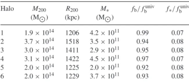
Table 1. Properties of the six simulated clusters studied in this work. The stellar mass is measured within a 30 kpc spherical aperture. The baryon and stellar fractions are measured withinR200and are given
in units of the universal baryon fraction,funiv
b =b/m=0.157.
Halo M200 R200 M∗ fb/fbuniv f∗/fbuniv
(M) (kpc) (M)
1 1.9×10¹⁴ 1206 4.2×10¹¹ 0.99 0.07
2 3.7×10¹⁴ 1518 3.5×10¹¹ 0.94 0.08
3 3.0×10¹⁴ 1411 2.9×10¹¹ 0.95 0.08
4 3.1×10¹⁴ 1422 4.5×10¹¹ 0.97 0.07
5 2.0×10¹⁴ 1225 2.0×10¹¹ 0.92 0.08
6 2.0×10¹⁴ 1229 3.7×10¹¹ 0.93 0.08
Figure 1. Surface brightness map of Cluster 1, using the SDSSugrfilter system. The map is 500 kpc on a side and has resolution of 1 kpc. The central galaxy is easily visible and appears slightly elongated in projection. Satellite galaxies are also visible and cluster around the BCG.
results of this study where we focus on the very centres of the haloes (r20 kpc) where the mass of gas is very small (see Fig.2).
The main properties of our rich cluster sample are listed in Ta-ble1. As shown by Schaye et al. (2015), the galaxy stellar masses are in good agreement with abundance matching relations (Moster, Naab & White2013). At the same time, the overall gas fractions withinR200are close to the cosmic mean,fbuniv=b/m, as
ob-served (Vikhlinin et al.2006): the AGN feedback model has suc-ceeded in suppressing star formation in the BCG without removing excessive amounts of gas from the haloes.
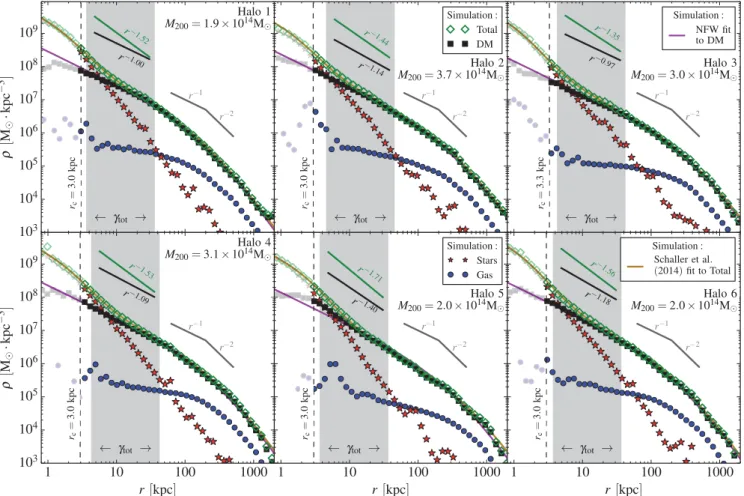
Figure 2. Radial density profiles of the six simulated clusters studied in this paper (see Table1). Green diamonds represent the total mass profile; the black squares, red stars and blue circles represent the DM, stellar and gas components, respectively. The solid magenta and yellow lines are the best-fitting NFW profile to the DM component and the best-fitting (Schaller et al.2015) profile (equation 2) to the total mass distribution. The vertical dashed line in each panel shows the convergence radius,rc, beyond which the density profile has converged to within 20 per cent; data points within this radius are shown by fainter
symbols. The grey shaded regions show the radial range over which the logarithmic slopes,γtotandβDM, of the total and DM profiles are measured. The
values of the slopes are given above the simulation points. The DM haloes are very well fitted by NFW profiles and the total mass profiles only deviate from NFW in the central parts (r10 kpc), where the stellar component dominates. Note the similarities in the shapes of these six haloes and the relatively small variations that occur mostly in the very central regions.
3.1 The mass density profiles of simulated haloes
To study the density profiles of theEAGLEclusters, we bin the parti-cles in logarithmically spaced radial bins centred on the minimum of the gravitational potential. We measure the DM, gas and stellar components separately and then sum all contributions to obtain the total mass profile. The result is shown in Fig.2, where the six panels correspond to the six clusters of Table1. In each panel, the green diamonds, black squares, red stars and blue circles represent the total mass, DM, stellar component and gas, respectively. The mass of each halo is indicated at the top of each panel. The dashed verti-cal lines show the radius,rc, above which the profile is considered
to have converged within 20 per cent (Power et al.2003; Schaller et al.2015). This is a conservative estimate of the convergence ra-dius (∼3.1 kpc) and it is much larger than the Plummer-equivalent softening length ( =0.7 kpc) often used as a rough estimate of the radius beyond which numerical effects become unimportant. Data points within this ‘convergence radius’ but at radiir> are shown using fainter symbols.
The DM dominates the density profiles atr8 kpc. At smaller radii, the stellar component dominates and exceeds the DM density by up to an order of magnitude at the centre. The stellar density
profiles are approximatively constant power laws,r−α, withα≈ −3 down to the very centre of the galaxy. The simulation does not resolve the centre of the BCG and the slopes measured there are probably affected by the force softening (0.7 kpc atz=0) used in theN-body solver. The peaks in the stellar components at large radii are caused by satellites orbiting in the halo. The gas is subdominant at all radii, in particular in the central regions where the stellar densities are almost three orders of magnitude higher. The gas only dominates the baryon content at radiir50 kpc. At radii larger than∼300 kpc, the gas profile has the same shape as the DM profile. The DM itself has the characteristic NFW shape, whose asymptotic behaviour is a power-law of slope−1 at the centre and a power law of slope−3 in the outer parts.
3.2 Fitting models to the simulated haloes
The density profiles of relaxed DM haloes inN-body simulations are well fitted by the near-universal NFW profile which has the form:
ρ(r)
ρcr
= δc
(r/rs) (1+r/rs)2
Table 2. Parameters of the best-fitting NFW profiles (equa-tion 1) to theDMcomponent of our haloes.
Halo M200 R200 rs c200 δc
(M) (kpc) (kpc)
1 1.9×10¹⁴ 1206 199.2 6.1 1.1×10⁴
2 3.7×10¹⁴ 1518 350.8 4.3 5.3×10³
3 3.0×10¹⁴ 1411 452.0 3.1 2.5×10³
4 3.1×10¹⁴ 1422 305.1 4.7 5.9×10³
5 2.0×10¹⁴ 1225 331.1 3.7 3.3×10³ 6 2.0×10¹⁴ 1229 245.9 5.0 7.2×10³
(Navarro et al.1996b,1997), whereδc is a characteristic
ampli-tude andrs, a scalelength that is often expressed in terms of the
concentration,c200=R200/rs. Bothδcandc200correlate with halo
mass,M200, so the NFW profile is fully specified by the halo mass.
In our simulations, the cold gas and stars, which contribute only a small fraction of the total mass, are concentrated towards the cen-tre, while the hot gas beyond the central regions closely follows the DM profile. Thus, even in the presence of baryons, theDM still closely follows an NFW profile. In the case of haloes of mass
M200∼1012-1013M, the profile is slightly modified in the centre
by a modest contraction due to the presence of stars (Duffy et al. 2010; Di Cintio et al.2014; Schaller et al.2015).
Baryon contraction is less important in haloes of massM200∼
1014M
which are well fit by an NFW profile, as can be seen in Fig.2, where the solid magenta line shows the best-fitting NFW profile. The fit was performed using all radial bins from the reso-lution limit,rc∼3 kpc, to the virial radius,Rvir∼2Mpc. We have
checked that the best-fitting parameter values are largely insensitive to the exact radial range used, provided that both theρ(r)→r−1
andρ(r)→r−3regimes of the profile are well sampled. In all but
one case, the magenta line closely tracks the DM profile plotted as black squares. The exception is halo 5 (bottom row, middle panel) which shows a slight deviation from the NFW form in the radial range 3−7 kpc, where some contraction is seen, possibly as a result of the recent accretion of a large substructure. The best-fitting NFW parameters are listed in Table2. The mean and scatter in concen-tration (nearly a factor of 2) of our haloes are consistent with the results obtained for relaxed haloes in the Millennium simulation by Neto et al. (2007), who found a concentration,c200=4.51−+00..7162, for
haloes of massM200=1014M.
While the DM is well described by an NFW profile, thetotal matterprofile in our haloes is not. In our study of the entire halo population in theEAGLE simulation, we introduced the following
fitting formula for the total matter (Schaller et al.2015):
ρ(r)
ρcr
= δc
r/rs 1+r/rs
2+
δi
(r/ri)
1+(r/ri)2
. (2)
The first term has the NFW form and describes the overall shape of the profile; the second term is a correction that reproduces the stellar cusps (ρ∗∝r−3), together with any DM contraction due to the
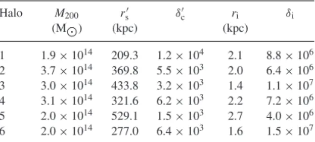
presence of baryons. The dark yellow solid lines in the six panels of Fig.2show the best-fitting profiles of this kind to each halo which, as may be seen from the figure, represent the data well over the entire resolved radial range. The best-fitting parameter values are listed in Table3.
Table 3. Parameters of the best-fitting profiles of the form of equation (2) (Schaller et al.2015) to thetotalmatter distribution in our halo sample.
Halo M200 rs δc ri δi
(M) (kpc) (kpc)
1 1.9×10¹⁴ 209.3 1.2×10⁴ 2.1 8.8×10⁶
2 3.7×10¹⁴ 369.8 5.5×10³ 2.0 6.4×10⁶
3 3.0×10¹⁴ 433.8 3.2×10³ 1.4 1.1×10⁷
4 3.1×10¹⁴ 321.6 6.2×10³ 2.2 7.2×10⁶ 5 2.0×10¹⁴ 529.1 1.5×10³ 2.7 4.0×10⁶ 6 2.0×10¹⁴ 277.0 6.4×10³ 1.6 1.5×10⁷
4 T H E I N N E R D E N S I T Y P R O F I L E
A testable prediction from simulations evolving only DM of the
CDM model is that the average slope of the inner mass profile (rrs) should tend to the NFW value of−1. Steeper profiles might
be explained by baryon effects causing some contraction. Signifi-cantly shallower profiles in massive haloes, on the other hand, would be more difficult to explain. Explosive baryon effects could lower the inner DM density, and even induce cores, but only in dwarf galaxies (Navarro et al.1996a; Read & Gilmore2005; Pontzen & Governato 2014). In massive haloes, Martizzi et al. (2012) have argued that AGN feedback could introduce small (∼10 kpc) cores, but it is unclear if this kind of feedback is compatible with the observed stellar masses of BCGs and the baryon fractions of clus-ters. Shallower inner profiles could also be generated if the DM is self-interacting (Vogelsberger et al.2012; Rocha et al.2013).
4.1 Total mass profiles: simulation results
A quantity that can be derived from observational data in selected samples of rich clusters is theaverage logarithmic slopeof the inner density profile of the total mass, that is DM and baryons (e.g. Sand et al.2004; Newman et al.2013a):
γtot≡ −
d logρtot(r)
d logr
r∈[0.003R200,0.03R200]
, (3)
where the average is over the radial range [0.003R200, 0.03R200]. It
is important to recognize that the radial range typically probed by the data isnotthe asymptotic regime,r→0, where the NFW profile tends toρ(r)∝r−1. Instead, in the region probed by observations,
the NFW formula (equation 1) predicts values of the inner slope significantly steeper than−1 (i.e.γtot>1):
γtot=1+log10
(1+0.03c200)2
(1+0.003c200)2
, (4)
which, for the expected range of cluster concentrations (c200∈[3,
5]), givesγtot≈1.1.
The radial range over whichγtotis typically measured in
obser-vational studies is shown for our clusters as a grey shaded region in each panel of Fig.2. The values of the slope predicted by our simulations in this range are shown above the data points. Values ofγtotfor our halo sample are plotted as a function of halo mass in
Figure 3. The logarithmic slope of the inner density profile of the total mass distribution,γtot, as a function of halo mass,M200. The dashed line shows the
average slope of the NFW profile over the range in whichγtotis defined.
The large green diamonds represent the sixEAGLEhaloes in our sample and
the small green diamonds the smaller massEAGLEhaloes. The grey symbols
with error bars are the slopes measured by Koopmans et al. (2009) for 58 early-type galaxies in the SLACS survey (square), the slope inferred by Agnello et al. (2014) from globular clusters orbits in M87 (triangle) and the slopes measured by Newman et al. (2013a) for seven massive clusters (circles). As a guide, the grey dash–dotted lines demarcate slopes that may be construed as ‘core-like’ and ‘cuspy’. The lower massEAGLE clusters are cuspier than an NFW halo because of the contribution of the stellar component which, however, becomes increasingly less important for larger mass haloes. The Newman et al. (2013a) data lie along the extrapolation of the trend seen in theEAGLEclusters.
considered to be ‘cuspy’ (γtot>1.5) or ‘core-like’ (γtot<0.5). The
exact position of these lines is, of course, arbitrary.
The high-mass tail of the cluster population is not represented in the limited volume of theEAGLEsimulation. However, the general
behaviour of massive clusters can be readily inferred from the trends seen for smaller haloes. A halo of massM200≈2×10¹⁵Mhas
R200≈2 Mpc and thusγtotis centred (logarithmically) aroundr =
20 kpc. In this region the profile is dominated by DM, even in the case of large, extended galaxies. Thus, γtotis unaffected by
the BCG and directly reflects the slope of the DM profile which Schaller et al. (2015) showed has a slope close to or slightly steeper than the NFW value, as given by equation 4. Thus, for haloes ofM200≈2×10¹⁵Mwe expectγtot≈1.1. This conclusion is
consistent with the collisionless model of Laporte & White (2014) who also find slopes close to the NFW value forM200∼1015M
clusters.
Based on this argument we can construct a simple model, consis-tent with the results for low-mass haloes, to extrapolate the slopes measured for the EAGLE clusters into the mass range appropriate to rich clusters. This model is designed to capture the general be-haviour ofγtoton mass scales larger thanM200≈2×10¹³M. It
assumes that the total matter profile is made up of an NFW DM halo plus a stellar component which, in order to be consistent with rele-vant observational analyses, we take to be a ‘dual pseudo isothermal elliptical mass distribution’ (dPIE; El´ıasd´ottir et al.2007). The value of the halo mass determines the concentration of the halo and we infer the stellar mass of the central galaxy from abundance matching (e.g. Moster et al.2013). For the dPIE profile, we adopt the mean scale radius and core radius of the best-fitting profiles for our BCGs and keep them fixed while varying the normalization to match the stellar mass of interest. (We verified that varying the values of the parameters of this model does not affect our results.) In this way
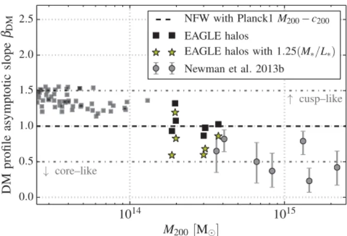
Figure 4. The asymptotic logarithmic slope of the inner DM density profile, βDM, as a function of halo mass,M200. The dashed line shows the NFW value
of−1. The large black squares show the values measured for the six massive clusters in ourEAGLEsample and the small black squares those measured
for smallerEAGLEclusters. The yellow stars show the slopes that would be
inferred for our sample if the stellar mass-to-light ratio is overestimated by 25 per cent (see Section 5.3 for details). The grey circles with error bars are the values inferred by Newman et al. (2013b). As in Fig.3, the grey dash–dotted lines demarcate slopes that may be construed as ‘core-like’ and ‘cuspy’.
we construct the total mass profile and measure its slope, which we show as the green band in Fig.3. The slopes of the total mass profiles of the largestEAGLEclusters plotted in Fig.2are slightly
steeper than the NFW value over the radial range over whichγtot
is defined. This mostly reflects the contribution of stars to the inner matter density. By contrast, the values inferred for more massive clusters are closer to the NFW value.
We now turn to the slope of the DM profiles. Unlike the total mass profile, the DM profile cannot be measured directly from ob-servations, but must instead be inferred through detailed modelling, which requires a number of assumptions. The DM profile in the sim-ulations can, of course, be directly measured and the simsim-ulations can be used to test the consistency of the assumptions required in the modelling of the observational data.
The average slope of the DM density profile over the same radial range used to defineγtot([0.003R200, 0.03R200]) for our sample of
simulated clusters is indicated by the black line in the grey shaded regions in Fig.2. Some observational analyses attempt to constrain the asymptotic slope,βDM, of a generalized NFW profile (gNFW):
ρgNFW(r)
ρcr
= δc
(r/rs)βDM(1+r/rs)3−βDM
. (5)
This profile is often used to quantify deviations from the NFW form to which it reduces forβDM=1 (equation 1). We fit this profile to
the DM of our simulated haloes and plot the resulting values ofβDM
as a function of halo mass,M200, in Fig.4, which is the DM analogue
of Fig.3. As may be seen, theEAGLEclusters (black squares) have
inner slopes consistent with the NFW expectation (equation 4). As was the case for the total matter profile, the inner DM profile slopes also show significant scatter, withβDMvarying by as much as∼0.4
for haloes of similar mass.
4.2 Total mass profiles: overview of recent observational data
to probe the central mass distributions: strong lensing and modelling of the orbits of globular clusters (GC) or BCG stars. The former relies on a chance alignment of the cluster with a background galaxy and is, by nature, rare since only a few galaxy clusters present strong lensing arcs at the radii of interest. Similarly, the use of GC orbits as tracers of the potential is limited to clusters that are close enough for the GCs to be unambiguously detected. Stellar velocity dispersion measurements of the central galaxy can also be used to constrain the mass near the centre of the halo but high-resolution spectroscopy is required. We will now compare our simulated cluster slopes to recent observational data. Although there is a wealth of data available for profiles at large radii, we focus exclusively on the inner regions which are the most sensitive to the nature of the DM. The grey square with error bars at the low mass end of Fig.3 shows the average slope measured for 58 early-type galaxies in the SLACS survey by Koopmans et al. (2009) using a combination of strong lensing and stellar velocity dispersion measurements. Our simulation agrees perfectly with this data point. At the more massive end, Newman et al. (2013a) derived total mass profiles, ρtot(r),
from projected mass profiles, which they estimated using strong and weak lensing data, together with the surface brightness and resolved stellar kinematics of the BCGs in a sample of seven clusters. The grey circles with error bars in Fig.3show their results. Five of these clusters have higher masses than the largest clusters in the relatively smallEAGLEsimulation volume, but the two lightest ones fall in the
region represented in our simulation. Their values ofγtotagree very
well with those measured directly in our simulated clusters while the values for the more massive five lie in the region predicted by the simple model used to extrapolate theEAGLEresults described in
Section 4.1.
An independent measurement of the total inner density profile which does not rely on lensing data was carried out by Agnello et al. (2014) using the orbits of GCs in the halo of M87. The slope,γtot, inferred from their best-fitting broken power-law model
is shown as a triangle with error bar In Fig.3, this data point also agrees extremely well with the results for theEAGLEclusters.
We conclude that the inner density profiles of the totalmass distribution in theEAGLEclusters are in good agreement with the
best current data Koopmans et al. (2009), Newman et al. (2013a) and Agnello et al. (2014). In both simulated and observed clusters, the inner profile slopes exhibit considerable scatter reflecting the variety of factors that affect the density structure, such as halo assembly history, shape and substructure distribution, BCG star formation and merger history, etc.
4.3 DM density profiles
The situation is more complicated for the density profile of the DM since this is not directly accessible to observations. Instead, this profile must be inferred from a model to disentangle the contribu-tions of the dark and visible components from the measured total mass profile. Wide radial coverage is needed fully to sample the two components and effect the decomposition. Strong lensing data sel-dom sample the range,r10 kpc, where the influence of baryons starts to play a role and so lensing data need to be supplemented by, for example, kinematical data for the stars of the BCG. Such data exist for only a handful of clusters (e.g. Sand et al.2004; Newman et al.2013a). The study by Newman et al. (2013a) is particularly in-teresting by virtue of the quality of the data and the comprehensive analysis performed. In the remainder of this paper, we will therefore focus on the comparison with these data.
The model assumed by Newman et al. (2013a) is a gNFW profile for the DM and a dPIE profile for the galaxy. The authors esti-mated the parameters values that minimize the difference between the model and the inferred lensing mass, the measured profiles of stellar velocity dispersion,σl.o.s., and surface brightness,S. In
addi-tion to the parameters describing the DM profile, the minimizaaddi-tion procedure also constrains the stellar mass-to-light ratio,ϒ∗. This is an important parameter since, at a given radius, it is degenerate with the dark matter mass: one can always trade DM for unseen stellar mass at that radius,
ρDM(r)=ρtot(r)−ϒ∗×S(r). (6)
This degeneracy can be broken by measuring the total density and surface brightness as a function of projected radius,R, and assuming that the stellar mass-to-light ratio is constant.
The values ofβDM(equation 5) inferred by Newman et al. (2013b)
for their sample of clusters are shown as grey circles in Fig.4. The error bars indicate the 16th and 84th percentiles of the posterior distribution ofβDMreturned by their model (not including
system-atics). These lie well below the values for theEAGLEclusters (black
squares) and are clearly inconsistent with them given the quoted errors. From our earlier discussion it seems unlikely that the dis-crepancy can be due to the slightly smaller masses of theEAGLE
clusters compared to those in the observed sample, since theEAGLE
clusters have DM inner slopes that are either close to or slightly steeper (due to contraction) than the NFW value. Thus, we con-clude that profile slopes as shallow as those inferred by Newman et al. (2013b) are not present inCDM simulations with the baryon physics modelled inEAGLE. This conclusion is surprising since the
totalmass profiles of the real and simulated clusters agree remark-ably well. We will now discuss possible reasons for this apparent discrepancy.
5 D I S C U S S I O N
We saw in the preceding section that the inner slopes of the density profiles of the DM haloes in theEAGLEclusters differ from the
pro-files inferred by Newman et al. (2013b) for their sample of seven clusters. There are several possible explanations for the discrepancy. One is that the simulations do not model the correct physics. This would be the case if the DM does not consist of cold collisionless particles but of particles that undergo self-interactions (e.g. Spergel & Steinhardt2000; Vogelsberger et al.2012; Rocha et al.2013). Cluster simulations would be required to determine whether the slopes found by Newman et al. (2013a) can be explained for rea-sonable values of the self-interaction cross-section and a rearea-sonable model for the baryonic physics.
The disagreement between the inner DM profiles of theEAGLE
clusters and of the clusters in the Newman et al. (2013b) sample could also be due to a mismatch between the directly observable quantities,σl.o.s.(R) andS(R), and the corresponding quantities for
theEAGLEclusters, or to systematic effects either in the selection of
the observational sample or in the method used to inferred the inner DM slopes. We will now discuss these possibilities.
The most direct way to carry out the comparison would be to replicate the analysis of Newman et al. (2013a) on our simulated clusters. Unfortunately, the exact model and fitting pipeline used by them is not available to us and, as we will see below, the results are very sensitive to small changes in the assumption of the analysis pipeline. We therefore restrict our comparison to directly observable quantities and discuss how some of the assumptions made could impact the inferred values ofβDM.
5.1 Surface brightness profiles
Stars are the dominant contributors to the density in the central regions of theEAGLE clusters and probably also in the real data.
Clearly, if the surface brightness of the simulated clusters differed significantly from the observations, subtraction of this component could lead to different results for the slope of the DM profile in the two cases.
As discussed in Section 2.2, the luminosity of each stellar particle in the simulations is obtained from aBC03population synthesis model assuming the Chabrier (2003) IMF. To compare our haloes with observations, we derive magnitudes in the four HSTfilters (F606W, F625W, F702W and F850LP) used by Newman et al. (2013a). We placed our clusters atz=0.25, the mean redshift of that sample, by redshifting the spectra before applying theHSTfilters2
and dimming the luminosities by a factor (1 +z)−4. To account
for the somewhat smaller masses of theEAGLEclusters compared to
those in the sample of Newman et al. (2013a) (whose mean mass is
M200=1.03×10¹⁵M) we scaled up their surface brightnesses
by a modest factor, (M200/1.03×1015M)1/6, derived assuming
that the luminosityL∝M2001/2and that the stellar density remains
constant in the narrow range or relevant halo masses.3We then chose
10 000 random lines of sight through each cluster and projected the particles along those axes on to the plane of the (virtual) sky. Finally, we binned the particles radially from the centre of the potential to derive the stellar surface brightness.
The surface brightness profiles of our sixEAGLEclusters are plot-ted in Fig.5. The solid lines show the mean profiles averaged over 10 000 lines of sight in the four differentHSTfilters and the shaded regions the 1σscatter around these values. The black symbols corre-spond to the measurements taken from Newman et al. (2013a) with physical radii derived from their angular sizes and redshift mea-surements. Although theEAGLEclusters have a slightly smaller total
mass, the surface brightness of their central galaxies are in quite good agreement with those of the Newman et al. (2013a) sample: the shapes of the profiles are somewhat different, with our clusters having a slightly shallower inner slope than the observed clusters.
A striking feature of Fig.5is the small scatter in the simula-tions for the different lines of sight. Near the centre the scatter is dominated by the presence of foreground satellites rather than by the orientation of the BCG. Another interesting feature is the large
2Effectively applying a reverseK-correction.
3Note that this is a more conservative rescaling factor than simply assuming
L∝M200.
object-to-object variation, both in the simulations, where the cen-tral luminosities vary by around 0.8 mag, and in the observations, where the variation is even larger, almost 2 mag, with no apparent correlation with halo mass. Our simulated haloes lie well within the observational scatter but themselves show somewhat smaller scatter. At large radii, five out of our six clusters appear to be slightly more luminous than the real clusters. However, this is the region where the observational data terminate and where background subtraction becomes significant.
We conclude that the surface brightness profiles of theEAGLE
clus-ters are sufficiently similar to those of the Newman et al. (2013b) sample that differences in the starlight distribution cannot be the rea-son for the discrepancy between the DM profiles in the simulations and those inferred from the data.
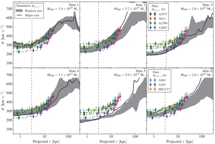
5.2 Velocity dispersion profiles
The line-of-sight stellar velocity dispersion,σl.o.s., of our six haloes
as a function of projected radius is shown in Fig.6. Since the
EAGLEclusters are less massive than the clusters in the sample of
Newman et al. (2013a), in order to facilitate a comparison, the velocity dispersions of the simulated clusters have been rescaled, as before, to the mean mass of the Newman et al. (2013a) sample by multiplying the velocity dispersions by the corresponding factor (M200/1.03×1015M)1/6.
The measuredσl.o.s.is quite sensitive to the shape of the galaxy
and the viewing angle. The axial ratios, of the six EAGLE BCGs
(computed from the principal axes of the inertia tensor of the star particlesa>b>c) are illustrated in Fig.7where the projection along the minor axis is shown at the top of each panel and the projection along the major axis at the bottom. Four of the sixEAGLE
clusters (1, 2, 5 and 6) are clearly prolate and the remaining two are close to spherical. We viewed the BCGs from 10 000 random directions placing an imaginary slit at a random angle on the plane of the sky centred on the halo potential minimum and measured the velocity dispersion of the stars as a function of projected radius, subtracting any bulk rotation.
As expected, the line-of-sight velocity dispersions increase with radius. In the inner regions (r10 kpc) gravity is dominated by the stars. The 1σ scatter from the different viewing angles, shown as a grey shaded region in Fig.6, is rather large at all radii for all objects, of the order of 10 per cent or more for all but two of the haloes. The black solid line showsσl.o.s. for a line of sight chosen along the
major axis of each BCG. In three of our six clusters (haloes 2, 5 and 6), the velocity dispersion along this particular line of sight is biased high and, in two cases, it falls outside the 1σscatter. As can be seen on Fig.7, these are the three most prolate haloes in our sample. A bias in the line-of-sight velocity dispersion is expected since orbits in prolate haloes have larger velocities along the direction of elongation. These objects would nevertheless appear spherical on the sky when viewed in this direction since the axis ratiosb/care close to unity. The three most spherical haloes do not exhibit any particular bias when viewed along their major axis, as expected.
The line-of-sight velocity dispersion profiles of the seven clusters studied by Newman et al. (2013a) are shown as dashed colour lines with error bars in each panel of Fig.6. The six rescaledEAGLEclusters
have dispersions that fall within the scatter of the observational data. Thus, unless there is a strong orientation bias for the BCGs in the cluster sample of Newman et al. (2013a), a mismatch in velocity dispersion profile cannot be the cause of the difference between the slopes of the DM haloes in theEAGLEclusters and those inferred by
Figure 5. Surface brightness profiles of the sixEAGLEclusters in our sample (placed atz=0.25) in the fourHSTfilters (from top to bottom:F850LP, F702W,F625WandF606W) used by Newman et al. (2013a) in AB magnitudes per arcsec−2. The solid lines show the mean profile scaled by the factor, (M200/1.03×1015M)1/6, averaged over 10 000 random lines of sight. The shaded regions show the 1σscatter for the reddest and bluest filters. (The other
filters have similar scatter.) The black symbols show the measured surface brightness profiles of the seven clusters observed by Newman et al. (2013a) whose redshifts are given in the legend together with the filter used. The clusters in the simulations have surface brightness profiles in reasonable agreement with those observed.
Since the projected mass density of a prolate halo is also largest along its major axis, there is a potential and well-understood se-lection bias in samples of clusters selected for lensing studies. If the BCGs in the sample of Newman et al. (2013a) were prolate and preferentially viewed along their major axes, then, as shown in Fig.6, the observed line-of-sight velocity dispersions would be bi-ased high. This would lead to an overestimate of the mass enclosed within the radius sampled by the velocity dispersion data. In the ab-sence of other information, it would not be possible to separate the relative contributions to this estimate from stars and DM. However, the available lensing data constrains the total mass (and, in the case of radial arcs, also the slope of the profile) in the central regions of the cluster. This, together with the inferred stellar profile, restricts the fits to the combined data and this could lead to an underestimate of the DM mass near the centre of the clusters.
Such an effect could explain the difference between the slopes of the DM profiles inferred by Newman et al. (2013a) and those measured for theEAGLEclusters. However, Newman et al. (2013a)
argue that their sample does not suffer from such a bias since the distribution of ellipticities in it is consistent with that of the BCG population as a whole. In the case of A383, for which the X-ray data indicate is elongated along the line of sight, they explicitly use a non-spherical model.
5.3 Mass-to-light ratio
As mentioned in Section 4.2, the stellar mass density at a given radius is degenerate with the DM mass density at that radius (equa-tion 6). In the simula(equa-tions we know the stellar mass and so we can subtract it exactly from the total mass. The resulting value of the inner DM halo slope was shown in Fig.4. By contrast, in the obser-vational sample the stellar mass must be derived from an estimate of the stellar mass-to-light ratio,ϒ∗.
Figure 6. Stellar velocity dispersion along the line of sight as a function of projected radius for the sixEAGLEclusters listed in Table1. The dispersions have
been rescaled by a factor (M200/1.03×1015M)1/6to correct for the slightly lower masses of these clusters compared to the mean of the observational
sample of Newman et al. (2013a). The grey shaded region is the 1σscatter obtained when looking at the haloes from 10 000 random lines of sight. The black solid line is the profile as seen from a line of sight oriented along the galaxy’s major axis. The vertical dashed line on each panel shows the 3D convergence radius,rc. The coloured dashed lines with error bars are the measurements for the seven clusters observed by Newman et al. (2013a). In three of the sixEAGLE
haloes the velocity dispersion profile measured along the major axis is biased high.
In Fig.4, we show the effect of overestimatingϒ∗by a much smaller factor of only 25 per cent. The inferred slopes, shown by yellow stars, are significantly shallower than the true slopes and have more scatter. Such a relatively small systematic error would be sufficient to bring the inferred slopes in the simulations into agreement with the estimates of Newman et al. (2013b).
The estimate of ϒ∗ in the model of Newman et al. (2013b) requires the measurement of the line-of-sight velocity dispersion profile,σl.o.s., of the BCG, as a function of projected separation,R.
In dynamical equilibrium,σl.o.s.is given by the Jeans equation (e.g.
Binney & Tremaine1987; Cappellari2008):
σ2 l.o.s.(R)=
2G
∗(R) ∞
R
F(r, R, β)ρ∗(r)Mtot(r)
r2−2β dr, (7)
whereρ∗(r) is the 3D density of tracers (the stars) whose surface density is∗(R);Mtot(r) is the total enclosed mass;β=1−σθ2/σr2
is the velocity anisotropy parameter, here assumed to be indepen-dent of radius, with σrandσθ the radial and tangential velocity
dispersions, respectively,4and
F(r, R, β)= R
1−2β
2 βB
R2
r2;β+
1 2,
1 2
−B
R2
r2;β−
1 2,
1 2
+ √
π(3−2β)(β− 1 2)
2(β)
,
where(x) is the Gamma function andB(z;a,b) is the incomplete Beta function. In the limit whereβ→0,F(r, R, β) reduces to
lim
β→0F(r, R, β)=
r2−R2.
In the more general case whereβis a function ofr, the problem of reconstructing the mass distribution becomes more complex. Solutions for specific forms ofβ(r) have been derived by Mamon & Bou´e (2010).
In the Jeans equation, the velocity anisotropy parameter and the mass are degenerate. In their analysis Newman et al. (2013a) as-sumed β = 0 i.e. isotropic orbits. This assumption is a source of a potentially significant systematic error which Newman et al.
4With this definition,β=0, 1 and−∞correspond to isotropic, radially
Figure 7. The projection of the central stellar component of the sixEAGLE
clusters along the minor axis (top ellipse in each panel) and major axis (bottom ellipse). The axes ratios are given next to each ellipse. Four of the galaxies are clearly prolate and the remaining two are slightly oblate. Prolate galaxies have velocity dispersions that are biased high (Fig.6) when observed along their major axis.
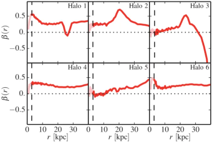
(2013a) investigated. They found that if the orbits were mildly ra-dially biased with a constant value ofβ= +0.2, thenϒ∗would be overestimated by 30 per cent. In our simulations we can calcu-lateβdirectly for the stars in the model BCGs. The variation ofβ with radius is shown in Fig.8. We find that, in general,βvaries with radius over the range where Newman et al. (2013a) obtained kinematical data. In two of our clusters,βis close to zero over this range, but in the other four,βbecomes increasingly positive with radius, with a mean value of∼0.2–0.3. Complex features, which cannot be described by a simple linear form forβ(r) are also present, precluding the reconstruction ofM(r) from an assumed functional form forβ(r). It is also worth mentioning that the profile ofβ(r) is uncorrelated with the shape of the BCGs: of the two cases with nearly isotropic orbits (haloes 3 and 5), one is nearly spherical and the other very elongated (see Fig.7).
In order to test the assumption of anisotropy, we inverted equa-tion (7) numerically. Extractingσl.o.s.(R), ∗(R) and ρ∗(r) from the simulated clusters we reconstructedMtot(r) assumingβ = 0
and compared the result to the actual value. We found that for this assumption the reconstruction overestimates the value ofMtotby
factors ranging from 10 to over 100 per cent. Repeating this analy-sis, this time assumingβ=0.2, led to errors of comparable size for the four haloes that display an anisotropy profile differing signifi-cantly fromβ(r)=0.2 (see Fig.8). Thus, for most of our clusters, the analysis of Newman et al. (2013a) would have overestimated the stellar mass-to-light ratio by more than the 25 per cent which, according to Fig.4, would reconcile their results with our simula-tions. This test, however, does not take into account constraints on thetotalmass profile from lensing data at large radii, which could exaggerate the dependence of the inferred value ofMtot near the
centre on the assumed value ofβ.
In real clusters, additional uncertainties are introduced by factors such as an assumed form for the 3D stellar mass density profile,
ρ∗(r), and an assumption for the value of the stellar mass-to-light ratio, ϒ∗. This is mitigated by constraints on Mtot provided by
lensing data although, in general, the lensing and kinematical data do not overlap sufficiently to separate the contributions from the stellar mass and the dark mass. In the model of Newman et al. (2013a),
ϒ∗is coupled to other parameters such as the slope of the total mass profile, so that the effect on the quantity of interest,βDM, is
Figure 8. Stellar anisotropy profileβ(r) as a function radius for the sixEAGLE
clusters over the radial range relevant to the stellar kinematics analysis. The vertical dashed line on each panel shows the 3D convergence radius,rc
and the profiles at lower radii are shown using shaded lines. Two BCGs are consistent withβ=0 but would be better fit with a non-constantβ. Ignoring complex features, the other four clusters present more radially biased orbits withβ(r)≈0.25. A single profile shape forβ(r) cannot be used to characterize all six of our BCGs.
difficult to anticipate without re-running their pipeline for different assumptions for the velocity anisotropy. For example, Newman et al. (2013b) tried a solution for the case of constant anisotropy,β=0.2, and found an increase inβDM of about 0.13, which would bring
their data closer to our simulations. What we can say with certainty is that the kinematical model assumed by Newman et al. (2013a) is not consistent with theEAGLEBCGs, offering a possible explanation
for the discrepancy in the DM density slopes.
Constraining the anisotropy,β, in cases in which, as in our simu-lated clusters, it varies with radius is not straightforward. Yet, this is what is required in order to lift the degeneracy between anisotropy and mass which lies behind the degeneracy betweenϒ∗ and the DM profile slope. The use of Integral Field Spectroscopy may help constrain this quantity in future studies.
6 S U M M A RY A N D C O N C L U S I O N S
We have studied the density profiles of the six most massive clusters in the largestEAGLEsimulation (Schaye et al.2015). TheEAGLE simu-lation was calibrated to provide a good match to the observed stellar mass function and galaxy sizes in the local universe, suggesting that it gives a realistic representation of the local galaxy population. Due to the relatively small volume of the simulation (1003Mpc3), the
clusters selected for this study tend to be somewhat less massive (meanM200=2.6×10¹⁴M) than the seven clusters studied by
Newman et al. (2013a) (meanM200=1×10¹⁵M) to which we
compare our results in particular detail, although the two light-est clusters in the observational sample have similar masses to the three most massiveEAGLEclusters. For these clusters Newman et al.
(2013a) have obtained strong and weak lensing as well as stellar kinematical data for the BCGs.
The total mass density profile of theEAGLEclusters is dominated
survey, and with the slope inferred by Agnello et al. (2014) from the kinematics of GCs around M87.
The DM density profile of theEAGLEclusters is very well
de-scribed by the NFW profile over the entire resolved radial range,
r=3-2000 kpc. By contrast, Newman et al. (2013b), after subtract-ing the contribution of the stars, inferred significantly shallower DM slopes for their clusters in the inner regions, in contradiction with our own results. This discrepancy is puzzling because, in addition to the total mass density profiles, the surface brightness and line-of-sight velocity dispersion profiles of theEAGLEclusters agree quite
well with those of the Newman et al. (2013a) clusters.
We have considered possible explanations for the discrepancy between the inner DM density profiles of theEAGLEclusters and
those inferred by Newman et al. (2013b). A possible interpretation is that the simulations lack the correct physics, either because the DM is not collisionless (e.g. Spergel & Steinhardt2000; Vogelsberger et al.2012; Rocha et al.2013) or because extreme baryon processes not represented in our simulations have destroyed the inner DM cusps (Martizzi et al.2012). Baryon effects associated with AGN in theEAGLEsimulations are not strong enough to produce density
cores; yet the simulation reproduces the exponential cut-off in the stellar mass function remarkably well.
An alternative explanation for the discrepancy is that the uncer-tainties in the determination of the inner DM density slope were underestimated by Newman et al. (2013b). In particular, their anal-ysis relies on an accurate estimate of the stellar mass-to-light ratios of the BCGs. We showed that a systematic overestimation of this ratio by only 25 per cent would reconcile the observational data with our results. An effect of this size could be produced if the measured stellar velocity dispersions were biased high as would be the case if the BCGs (which are all selected to be strong gravitational lenses) were prolate and preferentially viewed along their major axis. How-ever, Newman et al. (2013a,b) have argued that such a selection bias is unlikely in their sample since the distribution of BCG ellipticities appears to be typical of a randomly oriented population.
Another possible source of systematic error in the estimate of the stellar mass-to-light ratio is the assumption made by Newman et al. (2013b) that the stars in the BCG have a uniform and isotropic distribution of orbits. In their paper, they showed that mildly radial orbits would lead to an overestimate of the stellar mass-to-light ratio of 30 per cent, sufficient, in principle, to account for the dis-crepancy with the NFW inner DM slopes of theEAGLEclusters. We
find that just such a situation is present in four of our six clusters which show radially biased orbital distributions which vary with radius in a complicated way. However, in practice, the situation is not straightforward because the mass-to-light ratio in the model of Newman et al. (2013a) is coupled to other parameters and is sensitive to the constraints on the total mass profile from lensing.
We can conclude, however, that systematic errors resulting from the assumptions made in the analysis of Newman et al. (2013b) could potentially be large enough to account for the shallow inner DM profiles that these authors infer for their clusters, in conflict with the cuspy profiles found for theEAGLEclusters. Unfortunately, it is
very difficult, if not impossible, to break the degeneracies inherent in stellar kinematical analyses with existing data. High-resolution integral field spectroscopy of BCGs could prove helpful in future work.
AC K N OW L E D G E M E N T S
We thank Lydia Heck and Peter Draper for their indispensable technical assistance and support. We also thank for Drew Newman
and Tomasso Treu for comments on an early draft of this paper which influenced its final form. RAC is a Royal Society Univer-sity Research Fellow. This work was supported by the Science and Technology Facilities Council (grant number ST/F001166/1); by the Dutch National Computing Facilities Foundation (NCF) for the use of supercomputer facilities, with financial support from the Netherlands Organization for Scientific Research (NWO); the European Research Council under the European Union’s Sev-enth Framework Programme (FP7/2007-2013)/ERC grant agree-ments 278594-GasAroundGalaxies, GA 267291 Cosmiway, GA 238356 Cosmocomp and the Interuniversity Attraction Poles Pro-gramme initiated by the Belgian Science Policy Office ([AP P7/08 CHARM]). It used the DiRAC Data Centric system at Durham University, operated by the Institute for Computational Cosmology on behalf of the STFC DiRAC HPC Facility (www.dirac.ac.uk). This equipment was funded by BIS National E-infrastructure cap-ital grant ST/K00042X/1, STFC capcap-ital grant ST/H008519/1 and STFC DiRAC Operations grant ST/K003267/1 and Durham Uni-versity. DiRAC is part of the National E-Infrastructure. We ac-knowledge PRACE for awarding resources in the Curie machine at TGCC, CEA, Bruy`eres-le-Chˆatel, France.
R E F E R E N C E S
Agnello A., Evans N. W., Romanowsky A. J., Brodie J. P., 2014, MNRAS, 442, 3299
Binney J., Tremaine S., 1987, Galactic Dynamics. Princeton Univ. Press, Princeton, NJ, p. 747
Blumenthal G. R., Faber S. M., Flores R., Primack J. R., 1986, ApJ, 301, 27 Booth C. M., Schaye J., 2009, MNRAS, 398, 53
Bruzual G., Charlot S., 2003, MNRAS, 344, 1000 (BC03) Cappellari M., 2008, MNRAS, 390, 71
Chabrier G., 2003, PASP, 115, 763 Charlot S., Fall S. M., 2000, ApJ, 539, 718 Crain R. A. et al., 2009, MNRAS, 399, 1773 Crain R. A. et al., 2015, MNRAS, 450, 1937 Dalla Vecchia C., Schaye J., 2012, MNRAS, 426, 140
Davis M., Efstathiou G., Frenk C. S., White S. D. M., 1985, ApJ, 292, 371 Di Cintio A., Brook C. B., Dutton A. A., Macci`o A. V., Stinson G. S., Knebe
A., 2014, MNRAS, 441, 2986 Doi M. et al., 2010, AJ, 139, 1628
Dolag K., Borgani S., Murante G., Springel V., 2009, MNRAS, 399, 497 Duffy A. R., Schaye J., Kay S. T., Vecchia C. D., Battye R. A., Booth C. M.,
2010, MNRAS, 105, 2161
Durier F., Dalla Vecchia C., 2012, MNRAS, 419, 465 Dutton A. A., Macci`o A. V., 2014, MNRAS, 441, 3359 El´ıasd´ottir ´A. et al., 2007, preprint (arXiv:0710.5636) Furlong M. et al., 2015, MNRAS, 450, 4486
Gao L., Navarro J. F., Cole S., Frenk C. S., White S. D. M., Springel V., Jenkins A., Neto A. F., 2008, MNRAS, 387, 536
Gao L., Navarro J. F., Frenk C. S., Jenkins A., Springel V., White S. D. M., 2012, MNRAS, 425, 2169
Gnedin O. Y., Kravtsov A. V., Klypin A. A., Nagai D., 2004, ApJ, 616, 16 Gnedin O. Y., Ceverino D., Gnedin N. Y., Klypin A. A., Kravtsov A. V.,
Levine R., Nagai D., Yepes G., 2011, preprint (arXiv:1108.5736) Haardt F., Madau P., 2001, in Neumann D. M., Tran J. T. V., eds, Clusters
of Galaxies and the High Redshift Universe Observed in X-rays. CEA, Savoie, France
Hopkins P. F., 2013, MNRAS, 428, 2840 Jenkins A., 2010, MNRAS, 403, 1859 Jenkins A., 2013, MNRAS, 434, 2094 Koopmans L. V. E. et al., 2009, ApJ, 703, L51
Laporte C. F. P., White S. D. M., 2014, preprint (arXiv:1409.1924) Lupton R., Blanton M. R., Fekete G., Hogg D. W., O’Mullane W., Szalay
Mamon G. A., Bou´e G., 2010, MNRAS, 401, 2433
Martizzi D., Teyssier R., Moore B., Wentz T., 2012, MNRAS, 422, 3081 Moster B. P., Naab T., White S. D. M., 2013, MNRAS, 428, 3121 Navarro J. F., Eke V. R., Frenk C. S., 1996a, MNRAS, 283, L72 Navarro J. F., Frenk C. S., White S. D. M., 1996b, ApJ, 462, 563 Navarro J. F., Frenk C. S., White S. D. M., 1997, ApJ, 490, 493 Navarro J. F. et al., 2004, MNRAS, 349, 1039
Navarro J. F. et al., 2010, MNRAS, 402, 21 Neto A. F. et al., 2007, MNRAS, 381, 1450
Newman A. B., Treu T., Ellis R. S., Sand D. J., Nipoti C., Richard J., Jullo E., 2013a, ApJ, 765, 24
Newman A. B., Treu T., Ellis R. S., Sand D. J., 2013b, ApJ, 765, 25 Okabe N., Smith G. P., Umetsu K., Takada M., Futamase T., 2013, ApJ, 769,
L35
Okamoto T., Shimizu I., Yoshida N., 2014, PASJ, 66, 70 Planck Collaboration XVI, 2014, A&A, 571, A16
Pointecouteau E., Arnaud M., Pratt G. W., 2005, A&A, 435, 1 Pontzen A., Governato F., 2012, MNRAS, 421, 3464 Pontzen A., Governato F., 2014, Nature, 506, 171 Portinari L., Chiosi C., Bressan A., 1998, A&A, 334, 505
Power C., Navarro J. F., Jenkins A., Frenk C. S., White S. D. M., Springel V., Stadel J., Quinn T., 2003, MNRAS, 338, 14
Read J. I., Gilmore G., 2005, MNRAS, 356, 107
Rocha M., Peter A. H. G., Bullock J. S., Kaplinghat M., Garrison-Kimmel S., O˜norbe J., Moustakas L. A., 2013, MNRAS, 430, 81
Rosas-Guevara Y. M. et al., 2013, preprint (arXiv:1312.0598) Sand D. J., Treu T., Smith G. P., Ellis R. S., 2004, ApJ, 604, 88
Scannapieco C. et al., 2012, MNRAS, 423, 1726 Schaller M. et al., 2015, MNRAS, 451, 5765 Schaye J., 2004, ApJ, 609, 667
Schaye J., Dalla Vecchia C., 2008, MNRAS, 383, 1210 Schaye J. et al., 2010, MNRAS, 402, 1536
Schaye J. et al., 2015, MNRAS, 446, 521
Spergel D. N., Steinhardt P. J., 2000, Phys. Rev. Lett., 84, 3760 Springel V., 2005, MNRAS, 364, 1105
Springel V., White S. D. M., Tormen G., Kauffmann G., 2001, MNRAS, 328, 726
Strigari L. E., Frenk C. S., White S. D. M., 2010, MNRAS, 408, 2364 Strigari L. E., Frenk C. S., White S. D. M., 2014, preprint (arXiv:1406.6079) Trayford J. W. et al., 2015, preprint (arXiv:1504.04374)
Tremonti C. A. et al., 2004, ApJ, 613, 898 Umetsu K. et al., 2014, ApJ, 795, 163
Vikhlinin A., Kravtsov A., Forman W., Jones C., Markevitch M., Murray S. S., Van Speybroeck L., 2006, ApJ, 640, 691
Vogelsberger M., Zavala J., Loeb A., 2012, MNRAS, 423, 3740 Vogelsberger M. et al., 2014, Nature, 509, 177
Walker M. G., Penarrubia J., 2011, ApJ, 742, 20
Wiersma R. P. C., Schaye J., Smith B. D., 2009a, MNRAS, 393, 99 Wiersma R. P. C., Schaye J., Theuns T., Dalla Vecchia C., Tornatore L.,
2009b, MNRAS, 399, 574