MULTIPLE INPUT SINGLE OUTPUT CONVERTER WITH MAXIMUM POWER POINT TRACKING FOR RENEWABLE ENERGY APPLICATIONS

MULTIPLE INPUT SINGLE OUTPUT CONVERTER WITH MAXIMUM POWER POINT TRACKING FOR RENEWABLE ENERGY APPLICATIONS

A Thesis presented to

the Faculty of California Polytechnic State University, San Luis Obispo

In Partial Fulfillment of the Requirements for the Degree Master of Science in Electrical Engineering

by Kenneth Nguyen

iii

COMMITTEE MEMBERSHIP

TITLE: Multiple Input Single Output Converter with Maximum Power Point Tracking for Renewable Energy

Applications

AUTHOR: Kenneth Nguyen

DATE SUBMITTED: May 2020

COMMITTEE CHAIR: Taufik, Ph.D.

Professor of Electrical Engineering

COMMITTEE MEMBER: Vladimir Prodanov, Ph.D.

Associate Professor of Electrical Engineering

COMMITTEE MEMBER: Majid Poshtan, Ph.D.

iv ABSTRACT

Multiple Input Single Output Converter with Maximum Power Point Tracking for Renewable Energy Applications

Kenneth Nguyen

v

ACKNOWLEDGMENTS

I would like to thank first and foremost my parents and family for helping me to this point. I appreciate the love and support they have given me. Secondly, I have nothing but gratitude and thanks for Dr. Tafuik, who has guided and assisted me though this Thesis to the best of his ability. Without either parties help, I would not be here today.

Thirdly, I’d to thank my friends and colleagues who’ve both kept my spirits up in finishing this thesis as well as giving me advice or assistance when I needed it. My thesis partner, Kristen, supported me and has been someone to bounce ideas, which I am grateful for. I’m also grateful to my two mentors, Nick and Kevin for always providing me advice and their friendship.

vi

TABLE OF CONTENTS

Page

LIST OF TABLES ….. ... vii

LIST OF FIGURES ... viii

CHAPTER 1. INTRODUCTION ... 1

2. BACKGROUND ... 3

2.1 Renewables ... 3

2.2 Maximum Power Point Tracking (MPPT) ... 6

2.3 Multiple Input Single Output (MISO) ... 8

3. DESIGN REQUIREMENTS ... 10

4. SYSTEM DESIGN AND SIMULATION ... 13

4.1 Component Selection ... 13

4.2 Board Design ... 22

4.3 Simulation Results ... 25

4.4 Software Definition ... 34

5. HARDWARE TESTING AND RESULTS ... 36

5.1 System Construction ... 37

5.2 Test Setup and Results ... 39

6. CONCLUSION ... 51

BIBLIOGRAPHY ... 53

APPENDICES A. Rigol DP-832: Solar Panel Code ... 55

B. Arduino Code ... 59

vii LIST OF TABLES

Table Page

3-1. Summary of Design Requirements ... …...…12

4-1. Relationship between Modulation Voltage, Period, and Duty Cycle... 29

4-2. Simulation Results of the Proposed System at Various Operating Conditions ... 32

5-1. Irradiance Curve Points ... 43

5-2. Test Results with MPPT Stage ... 45

viii LIST OF FIGURES

Figure Page

1-1. Electrification ratio of rural areas in developing countries ...…1

1-2. Functional block diagram of the DC House project ... 2

2-1. IV Solar Panel Characteristics ... 4

2-2. Wind Turbine Block Diagram ... 5

2-3. DC Wind Turbine ... 5

2-4. Wind Turbine Output Power Curve ... 7

2-5. MPPT Power Difference ... 7

3-1. Level 0 block diagram of the proposed system ... 10

3-2. Level 1 block diagram of the proposed system 15 ... 11

4-1. Low Level Block Diagram of a Single Converter ... 13

4-2. Rise/Fall Time of the LTC7004 ... 14

4-3. Standard Bootstrap Configuration ... 14

4-4. LTC6992-1 Setup ... 15

4-5. LT6106 Standard Configuration ... 17

4-6. Current sense Simulation ... 17

4-7. Current Sense output with Filtering ... 18

4-8. Current Sense Output without Filtering ... 18

4-9. Inductance and temperature relative to current ... 21

4-10a. First Part of the First Stage MPPT ... 23

4-10b. Second Part of the First Stage MPPT... 24

4-11. Layout of the First Stage ... 25

4-12. Simulink Model of the Parallel Converters ... 26

4-13. Current Sharing between two converters ... 27

ix

4-15. Oscillator and Gate Drive Waveforms ... 28

4-16. Minimum Input Voltage for Second Stage ... 30

4-17. Damped Passthrough Response of First Stage ... 32

4-18. The Full Converter Setup... 33

4-19. Output Current Shared ... 34

4-20. Algorithm for the Arduino ... 35

5-1. Test Setup of both MPPT Boards ... 36

5-2. Hardware Setup of both MPPT Boards ... 37

5-3. A string of the MPPT System with Output Voltage Regulation Stage ... 38

5-4. Updated Fractional Open Circuit Algorithm for the Arduino ... 39

5-5. Varying I-V Irradiance Curves ... 40

5-6. Varying Power Irradiance Curves ... 40

5-7. Solar Panel Algorithm used with the Rigol ... 41

5-8. IV Characteristics at 3 Different Power Points used with the Rigol ... 42

5-9. Power Curves at 3 Different Power Points used with the Rigol... 43

5-10. Test Setup without the MPPT Stage ... 46

5-11. Comparison of Output Currents in Setup 1 w/ the MPPT Stage ... 48

5-12. Comparison of Output Currents in Setup 2 w/o the MPPT Stage ... 49

1

Chapter 1

Introduction

Currently in many rural countries, there is a lack of electric power grid to provide power to their population, especially those living in rural or geographically hard to reach areas. This is evident from Figure 1-1 which shows rural electrification rate in developing countries [1]. One major reason for this is due to the very low benefit cost ratio in rural areas [2]. The power company will have to invest costly capital if they were to build the infrastructure to transmit and distribute power from a centralized power plant to reach homes in rural areas. To avoid the expensive power grid to electrify these areas, alternative methods in generating the electrical power will be needed.

Figure 1-1. Electrification ratio of rural areas in developing countries [1].

2

house. A good example of this is solar house where the solar panels are placed on the roof and the electricity generated is being used directly by the house.

Another method in improving access to electricity in rural areas is through a DC house. The DC house takes advantage of multiple small scale or low power renewable energy sources as well as human or animal power generators that are combined to provide power to a DC bus used to deliver electricity to the house. A DC house is a residential DC electricity system that was developed at Cal Poly State University since 2010. Figure 1-2 illustrates the block diagram of the DC house system [3].

Figure 1-2. Functional block diagram of the DC House project [3].

3

Chapter 2

Background

To reiterate from Chapter 1, MISO converter is a DC-DC converter capable of taking in multiple sources, combining them, to output onto a single DC bus. The multiple sources that MISO combines may be all from renewable sources, such as solar, wind and water. Each renewable source has its own benefits and downsides and combining all three sources together into one grid allows for consistent and reliable power delivery to the load.

2.1 Renewables

Photovoltaics or PVs are the most prominent and rapidly growing renewable for use in rural electrification [4]. For example, it was used extensively example in Morocco and is seeing use in Africa for rapid and efficient electrification of rural communities [4]. Solar panels operate on the photovoltaic effect, where when sunlight strikes the surface of a solar panel, it excites the material present on the panel in order to produce electricity. Solar panels across different manufactures share many similarities; however, they are rated with various traits such as the maximum output power, open circuit voltage, short circuit current and

the nominal temperature it operates at. Maximum output power is the maximum amount of power the solar

panel can deliver with ideal sunlight or 1kW of irradiance. Open circuit voltage is the output voltage of the

solar panel with no current whereas short circuit current is the maximum current of the panel when the

output shorts to ground [5]. The 3 points create a solar panel’s current and voltage (IV) characteristics,

demonstrated in Figure 2-1. Notice as more current draws from a solar panel, there comes a point where the

change in voltage drops quickly. The voltage eventually reaches 0 voltage leading to short circuit current

condition. An important characteristic to note in this graph is when the current drawn over the voltage is

equal to the slope of that point, constitutes the maximum power point of the solar panel, or the point where

the maximum amount of power can be drawn from the panel. Equation 1-1 demonstrates that relation.

4

The major drawback to the operation of solar panels is that they are reliant on the sun, where at night or

when there are cloudy days, the amount of power provided is zero or goes down drastically.

Figure 2-1. IV Solar Panel Characteristics [5].

Another popular renewable energy source is the wind energy utilizing wind turbines. Wind

turbines operate on a very old principle of generating electricity. When the wind blows, the force spins a

wind turbine and in turn spinning a generator to generate electricity. The most common generator that is

used in both wind and water is known as an induction generator. The principle of operation is that a force,

either wind or water, rotates a turbine, which in turn rotates magnets [6]. This block is called the rotor,

which can be seen in Figure 2-2. The rotor is placed inside a stator, which is large amounts of wire looped

such that it surrounds the circumference of the magnets rotation. As the magnets rotate due to the turbine,

the stator wires produce current, generating AC electricity. The main drawbacks to using this type of

electrical generation is that the turbines have a minimum rotation speed, which in the case of wind, may or

may not be enough to start the turbine. Secondly, this system inherently produces AC electricity, meaning

extra steps are needed to convert to DC. The extra circuit [7] to convert the AC current to DC current is

5

is then passed into a diode bridge rectifier which converts the AC into DC. This DC energy is then passed

through a DC-DC converter in order to regulate the output voltage.

Figure 2-2. Wind Turbine Block Diagram [7].

Figure 2-3. DC Wind Turbine [7].

Hydropower principle of operation is very similar to wind’s principle of operation. Using a

6

generate electricity. While other methods exist, such as using the heat difference of sea water, those

methods will not be explored as it does not relate to small-scale hydropower system applications. The most

common type of turbine used in hydro power is the impulse turbine, relying on the velocity of water to

move the turbine [8]. This type of turbine is simple to design and it requires little complexity, simply

allowing water to rotate them in order to generate electricity. Past this concept, wind and water generate

electricity the same way, through the use of an induction generator. The limitations and benefits of water

are vastly different than solar and wind, whereas solar and wind are unreliable day to day, a well-designed

hydropower source will always be generating electricity. The limitation of water sources is that it can be

heavily affected by a drought and that it is tied down to a single location, requiring transmission lines if

energy needs to be transferred away from the water stream source.

2.2 Maximum Power Point Tracking (MPPT)

What ties these previously mentioned renewable energy sources together is that all have a

maximum power point (MPP). Regardless of what operating conditions, solar, wind or water, each of these

sources have a point where the most amount of power is drawn. To draw maximum amount of power,

algorithms are used to track the MPP, known as Maximum Power Point Tracking or MPPT. With solar,

MPPT operates by drawing current from the solar panel until the MPP is reached and holding that point [9].

For wind and hydro, since they both operate on the same principle, MPPT controls the rotational speed of

the rotors [7]. The relationship between rotational speed and power can be seen in Figure 2-4, where at a

certain rotational speed, the maximum amount of power is drawn from a generator. Overall, MPPT allows

for the maximum amount of power to be drawn from a source when compared to using a traditional

controller which simply draws the amount of power the load needs. The difference in power can be

visualized in Figure 2-5 [9]. These control schemes are implemented on a separate controller along with

voltage and current sensors and is used to control either the power drawn from the solar panel or directly

controlling the turbine itself in the case of wind or hydro. Therefore, it can be added onto a renewable

7

Figure 2-4. Wind Turbine Output Power Curve [8].

Figure 2-5. MPPT Power Difference [8].

8

diagram describing a course of action based on measurements is shown in Figure 2-5. Even inside P&O, there are multiple techniques of what to disturb, either the voltage, current or even duty cycle of a DC-DC converter and the magnitude of injection [11]. INC uses the derivative of conductance in order to find the MPP [11]. Recall Figure 2-5, with the maximum power point sitting at the peak of the graph, thus at that point the change in current versus the change in power is zero. Therefore, finding the instantaneous conductance I/V to the incremental conductance change in current over the change in voltage can be used to determine the MPP. This method along with P&O are based on making direct measurements to the system and tracking the MPP from that, which allows it to be more precise with the drawback of incorporating current and voltage sensors. A different method that does not rely on making measurements would be FOC. This method applies more aptly to PV as the method compares a solar panels open circuit voltage to its MPP voltage [13]. This method assumes that the two voltages are proportionally related and current is drawn from the solar panel until that voltage is reached. This technique is straight forward and relies on the characteristics of the solar panel, which in practice makes the tracking of the MPP vary from panel to panel and does not track as well compared to methods that measure current and voltage.

In summary, MPPT is a useful technique in utilizing the three most commonly used renewable energy sources (PVs, hydro, and wind), which enables us to acquire the maximum amount of power outputted from the sources.

2.3 Multiple Input Single Output (MISO)

There have many multiple iterations of MISO, however, none has incorporated MPPT yet. Two iterations are discussed below to describe the work done with MISO and how MPPT could be considered for implementation in MISO.

9

Another drawback with this design is that it is not modular and thus lacks expandability. The transformer had a fixed number of inputs and so if more inputs were to be added, the transformer would saturate. Even if the transformer were large enough to handle more than the given number of outputs, such a transformer would make it very inefficient circuit.

Another iteration of MISO for the DC House project was proposed in 2017 [12]. This design revolved around using multiple 4-switch buck-boost converters and tying each output in parallel to sum together sources to produce a single 48V output voltage. Tying the outputs of parallel DC-DC converters is much easier said than done, as ensuring no current back flows into converters is the primary problem. Current will backflow into one converter if voltage of any other converter in parallel with it is greater than the voltage of its self. The proposed MISO in [12] solves this problem by adding an additional peak current controller that allows for converters to be operated in parallel and equally share the load current. Overall, the proposed topology with the load current control loop allows for unlimited number of parallel modules without any effect on the efficiency of the converter, making it a very effective MISO. The major drawbacks of this circuit are the complexity, cost, and thermal regulation. This converter topology with the added current control loop adds more components which makes it difficult to implement as an inexpensive solution. Secondly, this design forces equal current sharing. In a true setting, this feature may not be desirable since different renewable sources may provide different amounts of power at any given time which makes equal current sharing impractical, unless energy storage is utilized for each source.

10

Chapter 3 Design Requirements

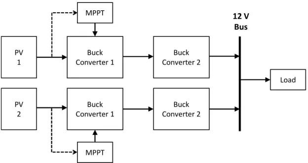
Figure 3-1 illustrates the simplified block diagram of the proposed Multiple Input Single Output (MISO) system with Maximum Power Point Tracker (MPPT) controller. The nominal input voltage chosen for the DC-DC Converter block is 24V. Renewable energy sources such as photovoltaics(PV) provide the input voltage in in the actual system and therefore will vary depending on the operating condition of the source. The DC-DC converter is designed to output nominal average output voltage of 12V at any current that is most efficient for the PV. This allows the use of step-down or Buck converter for the DC-DC converters.

Figure 3-1. Level 0 block diagram of the proposed system.

11

Figure 3-2. Level 1 block diagram of the proposed system.

The proposed converter will be designed to be a modular buck converter where each converter is capable of supplying varying amount of current for each converter up to their rated value. The input voltage specification of the first converter with MPPT will be between 17V and 40 V which will be the output voltage range of the PV source. By utilizing the MPPT, the first converter enables maximum output power to be drawn from the PV. This consequently produces output voltage that will vary; hence, the need for the second buck converter. The output voltage of the second converter will sit at 12 V. The total output power of the converter will be selected at 60W. This output power level is selected as this project is primarily a proof of concept and a lower operating power allows for a low cost hardware prototype to construct, including those of the PV sources that can be purchased off the shelf. In order to demonstrate the maximum operating points of the sources in supplying the total power, two PV sources with their corresponding converters will be designed and constructed for this thesis.Table 3-1 provides the summary of design requirements in this thesis.

12

Table 3-1. Summary of Design Requirements

Specification Value Justification

Total Output Power 60W The lower range of the converter is meant as a proof of concept for use with off the shelf PV

Input Voltage 17-40V This range of input voltages allows for the compatibility with 24V solar panels depending on load

DC Bus Voltage 12V A 12V bus is common and practical for most DC applications

13 Chapter 4

System Design and Simulation

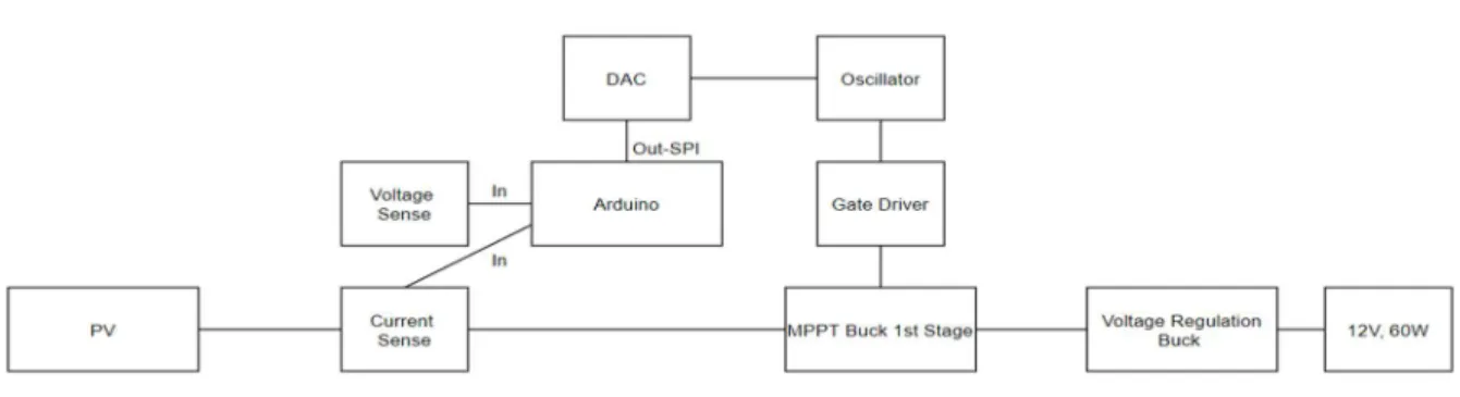
This chapter will be going through the design and simulation of the proposed system. Figure 4-1 is the block diagram of the total system.

Figure 4-1. Low Level Block Diagram of a Single Converter.

The converter designed has two step-down stages; therefore, there are two buck converter designs to consider. The design of the first stage involves choosing the MPPT buck converter controller. Currently, there are no MPPT buck converters that do not revolve around charging a battery; hence, the first buck converter is controlled through a microprocessor. The decision making for the microprocessor was primarily ease of use. The simplest microprocessor to use with plenty of documentation is the Arduino, with the main drawback being that the processor by itself may not be enough to drive the MPPT stage.

4.1 Component Selection

14

operates up to 60V, enough to account for any input spikes from the input of the solar panel and can allow for a full pass through. The output of the gate driver will match the timings of the input within 10nS, giving plenty of headroom for operation at 300kHz.

Figure 4-2. Rise/Fall Time of the LTC7004 [14].

The power used by the gate driver IC is miniscule as the total current needed to operate is around 225µA, with minimal external components to use; thus, simplifying its implementation. In order to operate the IC as a switch-mode gate driver, there only needs to be a bootstrap diode and capacitor necessary to drive the switch as shown in Figure 4-3. In order to select the bootstrap diode and capacitor, the bootstrap functions as an energy storage loop in order to drive a high side switch. The amount of current that runs through both components is very low, approximately 100mA; however, the voltage that each component will see across will be greater than the input voltage. This is due to how charge is built up in the capacitor, increasing its voltage in order to turn on the high side switch.

15

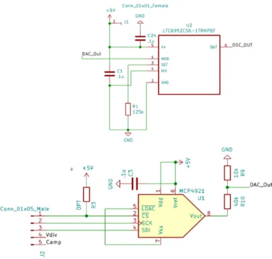
The Arduino cannot provide the input to the gate driver alone and requires additional components which were chosen based on practicality, ease of implementation and availability. The Arduino cannot provide any sort of square wave greater than 10kHz; and thus, an oscillator is chosen. Selecting a switching frequency greater than 10kHz allows for physically smaller component selection and a higher efficiency. The frequency driver chosen for the input of the MPPT gate driver is the LTC6992-1 as shown in Figure 4-4, with frequency set by a resistor and voltage-controlled duty cycle. The LTC6992-1 is chosen as it is relatively simple to implement, with just a resistor and a capacitor needed to set the output frequency, and a DC voltage to control the duty cycle.

Figure 4-4. LTC6992-1 Setup [15].

While the IC has a divider setting, the operating frequency is low enough such that it is not necessary to use a divider, therefore the divider pin is simply shorted to ground. In order to set the operating frequency, RSET

is chosen based on the following equation:

𝑅 = ∙ , where N = 1, and X = 350 kHz Eqn. 4-1

16

In order to control the duty cycle of the output, an input voltage between 0-1 volt is necessary. At 0V, the output is ground, and at 1V, the output is at 100% duty cycle. The Arduino can’t provide a controllable voltage between 0 and 1V and requires a separate source. Therefore, a digital to analog converter (DAC) fully operates the gate driver. The digital to analog converter communicates with the Arduino in order to provide a DC voltage which in turn drives the LTC6992-1.

The MCP4921 DAC was chosen based on its ease of use, 12-bit resolution, and 5V compatibility with the rest of the board. The MCP4921 has a Serial Peripheral Interface (SPI) instead of an Inter-Integrated Circuit (I2_{C) communication protocol, which allows for ease of use. I}2_{C requires pull up resistors}

and operates slower compared to SPI, which does not require any form of pull up resistor. This reduces the number of components needed to drive the MCP4921, making it easier to use. Secondly, the DAC has a 12-bit resolution, meaning if VREF is held to 1V through a resistor divider, the minimum step the DAC has

between 0 and 1V is as follows:

𝑉 = , where VRef is 1V Eqn. 4-3

𝑉 = 0.245𝑚𝑉 Eqn. 4-4

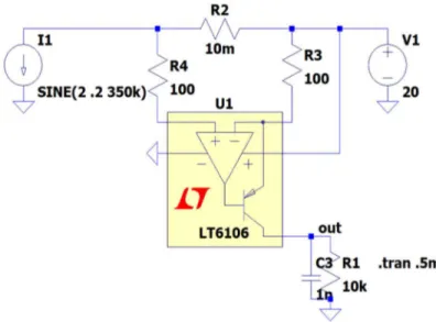
The components that have been discussed for the first stage have all been necessary to drive the gate driver; however, in order to implement the MPPT, the Arduino needs to read in feedback from the input of the converter. This is done by implementing a current sensor as well as a voltage sensor in order to calculate the power delivered to the converter. The current sensor revolves around using a low ohmage sensing resistor as well as an amplifier. The amplifier chosen is the LT6106 as shown in Figure 4-5 due to its simple implementation, with only two resistors needed to set the gain.

17 𝜏 =

∗ , where R = 10kΩ and C = 1nF  𝜏 = 16𝐾𝐻𝑧 Eqn. 4-5

Figure 4-5. LT6106 Standard Configuration [17].

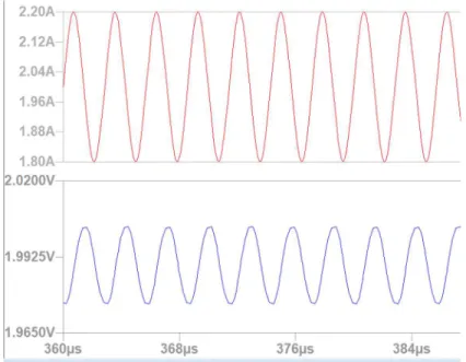
The capacitor is chosen to be 1nF as this allows for faster response on the output as well as still greatly filtering the output. Simulation with and without the output filtering shows that the output filtering reduces peak to peak noise by 30mV, which will assist in more accurate power readings for the Arduino.

18

Figure 4-7. Current Sense Output with Filtering

Figure 4-8. Current Sense Output without filtering.

The resistor on the output and resistor in series to –IN sets the gain for the amplifier with Eqn. 4-5:

𝐺𝑎𝑖𝑛 = 𝑅

𝑅 =

10𝑘𝛺 100𝛺= 100

19

With the gain chosen as 100 and the maximum input current that can be read on the Arduino at 5A, the sense resistor is chosen at 10mΩ, such that on the output, the relationship between input current

and output current is represented as = .

A resistive voltage divider is chosen to sense the input voltage. Since the maximum input voltage given in specification is 40V, then the maximum input voltage to the Arduino at that input should only be 5V. Thus, if R2 for a voltage divider is chosen at 10kΩ, then the respective R1 is calculated at 40kΩ.

The next step in the design is choosing the controller for the second stage of the converter. Since this stage functions as voltage regulation, a standard buck converter is satisfactory. The LT3864 is chosen as it has a 100% duty cycle pass through, which can be used if the input voltage is close to the output voltage. The evaluation board, DC2434A, has the input and output rating specifications required for the second stage buck converter. Therefore, the evaluation board itself will be used for the second stage output regulation.

The first component that needs to be sized is the inductor. Sizing the inductor value involves the operating frequency, expected input/output voltages as well as the maximum output current of the converter. The following equations are needed in order to find the inductor value for both converters. Once the value is found, generally, the component value is sized up, such that even when current saturates the inductance, the minimum inductance requirement is met to ensure the successful operation of the converter.

Duty Cycle = 𝐷 =𝑉𝑜𝑢𝑡 𝑉𝑖𝑛

Eqn. 4-7

Critical Inductance = 𝐿 =(𝑉 − 𝑉 )𝐷 𝛥𝑖 𝑓

Eqn. 4-8

20

The next components that are sized in both buck converters are the input and output capacitors. These are designed to combat ripple voltage expected on both input and output. Following the Buck topology, the output capacitor value depends on the inductor value, whereas the input capacitor does not. Eqn. 4-9 and 4-10 were used to solve for both the input and output capacitor values, respectively.

𝐶 = (1 − 𝐷) %𝛥𝑉 𝐿 ∗ 𝑓

Eqn. 4-9

𝐶 =𝐷(1 − 𝐷)𝐼

𝛥𝑉 𝑓 , where I is the maximum average output current

Eqn. 4-10

Once the component values for the power stage of both converters are found, the second step is to rate various components for the rest of the converter. This step ensures that components are chosen such that maximum rated voltage, power and current ratings are large enough for the components not to fail preemptively and allow for a longer life.

When sizing the inductor, two major considerations for an inductor will be its DC resistance and maximum peak (saturation) current. The maximum inductor current is calculated below to determine the saturation current rating of the inductor.

𝐼 = 𝐼 +𝑉(1 − 𝐷) 2𝐿𝑓

21

Figure 4-9. Inductance and temperature relative to current [18].

When an inductor saturates, the inductor begins to behave more resistively, but more importantly inductance reduces, which can be seen in Figure 4-5. Selecting an inductor with a saturation rating approximately 1.5 times greater than the theoretical peak current reduces the effect of saturation as well as maintaining minimum inductance (as mentioned above) at max operating conditions. The series DC resistance (DCR) of the inductor is important since it will affect the inductor’s conduction loss. Choosing an inductor with as low of a DCR as possible will improve efficiency.

To size and select capacitors, there are two considerations, the voltage rating of the capacitor and its equivalent series resistance (ESR). The voltage rating is chosen based on the peak voltage that is seen across the capacitor, which should be 1.5 or 2 times greater in the case of a large voltage spike through the capacitor. Secondly, because the capacitors are placed in parallel across the input and output, the ESR of the capacitor contributes to the voltage ripple seen on the input and output of the converter. The greater the ESR, the greater the ripple voltage. Therefore, on both input and output sides, it will be beneficial to place multiple capacitors in parallel to bring the total ESR down.

22

𝑃 = 𝐼 𝑅 Eqn. 4-12

The final components to size are the switches (MOSFETs) and diodes of the converter. For these components, the two main ratings are their peak voltage and average current rating. For the Buck converter, the maximum voltage across the high side MOSFET and the diode is equal to the input supply voltage. However, possible ringing can occur across the MOSFET due to parasitic inductance and capacitance on traces connecting to the switch. Therefore, the voltage rating of both components should also be at least 1.5x higher than the supply voltage across then switch. The difference between the MOSFET and the diode is their current, whose average values are calculated as follows:

𝐼 = 𝐼 ∗ 𝐷 Eqn. 4-13

𝐼 = 𝐼 (1 − 𝐷) Eqn. 4-14

4.2 Board Design

Once all components are selected, board design follows. For this thesis, the design of only the first stage of the system is realized as the second stage utilizes a commercially available demo board. The demo board is chosen as it is already rated to run at 12V output with an input voltage between 12V and 55V. The rated current for the components on the demo board are 5A, which meets the rated output current of the proposed system.

23

24

25

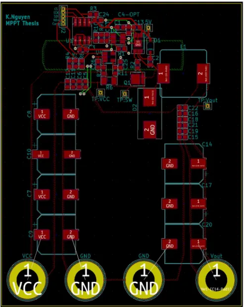
Figure 4-11. Layout of the First Stage.

4.3 Simulation Results

26

The initial simulation that was done in Simulink was to provide proof of concept for how well the MPPT algorithm would perform with an additional voltage regulation stage as well as a fixed resistive load. Figure 4-8 shows the model that is used to represent both stages in parallel.

Figure 4-12. Simulink Model of the Parallel Converters.

27

Figure 4-13. Current Sharing between two converters.

Secondly, the MPPT stage is important as the power from the solar panel is processed through the MPPT stage before the voltage regulation stage. When connecting the second stage directly to the PV, it is noticed that the second stage does not regulate the output voltage as well as if the MPPT stage is in between the PV and second stage. At the same irradiance on the input of both converters, there is no output voltage. The irradiance on the input needed to be increased for the same load as when there is an MPPT stage. Another concern is that both stages reduces the overall efficiency of the system, however, the overall efficiency that is reduced is better found through the second simulation; however, it can still be gleaned that the first stage is necessary.

Thirdly, when the load draws close to the max power of both inputs, the MPPT acts as a passthrough. This drives home the point that regardless of being a pass-through stage, the first stage can still provide regulation for the second stage.

28

is a current differential and thus a power differential. Secondly, it is noticed that when the MPPT stage is used, the system is able to provide a higher output power than without an MPPT stage.

The second simulation is done in LTSpice to ensure that the converter will work through both the first and second stage at various operating points. The first stage is tested without the DAC, which is replaced with an ideal voltage source instead. Overall, simulations with just the first stage are as expected, with the gate driver following the LTC6992-1 closely, as seen in Figure 4-10, where blue is the gate driver voltage and green is the output of the LTC6992-1. With non-ideal components, the efficiency of the buck converter is above 93% at full load.

Figure 4-14. Schematic of the First Stage.

29

Additional information to obtain through simulation includes understanding the relationship between the input of the LTC6992-1 and the duty cycle of the gate driver in order to fine tune the software driving the oscillator. Voltage ranges at 0.4V and 0.7V are sampled at steps of 10mV to observe the input/output relationship. Table 4-1 lists the relationship between the input to LTC6992-1, the change in duty cycle and period. A linear relationship between modulation voltage and duty cycle can be assumed based on this table along with an average variation at each step.

∆𝐷𝐶

𝛥𝑚𝑉= .00125 ± .00018 average change in duty cyle per 1 mV

Eqn. 4-15

∆𝑇

𝛥𝑚𝑉= 0.00344 ± µs average change in Time On period per 1 mV

Eqn. 4-16

Table 4-1. Relationship Between Modulation Voltage, Period, and Duty Cycle

Modulation Voltage (V) Time on Period (µs) Duty Cycle (unitless)

0.4 1.0651 14.2857

0.41 1.097 14.6429

0.42 1.127 15.0

0.43 1.16 15.3571

0.69 2.074 24.6429

0.7 2.1166 25.0

0.71 2.143 25.3571

0.72 2.18 25.7143

30

To extend this simulation to represent the real world, the MCP4921 LSB is defined at ~0.25mV, thus the average change in duty cycle and period can be related to the DAC:

∆𝐷𝐶

𝛥𝐿𝑆𝐵= 31𝑚 ± 45𝑚 average change in duty cycle per LSB of the DAC

Eqn. 4-15

∆𝑇

𝛥𝑚𝑉= 860 ± 117 𝑛𝑠 average change in TimeON per LSB of the DAC

Eqn. 4-16

This relationship allows us to understand that there will be plenty of available resolution from the DAC in order to precisely drive the first stage buck converter.

The second stage is simulated separately from the first stage. It is based off the LT3846 evaluation board, as seen in Figure 4-15. Components in LTSpice are changed based on values of the DC2434A evaluation board. The second stage is tested with a broad set of operating conditions such as the lowest input voltage at 12V and full load at 5A which would still regulate the output voltage. This gives a better idea of the overall efficiency of the system compared to the Simulink simulations and what additional requirements are needed to the MPPT algorithm in order to maintain proper regulation through both converters.

31

The second stage lowest input voltage that maintains a regulated output voltage at full load can be as low as 12V with a simulated efficiency of 99%. This is simply because the converter is operating as a pass through, and any loss occurs from the inductor and sense resistor in series with the output. When the converter is operating nominally at 24V, the efficiency decreases to 95% efficiency under full load.

32

Table 4-2. Simulation Results of the Proposed System at Various Operating Conditions

Modulation(V) 1st Output(V) 2nd Output (V) Total Efficiency

0.4 12.8 11.97 92.3077

0.6 21.77 11.974 93.2792

0.8 30.825 11.974 91.4216

1 Vin 11.974 94.6372

A point of interest is when operating the first stage, in Figure 4-14 as a pass through, the output voltage of first stage goes through an underdamped response as seen in Figure 4-17. The red waveform is the gate driver of the first stage, with the green waveform as the output of the first stage. Notice that while the gate driver acts as a pass-through switch, the output of the first stage rings for quite a while. The purple waveform is the output voltage. Since simulation only observed a few milliseconds at the start-up of each converter, this could explain why the first stage could improve the second stage near start up, as observed in the Simulink model.

33

Once the verification of a single converter is completed, converters are tested in parallel. To simulate different operating conditions of solar panels, the input voltage to the total converter will be different as well as the modulation voltage between each converter. However, current sharing is not expected in this neither voltage sources can be power limited like in Simulink. An example of both converters at full load in parallel is shown in Figure 4-18.

Both converters are operating under nominal conditions, with different duty cycles on the first stage. Voltage of both outputs regulate to 12V with current not being shared evenly, as shown in Figure 4-14. The blue waveform current out of the converter with the first stage at a duty cycle of 0.5 and the green waveform has the first stage operating at a duty cycle of 0.75. The currents of both converters are 4.513A and 4.723A, respectively.

34

Figure 4-19. Output Current Shared.

Next, boundary conditions are explored, where one converter is operating at close to pass through while the other is not, and by varying duty cycles. Once steady state is reached, it is observed that the converter with the higher duty cycle, will carry more current regardless of the voltage on the input of the converter. The parallel operation of the converters is proven to work provided enough power; however, since there is not a practical nor quick way to simulate a PV within LTspice with known open circuit voltages and short circuit current, hardware testing is needed to verify both Simulink and LTspice models.

4.4 Software Definition

35

36 Chapter 5

Hardware Testing and Results

After the design of the boards, the next step is to physically construct both boards and program them. Additionally, since the irradiance of solar panels varies when out in sunlight and does not provide a controlled test setup, two Rigol-DP832 power supplies are programmed to behave as solar panels. An electronic load and multimeters are used to control the load and measure the power on the output. The block diagram of the test setup is shown in Figure 5-1, with the physical test setup in Figure 5-2. Tests are performed with and without the maximum power point stage in order to compare the performance of DC-DC converters under the two scenarios.

37

Figure 5-2. Hardware Setup of both MPPT Boards.

5.1 System Construction:

38

Figure 5-3. A string of the MPPT System with Output Voltage Regulation Stage.

39

Figure 5-4. Updated Fractional Open Circuit Algorithm for the Arduino.

5.2 Test Setup and Results:

40

Figure 5-5. Varying I-V Irradiance Curves [13].

Each of these varying irradiance curves will have different power curves related to it as well as different MPPs. Figure 5-6 references back to Figure 5-5, except that it relates the different irradiances to power and voltage.

41

It is important to note about the behavior of solar panels that the resistive load on the output of the solar panel will determine its operating current and voltage, and therefore its operating power. This means that each resistance has their own unique current and voltage, in other words, once the entire system gets loaded, each PV or input will have a different resistance based on the load. Programming the Rigol-DP832 means that an irradiance curve needs to be loaded to the power supply and then tracked depending on what output resistance and power the power supply reads. The algorithm for how the power supply operates is shown in Figure 5-7.

Figure 5-7. Solar Panel Algorithm used with the Rigol.

42

operate at. Once achieved, the power supply will track the resistance that the converter sees based on Ohm’s law to operate on the irradiance curve that it expects.

The different irradiance curves that were programmed into the power supply are shown in Figures 5-8 and 5-9 with their corresponding IV and power curves. Table 5.1 more accurately details the open circuit voltage, short circuit current, the MPP (Maximum Power Point), and the voltage at the MPP. Using these values, a curve can be generated to track a solar panel at varying irradiances. Comparing Figures 5-8 and 5-9 to Figures 5-5 and 5-6 shows that three points can be used to match the IV and power curve very well.

43

Figure 5-9. Power Curves at 3 Different Power Points used with the Rigol.

Table 5-1. Irradiance Curve Points

Maximum Power

(W) Open Circuit Voltage (V) Short Circuit Current (A) Voltage at MPP (V) Resistance at MPP (Ω)

65 30 2.55 25.5 10.00

55 28 2.45 22.4 9.123

45 26 2.31 19.5 8.45

44

45

Table 5-2. Test Results with MPPT Stage

1: MPP (W) Vin (V) Iin (A) Iout (A) Res (Ω) Pin (W) Pout Efficiency (%)

P1 65 26.47 2.00 4.389 13.32 52.675 108W

at 9A,12V

93.49

P2 65 25.65 2.44 4.611 10.49 62.84

2:

P1 65 28.61 0.77 1.71 39.735 22.316 48W

at 4A,12V

93.09

P2 65 28.39 1.03 2.29 31.185 29.242

3:

P1 55 22.92 2.20 3.943 10.39 50.424 102W

at 8.5A,12V

92.00

P2 65 26.01 2.24 4.556 11.60 58.262

4:

P1 45 19.71 1.84 2.85 9.16 36.524 91.2W

at 7.6A,12V

93.70

P2 65 26.55 2.28 4.75 13.65 60.80

46

system to provide the additional power. The MPPT stage in both Test 2 examines the converter’s operation when the power needed from the load is far less than the maximum power point. In this case, where the load isn’t as demanding, both converters share similar amounts of power. Test 4 examines a drastic difference in the operating power, yet still close to the maximum load available. Test 4 has the correct resistances at which the converters should operate; however, the current that each is supplying is incorrect and it does not track with the solar panel. The ideal power that the two converters should have been operating are approximately 44W and 52W, or 19.71V at 2.236A and 26.55V at 1.95A. This limitation is most likely due to the operating conditions of the power supply itself and its inability to emulate the IV characteristics of a real solar panel.

Figure 5-10 shows the test setup without the MMPT board. This is done by tying the DC-DC converters directly to the Rigols. The same test cases from above are repeated and the results are listed in Table 5-3.

47

Table 5-3. Test Results without the MPPT Stage

1: MPP (W) Vin (V) Iin (A) Iout (A) Res (Ω)

Pin (W) Pout Efficiency (%)

P1 65 26.23 2.22 4.522 11.81 55.708 108W

at 9A,12V

95.27

P2 65 26.26 2.10 4.45 12.486 55.146

2:

P1 65 28.56 0.83 1.91 33.521 24.276 48W

at 4A,12V

94.80

P2 65 28.30 0.93 2.09 30.38 26.356

3:

P1 55 22.41 2.44 4.36 9.16 54.90 102W

at 8.5A,12V

95.43

P2 65 26.51 1.96 4.13 13.53 51.98

4:*

P1 45 19.51 2.3 3.56 8.52 44.678 84W

at 7.0A,12V

95.84

P2 65 27.19 1.58 3.43 17.16 42.96

*This test case only ran up to 7A before the output drops out

48

converter only regulates the output voltage, in Test setup 2 when there is an input power less than 50% of the load power demanded, the buck converter drops out as it cannot regulate the input power to provide the demanded power. Therefore, without the MPPT stage, the two buck converters cannot operate with large differences in current, nor large differences in input power. Compared to Table 5-2, the system draws a more uneven split of current with the most uneven split occurring at 25% from the midpoint current as resulted in Test 4. Figure 5-11 and 5-12 show the differences in current sharing between both cases. From these figures, we can see that in the first test setup, there is larger variation in output current, whereas in the second test setup all output currents tend to be near each other.

49

Figure 5-12. Comparison of Output Currents in Setup 2 w/o the MPPT Stage.

50

Figure 5-13. Efficiency Comparison of Test Setup 1 w/MPPT and 2 w/o MPPT.

51 Chapter 6

Conclusion

This thesis entails the study of utilizing the MPPT controller in a multiple input single output system. Hardware tests were conducted to demonstrate the overall performance of using the MPPT before the main converters when sharing the same load. Results from hardware testing show the benefit of using the MPPT as the pre-regulation stage in allowing for more power from the source to be used efficiently.

The study conducted in this thesis provides proof of concept that without the MPPT stage, power would be limited by the smallest available power source. Incorporating the MPPT stage in the system allows for additional power from the source and prevents the power source with lowest amount of power from limiting the system. Results also indicate that the MPPT stage are most beneficial when the power differential between solar panels is the greatest. Furthermore, even with the additional components in the system as a trade-off, the test results show insignificant decrease in the overall efficiency of the system of about 2-3%. This project can be improved with better testing setups, algorithms, and a board redesign.

Follow up work from this thesis may include redesigning and improving the board. Fixing the current sense amplifier is key as this would allow for better algorithms to be used, such as the Perturb and Observe or the Incremental Conductance methods. Using a more enhanced different algorithm allows for a better power point tracking which consequently may result in higher output power. The output from each board can also be combined with a better method than using the OR diode method. This is especially important with large power applications since at max load, the Schottky diodes currently used in this thesis consume 3.3W which worsen as output current requirement increases. One method to combat this is to use MOSFET that has much less on resistance and thus may significantly reduce power loss.

52

the buck-boost topology. This allows for the MPPT stage on the input to have a wide range of duty cycle even and for the input voltage to be below the expected output voltage. With the existing board which implements the buck topology, the input voltage to the second converter needs to be greater than 12V. A buck-boost allows for a step up in case the initial stage steps down the input too much, allowing for more versatility.

Another improvement that could be made is by testing the proposed system with actual solar panels. The power supply used in this thesis can only simulate solar panels with limited operating characteristics. Using a solar panel under controlled lighting would be the ideal way to test system, allowing for different panels to obtain different amounts of light such as to test an unbalanced system.

53

BIBLIOGRAPHY

[1]B. Hachim, D. Dahlioui and A. Barhdadi, "Electrification of Rural and Arid Areas by Solar Energy Applications," 2018 6th International Renewable and Sustainable Energy Conference (IRSEC), Rabat, Morocco, 2018, pp. 1-4.

[2] A. Beaudet, "How do I read the solar panel specifications? | Solar Power News & DIY Solar Tips", Solar Power News & DIY Solar Tips, 2019. [Online]. Available:

https://www.altestore.com/blog/2016/04/how-do-i-read-specifications-of-my-solar-panel/. https://www.altestore.com/blog/2016/04/how-do-i-read-specifications-of-my-solar-panel/

[3] A. Faizan, “Induction Generator: Types & Working Principle: Permanent Magnet Generator Working Principle,” Electrical Academia, 18-Aug-2018. [Online]. Available:

http://electricalacademia.com/induction-motor/induction-generator-types-working-principle-permanent-magnet-generator-working-principle/.

http://electricalacademia.com/induction-motor/induction-generator-types-working-principle-permanent-magnet-generator-working-principle/

[4]S. S. Gite and S. H. Pawar, "Modeling of wind energy system with MPPT control for DC microgrid," 2017 Second International Conference on Electrical, Computer and Communication Technologies (ICECCT), Coimbatore, 2017, pp. 1-6.

[5] "Microhydropower Systems", Energy.gov, 2019. [Online]. Available:

https://www.energy.gov/energysaver/buying-and-making-electricity/microhydropower-systems. [6]" Heat Dissipation for Morningstar's TriStar Controllers", Morningstar Corporation, 2019. [Online]. Available: https://www.morningstarcorp.com/landing_page/download-white-paper-morningstars-trakstar-mppt-technology-maximum-input-power/#gf_45.

[7] "MPPT Algorithm", Mathworks.com, 2019. [Online]. Available:

https://www.mathworks.com/solutions/power-electronics-control/mppt-algorithm.html. [Accessed: 26- Dec- 2019].

[8] Rawat, Rahul & Chandel, Shyam. (2013). Hill climbing techniques for tracking maximum power point in solar photovoltaic systems - A review. Special Issue of International Journal of Sustainable Development and Green Economics. 2. 90-95.

https://www.researchgate.net/publication/288128372_Hill_climbing_techniques_for_tracking_maximum_p ower_point_in_solar_photovoltaic_systems_-_A_review

[9]B. Guo, S. Bacha, M. Alamir and H. Imanein, "An anti-disturbance ADRC based MPPT for variable speed micro-hydropower plant," IECON 2017 - 43rd Annual Conference of the IEEE Industrial Electronics Society, Beijing, 2017, pp. 1783-1789.

[10] S. Baroi, P. C. Sarker and S. Baroi, "An Improved MPPT Technique – Alternative to Fractional Open Circuit Voltage Method," 2017 2nd International Conference on Electrical & Electronic Engineering (ICEEE), Rajshahi, 2017, pp. 1-4.

54

[12] T. Taufik, K. Htoo and G. Larson, "Multiple-input bridge converter for connecting multiple renewable energy sources to a DC system," 2016 Future Technologies Conference (FTC), San Francisco, CA, 2016, pp. 444-449, doi: 10.1109/FTC.2016.7821646.

[13] Yau, Her-Terng & Lin, Chih-Jer & Liang, Qin-Cheng. (2013) PSO Based PI Controller Design for a Solar Charger System. TheScientificWorldJournal. 2013

[14] Analog.com. 2020. LTC7004. [online] Available : https://www.analog.com/media/en/technical-documentation/data-sheets/LTC7004.pdf

[15] ROHM TECH WEB: Technical Information Site of Power Supply Design. 2020. Switching Regulator Basics: Bootstrap | Basic Knowledge | ROHM TECH WEB: Technical Information Site Of Power Supply Design. [online] Available at: https://techweb.rohm.com/knowledge/dcdc/dcdc_sr/dcdc_sr01/829 [16] Analog.com. 2020. LTC6992. [online] Available : https://www.analog.com/media/en/technical-documentation/data-sheets/LTC6992-1-6992-2-6992-3-6992-4.pdf

[17] Analog.com. 2020. LT6106. [online] Available: https://www.analog.com/media/en/technical-documentation/data-sheets/6106fb.pdf

55 Appendix A: Rigol DP-832: Solar Panel Code

%Create VISA object

dp800 = visa( 'ni','USB0::0x1AB1::0x0E11::DP8C163352016::INSTR' ); dp801 = visa('ni', 'USB0::0x1AB1::0x0E11::DP8C163352091::INSTR'); %Panel 1: Setting the Irradiance Curve

Voc = 26.0; Isc = 2.31; Vmpp = 19.5; MP = 45.0;

%Finding the points along the Curve Res = zeros(1,(Voc*100));

PowerCurve = zeros(1,(Voc*100)); Ilimit = MP/Voc;

Slope = Isc/(Vmpp-Voc); Yint = -1*(Voc)*Slope; %Generate Lookup Table

%volts = linspace(0,Voc,(Voc*10)+1);

for x = 1:(Voc*100)-1 if x <= Vmpp*100 current = 2.5; else

current = ((x/100)*(Slope) + Yint); end

Res(x) = x/100/current;

PowerCurve(x) = round(x/100*current, 1); end

%Do the same with the second power supply Voc2 = 30.0;

Isc2 = 2.55; Vmpp2 =25.5; MP2 = 65.0;

Res2 = zeros(1,(Voc2*100));

56 Ilimit2 = MP2/Voc2;

Slope2 = Isc2/(Vmpp2-Voc2); Yint2 = -1*(Voc2)*Slope2;

for x = 1:(Voc2*100)-1 if x <= Vmpp2*100 current = 2.5; else

current = ((x/100)*(Slope2) + Yint2);

end

PowerCurve2(x) = round(x/100*current,1); Res2(x) = x/100/current;

end

n = 0; %Used to generate an infinite loop %opens both instruments for communication fopen(dp800);

fopen(dp801);

%initiate both panels, both on with maximum power point at Voc MaxCurrent1= MP/Voc;

fprintf(dp800, ':INST CH1');

fprintf(dp800, [':VOLT',' ',num2str(Voc)]);

fprintf(dp800, [':CURR',' ', num2str(MaxCurrent1)]);%fix

MaxCurrent2 = MP2/Voc2; fprintf(dp801, ':INST CH1');

fprintf(dp801, [':VOLT',' ',num2str(Voc2)]); fprintf(dp801, [':CURR',' ', num2str(MaxCurrent2)]);

57 while flag == 0; % allow the the system to stablize

fprintf(dp800, ':MEAS:POWER? CH1'); InitialPower1 = fscanf(dp800);

InitialPower1 = str2num(InitialPower1); fprintf(dp801, ':MEAS:POWER? CH1'); InitialPower2 = fscanf(dp801);

InitialPower2 = str2num(InitialPower2);

if InitialPower1 > 10 && InitialPower2 > 10 flag = 1;

end end

%get on the IV curve from the power curve

InitialPower1 = round(InitialPower1,1); InitialPower2 = round(InitialPower2,1);

NewV1 = find(PowerCurve >= (InitialPower1-.1)

& PowerCurve<= (InitialPower1+0.1),1,'last')/100; NewV2 = find(PowerCurve2 >= (InitialPower2-0.1)

& PowerCurve2 <= (InitialPower2 + 0.1),1,'last')/100;

%set current and voltage limit for power curve fprintf(dp800, ':INST CH1')

fprintf(dp800, [':VOLT',' ',num2str(NewV1)]); fprintf(dp800, [':CURR',' ', num2str(Isc+0.05)]);%fix

%set the second 1

fprintf(dp801, ':INST CH1')

fprintf(dp801, [':VOLT',' ',num2str(NewV2)]); fprintf(dp801, [':CURR',' ', num2str(Isc2+0.05)]);

58 %find the current

Inew = str2num(FindCurrent(dp800,1)); Inew2 = str2num(FindCurrent(dp801,1));

%Use found current to find resistance %if current is zero set to Voc

if Inew <= 0.005 Vpoint = Voc; else

Vpoint = find( Res < (Vpoint/Inew)+0.1 & Res > (Vpoint/Inew)-0.1, 1 )/100; end

if Inew2 <= 0.005 Vpoint2 = Voc2; Else

%finds the voltage to be set to from the current Vpoint2 = find( Res2 < (Vpoint2/Inew2)+0.1

& Res2 > (Vpoint2/Inew2)-0.1, 1 )/100; End

%Set the new voltages,

fprintf(dp801, [':VOLT',' ',num2str(Vpoint2)]); fprintf(dp800, [':VOLT',' ',num2str(Vpoint)]); pause(3);

end

%Find Voltage based on which instrument or channel function voltage = FindVoltage(dp800,channel)

fprintf(dp800, [':MEAS:VOLT:DC?', ' ','CH', num2str(channel)] ); %Send request voltage = fscanf(dp800);

End

function current = FindCurrent(dp800,channel) %same as above

fprintf(dp800, [':MEAS:CURR:DC?', ' ','CH', num2str(channel)] ); %Send request current = fscanf(dp800); %Read data

59 Appendix B: Arduino Code:

#include <SPI.h>

int j = 0;

int CurrentDC = 0; float Vtarget = 0; float Vin = 0;

void setup() {

SPI.begin();

analogReference(INTERNAL); Vtarget = FindVoltage(); Vtarget = CompareVoc(Vtarget); CurrentDC = DutyCycle(Vtarget); Serial.println(CurrentDC); write4921(CurrentDC);

}

void loop() { Vin = FindVoltage();

if (Vin <= (Vtarget+0.5) & Vin >= (Vtarget -0.5)){ write4921(CurrentDC);

}

else if (Vin > (Vtarget + 0.5)) { CurrentDC = CurrentDC - 10; write4921(CurrentDC); }

else {

CurrentDC = CurrentDC +10; write4921(CurrentDC); }

60 }

//Writes to the DAC void write4921(int value) { if (value >= 4000) value = 4000; if (value <= 100) value = 0; byte data;

data = highByte(value); data = B00001111 & data; data = B00110000 | data; digitalWrite(10, LOW); SPI.transfer (data); data = lowByte(value); SPI.transfer (data); digitalWrite(10, HIGH); }

//Uses a rolling filter to average voltage values float FindVoltage(){

int counter = 0; float Vout = 0;

float Vin[5] = {0,0,0,0,0};

for (int i = 0; i < 8; i++){

Vin[counter] = analogRead(A0); counter = counter +1;

if (counter == 5) counter = 0; //Serial.println(analogRead(A0)); }

Vout = Vin[0] + Vin[1] + Vin[2] + Vin[3] + Vin[4]; Vout = (Vout/5.0)*(83.2/1024.0);

Serial.println(Vout); return Vout;

}

61 int Vin = 0;

//Serial.println(voltage);

if (voltage <= 30.5 & voltage >= 29.0) return 25.5; // 65 watts if (voltage >= 27.5 & voltage <= 28.0) return 22.4; // 55 watts if (voltage >= 25.5 & voltage <= 26.5) return 19.5; // 45 watts if (voltage >= 24.5 & voltage <= 25.5) return 18.0; // 40 watts }

int DutyCycle(float Vin){

62 Appendix C: Bill of Materials

Value Package Size

Description Manufacturing Part Number

Manufacturer # to order per board # to order in total Unit Price Cost Per part MCP4 921-E/SN

8SOIC DAC MCP4921-E/SN Microchip Tech 2 4 1.97 7.88

LTC69

92-1 TSOT23 Voltage Controlled PWM

LTC6992-1 LTC 2 4 4.00 16

LTC70

04 10-MSOP Gate Driver LTC7004 LTC 2 4 5.75 23

LT610 6

TSOT23 Current Sense Amp

LT6106 LTC 2 4 2.18 8.72

CSD18 543Q3 A

3.3x3.3

mm Power Mosfet CSD18543Q3A TI 2 4 0.84 3.36

BAT4

6 SOD323 Bootstrap Diode BAT46WJ115 Nexperia 2 4 0.38 1.52

sk810 DO214A B

Power Diode SK810L-TP Micro Commerical

2 4 0.70 2.8

10u 13.5x12.

5 mm Inudctor SRP1265A-100M Bourns 1 3 1.68 5.04

125k 0603 Resistor

RC0603JR-070RL Yageo 2 3 0.38 1.14

0 0603 Resistor

RC0603JR-070RL Yageo 2 10 0.10 1

10k 0603 Resistor

RC0603JR-0710KL

Yageo 4 10 0.10 1

100k 0603 Resistor RT0603BRD071

00KL Yageo 2 5 0.38 1.9

750k 0603 Resistor

RC0603FR-07750KL Yageo 2 10 0.10 1

10m 1206 Resistor PF1206FRF070

R01L Yageo 2 4 0.54 2.16

100 0603 Resistor RT0603DRD071

00RL

Yageo 4 6 0.19 1.14

40k 0603 Resistor PAT0603E4002

BST1 Vishay 2 4 0.92 3.68

.1u 0603 Capacitor CC0603ZRY5V

9BB104 Yageo 9 18 0.10 1.8

10p 0603 Capacitor AC0603JRNPO0

BN100

Yageo 11 22 0.17 3.74

20u 10x10m

m Capacitor EEE-FK2A220 Panasonic 5 10 0.70 7

10u 10x10m

m

Capacitor EEE-FK1K100P Panasonic 4 10 0.62 6.2

63

pin Socket Electronics

1x5m m header

- Arduino

Header Pin PREC005SAAN-RC Sullins Connector Solutions

1 3 0.15 0.45

1mm