Analysis of complex survey samples.
Thomas Lumley
Department of Biostatistics
University of Washington
April 15, 2004
AbstractI present software for analysing complex survey samples in R. The sampling scheme can be explicitly described or represented by replication weights. Variance estimation uses either replication or linearisation.
1
Introduction
Analysis of complex survey samples has traditionally been the province of spe-cialised software. This is partly due to the computational burden of large sur-veys, but the philosophical separation between survey statistics and much of the rest of the discipline is also important. In most areas of statistics the data are regarded as random, and the statistician must model their distribution (or the distribution of statistics computed from them). In traditional ‘design-based’ survey statistics the population data are regarded as fixed and the randomness comes entirely from the sampling procedure.
The advantage of the design-based view is that the sampling procedure is under the control of the analyst, and can in principle be known perfectly, the exception to George Box’s dictum that all models are wrong.
In this paper I describe a package of R code for analysing complex surveys. Before describing the features of the package I will present a short overview of the methods used in the survey package. Books covering survey statistics in more detail include Cochran (1977) and Levy & Lemeshow (1999). Examples of analyses across multiple computer packages are given at http://www.ats. ucla.edu/stat/survey/survey_howtochoose.htm.
2
Statistical methods
In the case of simple random sampling from a large population a survey sample will be nearly an independent and identically distributed sample from an un-known distribution. The law of large numbers and central limit theorem justify most of the same analyses from a design-based viewpoint as they do from a model-based viewpoint.
The complications in a complex survey sample result from
stratification Dividing the population into relatively homogenous groups (strata) and sampling a predetermined number from each stratum will increase precision for a given sample size
clustering Dividing the population into groups and sampling from a random subset of these groups (eg geographical locations) will decrease precision for a given sample size but often increase precision for a given cost.
unequal sampling Sampling small subpopulations more heavily will tend to increase precision relative to a simple random sample of the same size.
finite population Sampling all of a population or stratum results in an esti-mate with no variability, and sampling a substantial fraction of a stratum results in decreased variability in comparison to a sample from an infinite population.
I have described these in terms of their effect on the design of the survey. More important to the programmer is their effect on the analysis. Analysing a stratified sample as if it were a simple random sample will overestimate the standard errors, analysing a cluster sample as if it were a simple random sam-ple will usually underestimate the standard errors, as will analysing an unequal probability sample as if it were a simple random sample. Note that the de-sign effectandmisspecification effect agree (qualitatively) for stratification and clustering but not for unequal probability sampling.
Clustering can be carried on to multiple levels: e.g., sampling individuals from families within neighbourhoods within cities. The largest clusters, which are sampled independently within a stratum, are called PSUs (primary sampling units). As they are sampled independently they are a fundamental part of the statistical analysis.
2.1
Weighting
When units are sampled with unequal probability it is necessary to give them correspondingly unequal weights in the analysis. Suppose 100 individuals are sampled from each state of the USA. The 100 people sampled from California represent a population of 34,000,000 people; the 100 sampled from Iowa repre-sent only 2,900,000 people. Thus, each Californian must receive nearly 12 times as much weight in a valid analysis.
Thisinverse-probability weightinghas generally the same effect on point esti-mates as the more familiar inverse-variance weighting, but very different effects on standard errors. In addition, the general principle in regression modelling that misspecified weights cause no bias does not apply here: it relies on the assumption that the model correctly specifies the mean, which is not permissi-ble in a design-based analysis. In some circumstances a model-based analysis may be able to omit the weights and thus gain more precision (DuMouchel & Duncan, 1983).
2.2
Variances
Two widely used and fairly general techniques for variance estimation are Taylor series linearisation and replication weights. The former is based on reducing the variance estimation problem to estimating the variance of a mean, the latter is based on the same ideas as the jackknife. These two approaches are discussed in more detail below and are implemented in thesurveypackage.
Other variance estimation techniques for surveys include the method of ran-dom groups and PSU-level bootstrapping. The method of ranran-dom groups is based on sampling within PSUs. It is described by Wolter (1985), a compre-hensive reference (at that date) on survey variance estimation. Bootstrapping at the PSU level, along with BRR and the jackknife methods, is discussed in Chapter 6 of Shao & Tu (1995).
2.2.1 Variances by linearisation
Taylor series linearisation estimators are very similar to the sandwich variance estimators widely used in biostatistics and econometrics. Survey-oriented pre-sentations of the theory are given by Binder (1983), and Chapter 6 of Wolter (1985).
The principle is simple. Consider estimating the variance of the population total of a variableY. WriteYsij for observation j in PSU i in stratums and πsij for its sampling probability.
Inverse-probability weighting gives a contribution to the total from each PSU Ysi·= X j 1 πsij Ysij,
and as PSUs are sampled independently within strata the variance of the stra-tum total can be estimated by the empirical variance of the PSU totals. Ifns
is the number of PSUs sampled in thenth stratum then Ys·· = ns X i=1 Ysi· ¯ Ys·· = 1 ns ns X i=1 Ysi· c var[ ¯Ys··] = 1 ns−1 ns X i=1 Ysi·−Y¯s·· 2 .
This variance will be too large when sampling an appreciable fraction of a population. When a simple random sample of PSUs is taken in each stratum, with no further subsampling, the variance can be multiplied by a finite popula-tion correcpopula-tion 1−fs, wherefsis the proportion of PSUs sampled in stratums.
For other sampling designs the correct finite population adjustments will differ. Bellhouse (1985) describes algorithms for doing this if the necessary design de-tails are available. A reviewer points out that in cases where finite-population
corrections are substantial it is also important to note that estimation usually assumes the PSUs are sampled with replacement, which is, of course, not typi-cally the case.
Finally, adding up estimates for each ofSstrata gives a total and an estimate of its variance: Y··· = S X s=1 Ys·· c var[Y···] = s X s=1 (1−fs) 1 ns−1 ns X i=1 Ysi·−Y¯s·· 2 .
Now, in most cases a statistic can be written as the solution ˆθof an estimat-ing equation
n X
i=1
U(Xi;θ) = 0
whereθ7→U(X;θ) is differentiable (a notable exception being quantiles). The varianceVU of
n X
i=1
U(Xi;θ)
can be estimated in the same way as the variance of any other population total, and an asymptotic approximation to the variance of ˆθis then
n X i=1 ∂Ui ∂θ !−1 VU n X i=1 ∂Ui ∂θ !−1 .
With inverse-probability weighting we estimateθby solving
n X 1=i ˜ Ui(Xi, θ) = n X i=1 1 πi U(Xi;θ) = 0
whereπi is the sampling probability for theith case. The asymptotic
approxi-mation to the variance of ˆθis then
n X i=1 ∂U˜i ∂θ !−1 VU˜ n X i=1 ∂U˜i ∂θ !−1 .
Estimating the variance of ˆθ is a matter of estimating the mean of ∂U /∂θ˜ and the variance of the mean of ˜U(θ) at ˆθ, which can be done using standard methods for means in complex samples.
Survey sampling implementations of these sandwich variances differ from those in other areas of statistics only in the handling of stratification and finite-population corrections. The resulting variance estimators are approximately unbiased but may be quite variable and as a result tend to lead to confidence intervals that are too short in small samples.
2.2.2 Variances by subsampling
A second class of variance estimators is based on the jackknife. Chapters 3 and 4 of Wolter (1985) discuss these estimators from a survey statistics viewpoint. A different viewpoint is presented in Chapter 6 of Shao & Tu (1995).
In unstratified surveys one PSU at a time is deleted and the others reweighted to keep the same total weight (known as theJK1jackknife). For stratified designs theJKnjackknife removes one PSU at a time, but reweights only the other PSUs in the same stratum.
The Balanced Repeated Replicates estimator is intended for surveys with ex-actly two PSUs in each stratum. Subsamples are constructed by giving weights of 2 to one PSU in a stratum and 0 to the other. While in principle the BRR estimator would require 2Lsets of computations forLstrata, it is possible to con-struct small, balanced sets of half-samples that give exactly the same variance for a linear statistic and similar variance for nonlinear statistics. These sets of replicates are constructed according to Plackett–Burman (Plackett & Burman, 1946) designs. The number of replicates in a Plackett–Burman design is always a multiple of four. It is conjectured that designs exist for any multiple of four, which would imply that at mostL+ 4 replicates are sufficient (known to be true forLup to 423). Given a design withmreplicates it is easy to construct one with 2m replicates, thus designs with at most 2L replicates can easily be provided. A library of Hadamard matrices, from which Plackett–Burman designs can be constructed, is available athttp://www.research.att.com/~njas/hadamard/ and Wolter (1985) provides designs form≤100.
Fay’s method (Judkins, 1990) is a modification of BRR where a parameter ρ∈[0,1) is chosen and weights of 2−ρandρare used for the two PSUs in each stratum. This has the advantage of using all the data and may give more stable estimates ifρis chosen correctly. Fay’s method reduces to BRR ifρ= 0.
As an alternative to replicates constructed by the analyst, some recent US government surveys provide replicate weights instead of information on PSUs. These replicate weights are typically generated by one of the methods described above, but may then be modified for various reasons. One important use of replicate weights is to preserve privacy: it may be possible to disguise the PSUs and so prevent the identification of individuals in small PSUs.
A general formula for variance estimation from replicate weights is var[ˆθ] =CX
i
ci(ˆθ(wi)−θ¯)⊗2 (1)
where⊗2 indicates the outer product of a vector with itself. Here ˆθ(wi) is the
estimate ofθ with the ith set of weights, ¯θis the average of the replicate esti-mates ofθ,ciis a replication-specific constant andCis an overall scaling factor.
The full-sample estimate ˆθis sometimes used instead of ¯θ. If the average weight for each observation is the same as its sampling weight there is no difference for linear statistics and it is not clear which is better for nonlinear statistics.
IfLis the number of strata,nthe total number of PSUs andnsthe number
C ci
JK1 (n−1)/n 1
JKn 1 (ns−1)/ns
BRR 1/L 1
Fay 1/(L(1−ρ)2) 1
Only the jackknife methods can readily incorporate a finite-population correc-tion. Each replicate is specific to a stratum, so the constantcican be multiplied
by the finite-population correction for that stratum.
2.3
Poststratification and raking
Stratified sampling requires a stratifiedsampling frame, that is, full prior knowl-edge of the stratum for every primary sampling unit in the population. It is often the case that the size of each population stratum is known (eg from Census data) and that the stratum for each sampled unit can be determined easily, but that a stratified sampling frame is prohibitively expensive.
Much of the efficiency of stratified sampling can then be recovered by scaling the sampling weights so that the total weight for each sample stratum is the same as the stratum size in the population. Variance estimation using replicate weights is still straightforward: the same scaling is performed on each set of replicates. Variances by linearisation are more complicated, at least in small samples.
In some situations the joint population distribution of a number of stratifying factors is not known but their marginal distributions are known. It would be desirable to post-stratify on each of these factors, but matching the marginal distribution of one factor may unmatch the marginal distribution of others. However, it is typically the case that iteratively post-stratifying on each factor in turn will lead to a converging sets of weights where the marginal distribution of each factor matches the population margins. This iterative algorithm is called
raking.
Convergence will always occur if the sample joint distribution of the factors has no empty cells. If there are empty cells then convergence will occur whenever there is a joint distribution with the desired margins and the same pattern of empty cells.
2.4
Subpopulations
A subpopulation of a survey cannot simply be treated as a smaller survey. The subpopulation may have fewer PSUs in some strata, resulting in a ran-dom, rather than fixed, sample size. Conceptually, the correct analysis involves keeping the entire sample but assigning zero weight to observations not in the subpopulation. This strategy maintains, for example, the equivalence between separate regression models in subpopulations and a common regression with interactions.
A subpopulation of a survey design specified by replicate weights, on the other hand, can simply be analysed as a subset. The replicate weights are based on the design of the full sample and are still correct.
There is a minor computational ambiguity in using zero weights versus sub-setting: should observations with no weight still contribute to constraints in constrained models? For example, in fitting a linear model to binomial data, should the coefficients be restricted so that fitted proportions are in [0,1] even for cases with zero weight? There is no entirely satisfactory answer, but it is cer-tainly simpler for cases with zero weight not to participate even in constraints.
3
The
survey
package
Thesurveypackage consists entirely of interpreted R code. This paper describes version 2.2. Future versions will be available at the Comprehensive R Archive Network (http://cran.r-project.org).
Thesurveypackage has two main purposes. The first is to bind the neces-sary design metadata to the data so that the correct analysis adjustments can be performed reliably and automatically. This is done by constructor functions svydesignand svrepdesign that create objects containing a data frame and design information. Extracting subsets of the data must preserve the meta-data and also allow for accurate subpopulation estimates, so methods for"[", subset,update, and thena.actioncommands are provided.
The second main purpose is to provide valid variance estimates for statistics computed on these objects. ThesvyCprodfunction abstracts the computations needed for Taylor series linearisation andsvrVardoes a similar job for replicate weights. ThewithReplicates()function computes replicate-weight variances for arbitrary statistics specified by functions or expressions.
Computation of the statistics themselves is performed largely by existing R functions, thesurveypackage merely providing wrappers. For example,svyglm andsvrepglm construct calls to glmto fit generalised linear models and then modify the resulting objects to give correct variances. This approach makes it easy to extend the package, at some cost in speed and memory use.
3.1
Sampling design and Taylor series linearisation
Thesvydesign function constructs an object that specifies the strata, PSUs, sampling weights or probabilities, and finite population correction for a survey sample.
The resulting objects can be used in the statistical functions whose names be-ginsvy: svymean,svyvar,svyquantile,svytable,svyglm,svycoxph,svymle. Standard errors are computed using Taylor series linearisation (where available). The modelling functionssvyglmandsvycoxphrequire that all the variables in the model are contained in the survey design object. This would be good practice in any case; it is required to avoid scoping problems, as these func-tions work by constructing and evaluating calls to the ordinaryglmandcoxph
functions.
Fairly general pseudolikelihood estimation can be done with svymle. This function takes a loglikelihood and a set of linear predictors for some or all of its parameters, and maximises the estimated population loglikelihood
ˆ `(θ) = n X i=1 1 πi `i(θ)
where`i(θ) is the loglikelihood of the ith observation.
3.2
Replicate weight designs
Thesvrepdesignfunction describes surveys specified solely in terms of replicate weights. A sampling design object can be converted to a replicate-weight design usingas.svrepdesign. There are two basic classes of replicate weights: BRR and jackknife, but arbitrary designs can be specified by giving the replicate weights and the scaling parametersscale andrscales(C andci respectively,
in equation 1). Poststratification is available in thepostStratifyfunction and raking in therakefunction.
When converting from a sampling design object the functions jk1weights, jknweightsandbrrweightsare used to construct replicate weights, and these can be called directly by the user. In constructing BRR weights the package uses precomputed Hadamard matrices with dimension 8, 16, 20, 24, 36, 72, and 256, and then doubles the dimension of these matrices as necessary to create other sizes.
The survey replicate objects produced byas.svrepdesignorsvrepdesign can be used in the statistical functions whose names beginsvrep: svrepmean svreptable,svrepglm, and in thewithReplicatesfunction. ThewithReplicates function allows arbitrary statistics to be analysed, but requires more coding to use.
Fay’s variance estimator can be specified when the design is constructed, thus fixing ρ, and giving a design of type ”Fay”. It may also be specified for designs of type ”BRR” at analysis time, allowing differentρto be used.
A finite population correction for jackknife weights can be specified by mul-tiplingrscales(ci in equation 1) by the correction (1-sampling fraction in the
stratum). This is done automatically byas.svrepdesignwithtype="JK1" or type="JKn"if the original design contains a finite population correction.
4
How to use the package
The first step is to create an appropriate design object that contains the data variables and the metadata needed for valid estimation.
1. If you have design information (weights or sampling probabilities, PSU and stratum identifiers) and want to use Taylor series linearisation, use svydesign
2. If you have design information and want to use jackknife or BRR methods, usesvydesignto create asurvey.designobject and then useas.svrepdesign to convert it to a replication-weights object.
3. If you have replication weights rather than design information usesvrepdesign Data processing to create new variables may be done either before or af-ter the design object is created. It may be easier to do this before, as afaf-ter the design object is created the update function provides the only access for adding variables. Data processing to remove observations should be done after the object is created, as otherwise the design information will not be updated correctly.
The analysis functions usually take as arguments this design object and a model formula specifying variables to be used. Names of analysis functions for objects created withsvydesignbegin with “svy”, and the functions for objects created withsvrepdesignor as.svrepdesignbegin with “svr”.
5
Examples
5.1
California School Performance
California public schools test their students each year. School-level summaries of the results of these tests in schools with more than 100 students are made publically available by the Department of Education at http://www.cde.ca. gov/psaa/api. Here we analyse three subsamples, from files published by Academic Technology Services at UCLA (http://www.ats.ucla.edu/stat/ stata/Library/svy_survey.htm): a stratified independent sample, a one-stage cluster sample and a two-stage cluster sample. For each subsample we compute the means of two variables, and fit a linear regression model.
First we build survey.design objects and use the Taylor series linearisa-tion methods, then we convert these to use jackknife-based replicalinearisa-tion weights. Finally we show how post-stratification and raking affect the estimation of the means.
Stratified Independent Sample
First consider a sample stratified by level of school (elementary, middle, high), in the data framestrat. The variablesnumidentifies a school,stypeis the level of school, fpcis the number of schools in the stratum, and pwis the sampling weights. The initial step is to define a survey design object containing the data and metadata.
> dstrat<-svydesign(ids=~snum, strata=~stype, fpc=~fpc, data=strat, weight=~pw) > dstrat
Stratified Independent Sampling design
svydesign(ids = ~snum, strata = ~stype, fpc = ~fpc, data = strat, weight = ~pw)
The summary method for such an object shows more detail about the design > summary(dstrat)
Stratified Independent Sampling design
svydesign(ids = ~snum, strata = ~stype, fpc = ~fpc, data = strat, weight = ~pw)
Probabilities:
Min. 1st Qu. Median Mean 3rd Qu. Max. 0.02262 0.02262 0.03587 0.04014 0.05339 0.06623 Stratum sizes: E H M obs 100 50 50 design.PSU 100 50 50 actual.PSU 100 50 50
Population stratum sizes (PSUs): strata N
1 E 4421
2 H 755
3 M 1018 Data variables:
[1] "cds" "stype" "name" "sname" "snum" "dname" [7] "dnum" "cname" "cnum" "flag" "pcttest" "api00" [13] "api99" "target" "growth" "sch.wide" "comp.imp" "both" [19] "awards" "meals" "ell" "yr.rnd" "mobility" "acs.k3" [25] "acs.46" "acs.core" "pct.resp" "not.hsg" "hsg" "some.col" [31] "col.grad" "grad.sch" "avg.ed" "full" "emer" "enroll" [37] "api.stu" "pw" "fpc"
and we can now estimate the mean API performance score, the total enrollment across the state, and the relationship between API score and some measures of social disadvantage > svymean(~api00+I(api00-api99), dstrat) mean SE api00 662.287 9.4089 I(api00 - api99) 32.893 2.0511 > svytotal(~enroll, dstrat) total SE enroll 3687178 114642 > summary(svyglm(api00~ell+meals+mobility, design=dstrat)) Call:
svyglm(formula = api00 ~ ell + meals + mobility, design = dstrat) Survey design:
svydesign(id = ~1, strata = ~stype, weights = ~pw, data = apistrat, fpc = ~fpc)
Coefficients:
Estimate Std. Error t value Pr(>|t|) (Intercept) 820.8873 10.0777 81.456 <2e-16 *** ell -0.4806 0.3920 -1.226 0.222 meals -3.1415 0.2839 -11.064 <2e-16 *** mobility 0.2257 0.3932 0.574 0.567 ---Signif. codes: 0 ‘***’ 0.001 ‘**’ 0.01 ‘*’ 0.05 ‘.’ 0.1 ‘ ’ 1 Cluster sample
Next we consider sampling 15 school districts and taking all the schools in each of these districts,strat. The variablesnumidentifies a school,stypeis the level of school, fpcis the number of schools in the stratum, and pwis the sampling weights. The initial step is to define a survey design object containing the data and metadata.
> dclus1<-svydesign(ids=~dnum, fpc=~fpc, data=clus1, weight=~pw) > dclus1
1 - level Cluster Sampling design With ( 15 ) clusters.
svydesign(ids = ~dnum, fpc = ~fpc, data = clus1, weight = ~pw) > summary(dclus1)
1 - level Cluster Sampling design With ( 15 ) clusters.
svydesign(ids = ~dnum, fpc = ~fpc, data = clus1, weight = ~pw) Probabilities:
Min. 1st Qu. Median Mean 3rd Qu. Max. 0.02954 0.02954 0.02954 0.02954 0.02954 0.02954 Population size (PSUs): 757
Data variables:
[1] "cds" "stype" "name" "sname" "snum" "dname" "dnum" [8] "cname" "cnum" "flag" "pcttest" "api00" "api99" "target" [15] "growth" "sch.wide" "comp.imp" "both" "awards" "meals" "ell" [22] "yr.rnd" "mobility" "acs.k3" "acs.46" "acs.core" "pct.resp" "not.hsg" [29] "hsg" "some.col" "col.grad" "grad.sch" "avg.ed" "full" "emer" [36] "enroll" "api.stu" "fpc" "pw" "strat"
and then perform the same analyses as for the stratified study > svymean(~api00+I(api00-api99), dclus1) mean SE api00 644.169 23.5422 I(api00 - api99) 37.191 3.0852 > svytotal(~enroll, dclus1) total SE
enroll 3404940 932235
> summary(svyglm(api00~ell+meals+mobility, design=dclus1)) Call:
svyglm(formula = api00 ~ ell + meals + mobility, design = dclus1) Survey design:
svydesign(id = ~dnum, weights = ~pw, data = apiclus1, fpc = ~fpc) Coefficients:
Estimate Std. Error t value Pr(>|t|) (Intercept) 819.2791 21.3900 38.302 <2e-16 *** ell -0.5167 0.3240 -1.595 0.113 meals -3.1232 0.2781 -11.231 <2e-16 *** mobility -0.1689 0.4449 -0.380 0.705 ---Signif. codes: 0 ‘***’ 0.001 ‘**’ 0.01 ‘*’ 0.05 ‘.’ 0.1 ‘ ’ 1
Two-stage cluster sample
Finally we consider a two-stage cluster-sampled design in which 40 school dis-tricts are sampled and then up to five schools from each district.
> dclus2<-svydesign(ids=~dnum+snum, data=clus2, weight=~pw) > dclus2
2 - level Cluster Sampling design With ( 40,126 ) clusters.
svydesign(ids = ~dnum + snum, data = clus2, weight = ~pw) > summary(dclus2)
2 - level Cluster Sampling design With ( 40,126 ) clusters.
svydesign(ids = ~dnum + snum, data = clus2, weight = ~pw) Probabilities:
Min. 1st Qu. Median Mean 3rd Qu. Max. 0.02034 0.02034 0.02034 0.02034 0.02034 0.02034 Data variables:
[1] "cds" "stype" "name" "sname" "snum" "dname" "dnum" [8] "cname" "cnum" "flag" "pcttest" "api00" "api99" "target" [15] "growth" "sch.wide" "comp.imp" "both" "awards" "meals" "ell" [22] "yr.rnd" "mobility" "acs.k3" "acs.46" "acs.core" "pct.resp" "not.hsg" [29] "hsg" "some.col" "col.grad" "grad.sch" "avg.ed" "full" "emer" [36] "enroll" "api.stu" "pw"
> svymean(~api00+I(api00-api99), dclus2)
mean SE
api00 703.810 23.1481 I(api00 - api99) 26.365 3.2776
> svytotal(~enroll, dclus2, na.rm=TRUE) total SE
enroll 2927501 409261
> summary(svyglm(api00~ell+meals+mobility, design=dclus2)) svydesign(id = ~dnum + snum, weights = ~pw, data = apiclus2) Call:
svyglm(formula = api00 ~ ell + meals + mobility, design = dclus2) Deviance Residuals:
Min 1Q Median 3Q Max
-19.17319 -4.87463 -0.05346 6.05140 23.33656 Coefficients:
Estimate Std. Error t value Pr(>|t|) (Intercept) 821.4515 27.8954 29.448 < 2e-16 *** ell -1.3000 1.1559 -1.125 0.262920 meals -2.9221 0.7666 -3.812 0.000218 *** mobility 0.5799 0.5975 0.971 0.333679 ---Signif. codes: 0 ‘***’ 0.001 ‘**’ 0.01 ‘*’ 0.05 ‘.’ 0.1 ‘ ’ 1
Note that no finite population correction has been specified. The package does not currently support finite population corrections for multistage sampling.
Jackknife for stratified independent sample
The default replicate weight method for the stratified sample is the “JKn” stratified jackknife.
> rstrat<-as.svrepdesign(dstrat) > rstrat
Survey with replicate weights: Call: as.svrepdesign(dstrat) > summary(rstrat)
Survey with replicate weights: Call: as.svrepdesign(dstrat)
Stratified cluster jackknife (JKn) with 200 replicates. Variables:
[1] "cds" "stype" "name" "sname" "snum" "dname" "dnum" [8] "cname" "cnum" "flag" "pcttest" "api00" "api99" "target" [15] "growth" "sch.wide" "comp.imp" "both" "awards" "meals" "ell" [22] "yr.rnd" "mobility" "acs.k3" "acs.46" "acs.core" "pct.resp" "not.hsg" [29] "hsg" "some.col" "col.grad" "grad.sch" "avg.ed" "full" "emer" [36] "enroll" "api.stu" "pw" "fpc"
> svrepmean(~api00+I(api00-api99), rstrat) mean SE api00 662.287 9.4089 I(api00 - api99) 32.893 2.0511 > svreptotal(~enroll, rstrat) total SE enroll 3687178 114642 > summary(svrepglm(api00~ell+meals+mobility, design=rstrat)) Call:
svrepglm(formula = api00 ~ ell + meals + mobility, design = rstrat) Survey design:
as.svrepdesign(dstrat) Coefficients:
Estimate Std. Error t value Pr(>|t|) (Intercept) 820.8873 10.5190 78.038 <2e-16 *** ell -0.4806 0.4060 -1.184 0.238 meals -3.1415 0.2939 -10.691 <2e-16 *** mobility 0.2257 0.4515 0.500 0.618 ---Signif. codes: 0 ‘***’ 0.001 ‘**’ 0.01 ‘*’ 0.05 ‘.’ 0.1 ‘ ’ 1
5.1.1 Jackknife for two-stage cluster sample
For the unstratified two-stage cluster sample the default replicate weights method is the unstratified (JK1) jackknife.
> rclus2<-as.svrepdesign(dclus2) > rclus2
Survey with replicate weights: Call: as.svrepdesign(dclus2) > summary(rclus2)
Survey with replicate weights: Call: as.svrepdesign(dclus2)
Unstratified cluster jacknife (JK1) with 40 replicates. Variables:
[1] "cds" "stype" "name" "sname" "snum" "dname" "dnum" [8] "cname" "cnum" "flag" "pcttest" "api00" "api99" "target" [15] "growth" "sch.wide" "comp.imp" "both" "awards" "meals" "ell" [22] "yr.rnd" "mobility" "acs.k3" "acs.46" "acs.core" "pct.resp" "not.hsg" [29] "hsg" "some.col" "col.grad" "grad.sch" "avg.ed" "full" "emer"
[36] "enroll" "api.stu" "pw"
> svrepmean(~api00+I(api00-api99), rclus2)
mean SE
api00 703.810 23.4023 I(api00 - api99) 26.365 3.3067
> svreptotal(~enroll, rclus2, na.rm=TRUE) total SE
enroll 2927501 409261
> summary(svrepglm(api00~ell+meals+mobility, design=rclus2)) Call:
svrepglm(formula = api00 ~ ell + meals + mobility, design = rclus2) Survey design:
as.svrepdesign(dclus2) Coefficients:
Estimate Std. Error t value Pr(>|t|) (Intercept) 821.4515 31.3720 26.184 < 2e-16 *** ell -1.3000 1.3681 -0.950 0.34385 meals -2.9221 0.8679 -3.367 0.00102 ** mobility 0.5799 0.7888 0.735 0.46369 ---Signif. codes: 0 ‘***’ 0.001 ‘**’ 0.01 ‘*’ 0.05 ‘.’ 0.1 ‘ ’ 1
5.1.2 Post-stratification and raking of cluster sample
We can post-stratify the two-stage cluster sample by school type to increase efficiency somewhat. In this example the population stratum sizes are computed from the known population data; in a real example they would be entered directly.
> pop.types<-xtabs(~stype,pop)
Error in eval(expr, envir, enclos) : Object "pop" not found > pop.types<-xtabs(~stype,apipop)
> rclus2p<-postStratify(rclus2, ~stype, pop.types) > rclus2p
Survey with replicate weights:
Call: postStratify(rclus2, ~stype, pop.types) > svrepmean(~api00, rclus2p)
mean SE api00 708.57 21.865
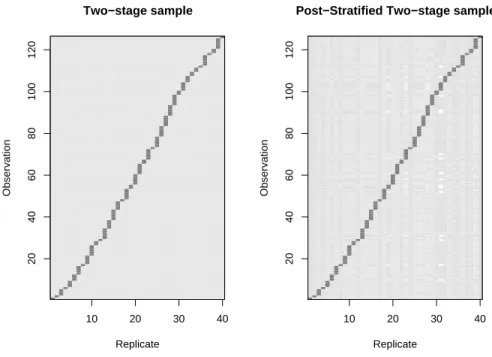
The full set of replicate weights can be displayed with the image function, and are given in Figure 1. The structure of JK1 weights can easily be seen in both images. On the right, the faint striping of the background indicates the
small adjustments in weights needed for post-stratification. The adjustments are largest in replicate number 31, which corresponds to a school district where all the sampled schools were high schools.
10 20 30 40 20 40 60 80 100 120 Replicate Observation Two−stage sample 10 20 30 40 20 40 60 80 100 120 Replicate Observation
Post−Stratified Two−stage sample
Figure 1: Replicate weights for two-stage cluster sample with and without post-stratification.
Finally, to illustrate raking we consider the proportion of schools that met their school-wide growth target in the API program
> rclus2r<-rake(rclus2, list(~stype, ~sch.wide),
+ list(pop.types, xtabs(~sch.wide,data=apipop)))
As these two variables are far from independent in the population, there is some efficiency gain but not as much as if the population joint distribution of the two variables were used for post-stratification.
> popboth<-xtabs(~stype+sch.wide,data=pop) > popboth sch.wide stype No Yes E 472 3949 H 334 421 M 266 752
> svrepmean(~api00, rclus2) mean SE api00 703.81 23.402 > svrepmean(~api00, rclus2p) mean SE api00 708.57 21.865 > svrepmean(~api00, rclus2r) mean SE api00 710.51 21.351 > svrepmean(~api00, rclus2p2) mean SE api00 710.54 20.587
5.2
Design specified only by replicates
In the example above we created replicate weights for a survey whose sampling design was known. The package can also be used to analyse data where replicate weights are supplied and the design is otherwise unspecified.
As an example, consider the Alcohol and Drug Services Study (ADSS) con-ducted for the Substance Abuse and Mental Health Services Administration. Data for this study are available from the Inter-University Consortium for Polit-ical and Social Research (http://www.icpsr.umich.edu/), as are descriptions of the design and analysis conducted by Westat (Mohadjeret al, 2000). This is a multistage survey of facilities providing treatment for substance abuse. The data file contains 2394 records and 991 variables. In this example we look at Phase I of the study, which involves stratified sampling of facilities. Phases II and III involve further subsampling of clients.
The data files contain 200 replicate weights that are based on a stratified jackknife (JKn) with modifications to reduce very large weights, account for nonresponse, and for other reasons. Separate files contain the finite population correction factors and the quantity we have calledci orrscales.
The design is specified by:
adss<-svrepdesign(data = adssdata, repweights = adssdata[, 782:981], scale = 1, rscales = adssjack, type = "other",
weights = ~PH1FW0, combined.weights = TRUE, fpc=adssfpc, fpctype="correction")
whereadssdatais the data frame containing all the survey data, andadssjack andadssfpcare the stratified jackknifeci and the finite population correction
factors. Thecombined.weightsoption indicates that the replicate weights al-ready incorporate the original sampling probabilities.
An example is given in the ADSS User’s Manual (Westat, 2000) of computing the mean number of clients (B1J2) for each facility type (TYPCARE5). This could be done with a linear regression
summary(model1) Call:
svrepglm(formula = B1J2 ~ factor(TYPCARE5) - 1, design = adss) Survey design:
svrepdesign(data = adssdata, repweights = adssdata[, 782:981],
scale = 1, rscales = adssjack, type = "other", weights = ~PH1FW0, combined.weights = TRUE, fpc = adssfpc, fpctype = "correction") Coefficients:
Estimate Std. Error t value Pr(>|t|) factor(TYPCARE5)1 14.6843 0.9901 14.83 <2e-16 *** factor(TYPCARE5)2 27.5658 1.3572 20.31 <2e-16 *** factor(TYPCARE5)3 250.3610 8.5202 29.38 <2e-16 *** factor(TYPCARE5)4 92.0009 3.6443 25.25 <2e-16 *** factor(TYPCARE5)5 114.1075 10.1071 11.29 <2e-16 *** ---Signif. codes: 0 ‘***’ 0.001 ‘**’ 0.01 ‘*’ 0.05 ‘.’ 0.1 ‘ ’ 1 This example illustrates the relationship betweeen memory and speed for the survey package. It takes 5–6 seconds to run on a PC with 1Gb of memory, and 15 seconds on an Apple Powerbook with only 256Mb. Peak memory usage is about 290Mb. It is interesting to compare this with the estimate given by Dippoet al (1984) for CPU time on an IBM 370 mainframe running the early
NASSVAR replicate-weights program. Their estimate for this analysis would be 54 CPU-seconds: twenty years advance in computing permits us to use an interpreted language on commodity hardware and still run nearly ten times faster.
5.3
Comparisons with other packages
Thesurveypackage provides much, but not all, of the survey analysis function-ality of SUDAAN or of Stata with the add-onsurvwgtcode of Winter (2002). The most important exceptions are tests for association in contingency tables. Most other software will compute variances either by Taylor linearisation or from replicates, but not both.
Other differences result from the underlying properties of R. The survey package is slow and requires a lot of memory to analyse large surveys, espe-cially under Windows. It is harder to learn than menu-driven programs such as WesVar, but on the other hand is more flexible and easier to extend.
Despite the similarity of R and S-PLUS, thesurveypackage would require some editing to be used with S-PLUS. The fileporting.to.Sgives suggestions and the LGPL license of the code is intended to remove any concerns about the use of the code on other systems.
5.4
Acknowledgements
This paper and software has been considerably improved by the comments of users and of the editors and reviews.
6
References
Bellhouse, D. R. (1985), Computing methods for variance estimation in complex surveys. Journal of Official Statistics, 1 , 323-329
Binder, D. A. (1983) On the Variances of Asymptotically Normal Estimators from Complex Surveys. International Statistical Review 51: 279–292.
Brick, J. M., Morganstein, D., Valliant, R. (2000)Analysis of complex sur-vey data using replication Westat: Rockville, MD. http://www.westat.com/ wesvar/techpapers/ACS-Replication.pdf
Cochran, W.S. (1977)Sampling Techniques(3rd edition). New York: Wiley. Dippo, C. S., Fay, R. E., Morganstein, D. (1984) Computing variances from samples with replicate weights. Proceedings of the ASA Section on Survey
Re-search Methods1984, 489–494http://www.amstat.org/sections/srms/Proceedings/ papers/1984_094.pdf
DuMouchel, W. H., Duncan, G. J. (1983) Using Sample Survey Weights in Multiple Regression Analyses of Stratified SamplesJournal of the American Statistical Association 78: 535-543.
Judkins, D. R. (1990) Fay’s method for variance estimation. Journal of Official Statistics 6: 223–239.
Levy P.S., Lemeshow S (1999) Sampling of Populations: Methods and Ap-plications (3rd edition). New York, NY: Wiley.
Mohadjer, L., Yansaneh, I., Krenzke, T., Dohrmann, S. (2000)Sample De-sign, Selection, and Estimation for Phase I of ADSS. Westat: Rockville, MD. http://www.samhsa.gov/oas/ADSS/SampleDesign1.pdf
Plackett, R. L., Burman, J. P. (1946) The design of optimum multifactorial experiments. Biometrika 33, 305-325.
Shao J., Tu D. (1995)The Jackknife and Bootstrap. New York, NY: Springer. Westat (2000) Alcohol and Drug Services Study (ADSS). Data file user’s manual for the ADSS Phase I facility interview file http://www.samhsa.gov/ oas/ADSS/ADSS1FacilityCB.pdf.
Winter, N. (2002)SURVWGT: Stata module to create and manipulate survey weights. http://econpapers.hhs.se/software/bocbocode/s427503.htm
Wolter, K. M. (1985) Introduction to Variance Estimation. New York, NY:Springer.