ON RANDOM ITERATED FUNCTION SYSTEMS WITH GREYSCALE
MAPS
MATTHEW
DEMERS
1,HERB
KUNZE
B
,
2 ANDDAVIDE
LA
TORRE
31University of Guelph, Department of Mathematics & Statistics, Guelph, Ontario, Canada;2University of
Guelph, Department of Mathematics & Statistics, Guelph, Ontario, Canada;3University of Milan, Department
of Economics, Business and Statistics, Milan, Italy
e-mail: [email protected]; [email protected]; [email protected]
(Received January 18, 2012; revised April 27, 2012; accepted May 8, 2012)
ABSTRACT
In the theory of Iterated Function Systems (IFSs) it is known that one can find an IFS with greyscale maps (IFSM) to approximate any target signal or image with arbitrary precision, and a systematic approach for doing so was described. In this paper, we extend these ideas to the framework of random IFSM operators. We consider the situation where one has many noisy observations of a particular target signal and show that the greyscale map parameters for each individual observation inherit the noise distribution of the observation. We provide illustrative examples.
Keywords: random fixed point equations, random iterated function systems, collage theorem.
INTRODUCTION
In fractal imaging compression and coding based on Generalized Fractal Transforms (GFT), one seeks to approximate a target image or signal by the fixed points of a contractive fractal transform operator. The usual formulation involves a fixed set of geometric contraction maps along with a corresponding set of greyscale adjustment maps. The inverse problem requires one to find the best greyscale map parameters for a given target image. The solution process is referred to as “collage coding” because of the visual effect of the contraction maps; it applies the collage theorem, a simple consequence of Banach’s fixed point theorem. The approximation of the target image or signal can be generated through iteration of the fractal
transform (see Hutchinson, 1981; Barnsleyet al.,
1985; Barnsley and Demko, 1985; Barnsley, 1989; Barnsley and Hurd, 1993; Forte and Vrscay, 1995; 1999;Iacus and La Torre,2005b;a;Kunzeet al.,2008; La Torreet al., 2009; La Torre and Vrscay, 2011 for more details and applications).
In Forte and Vrscay (1995), the authors showed that one can find an iterated function system with greyscale maps (IFSM) to approximate any target signal or image with arbitrary precision, and they provided a suboptimal but systematic approach for doing so.
The goal of this paper is to extend the work in Forte and Vrscay(1995) to the framework of random IFSM operators. We consider the situation where one has many noisy observations of a particular target signal and show that the greyscale map parameters
for each individual observation inherit the noise distribution of the observation.
Prior to these results, we present several
short background sections. First, we discuss the deterministic collage coding framework and quickly summarize the related IFSM setting. Then we present the random collage coding framework. Finally, we formulate the random IFSM operator framework and present some illustrative numerical examples.
FIXED POINT EQUATIONS AND
COLLAGE THEOREM
In this section, we present some basic contraction map results that will be used in later sections. Let (X,dX)denote a complete metric space. ThenT :X→
X is contractive if there exists ac∈[0,1)such that
dX(T x,Ty)≤cdX(x,y) for all x,y∈X. (1)
We normally refer to the infimum of all c values
satisfying Eq.1as thecontraction factorofT.
Theorem 1 (Banach): Let (X,dX) be a complete
metric space. Also let T :X → X be a contraction mapping with contraction factor c∈[0,1). Then there exists a uniquex¯∈X such thatx¯=Tx. Moreover, for¯ any x∈X , dX(Tnx,x¯)→0as n→∞.
Theorem 2 (Continuity theorem for fixed points, Centore and Vrscay,1994): Let(X,dX)be a complete
with contraction factors c1 and c2and fixed pointsy¯1 andy¯2, respectively. Then
dX(y¯1,y¯2)≤
1 1−min{c1,c2}
dX,sup(T1,T2) (2)
where
dX,sup(T1,T2) =sup
x∈X
dX(T1(x),T2(x)). (3)
Banach’s fixed point theorem provides a mechanism to
solve theforward problem of the fixed point equation
x=T x: Given a contraction T, construct, or at least
approximate, its fixed point ¯x. And the continuity
theorem establishes that small changes in a contraction mapping produce small changes in the associated fixed points.
A formal mathematicalinverse problemassociated
with the fixed point equationx=T xis: Given a target element xand anε >0, find a contraction map T(ε) (perhaps from a suitable family of operators) with fixed point ¯x(ε)such thatd(x,x¯(ε))<ε. In the case that one is able to solve such an inverse problem to arbitrary precision, i.e.,ε →0, then one may identify the target xas the fixed point of a contractive operatorT onX.
In practical applications, however, it is not generally possible to find such solutions to arbitrary accuracy nor is it even feasible to search for such contraction maps. Instead, one makes use of the following result, which is a simple consequence of Banach’s fixed point theorem.
Theorem 3 (“Collage theorem”, Barnsley et al., 1985): Let (X,d) be a complete metric space and T :X → X a contraction mapping with contraction factor c∈[0,1). Then for any x∈X ,
d(x,x¯)≤ 1
1−cd(x,T x), (4)
wherex is the fixed point of T .¯
The approximation error d(x,x¯) is bounded above
by the so-called collage distance d(x,T x). Most
practical methods of solving such inverse problems,
for example, fractal image coding (Fisher, 1995; Lu,
2003), search for an operatorT for which the collage distance is as small as possible, while ensuring that
c is sufficiently far away from one. In other words,
these methods seek an operatorT that maps the target
x as close as possible to itself. This inverse problem
solution procedure, often referred to ascollage coding, is most often performed by considering a parametrized
family of contraction mapsTλ,λ ∈Λ⊂Rn, and then
minimizing the collage distanced(x,Tλx).
Finally, we mention another interesting result which is a simple consequence of Banach’s fixed point theorem.
Theorem 4 (“Anti-collage theorem”,Vrscay and Saupe, 1999): Let (X,d) be a complete metric space and T :X → X a contraction mapping with contraction factor c∈[0,1). Then for any x∈X ,
d(x,x¯)≥ 1
1+cd(x,T x), (5)
wherex is the fixed point of T .¯
FORMAL SOLUTION TO THE
INVERSE PROBLEM FOR
ITERATED FUNCTION SYSTEMS
WITH GREYSCALE MAPS
The method of iterated function systems with greyscale maps (IFSM), as formulated by Forte and Vrscay (1995), can be used to approximate a given elementuofL2([0,1]). We consider the case in which u:[0,1]→[0,1]and the space
X=©
u:[0,1]→[0,1],u∈L2[0,1]ª
. (6)
The ingredients of an N-map IFSM on X are
(Forte and Vrscay,1995;1999)
1. a set of N contractive mappings w =
{w1,w2, . . . ,wN}, wi : [0,1] → [0,1], satisfying
the covering conditionSN
i=1wi([0,1]) = [0,1], and
most often affine in form:
wi(x) =six+ai, 0≤si<1, i=1,2, . . . ,N;
(7)
2. a set of associated functions – the greyscale maps –
φ ={φ1,φ2, . . . ,φN},φi :R→R. Affine maps are
usually employed:
φi(t) =αit+βi, (8)
with the conditions
αi,βi∈[0,1] (9)
and
0≤
N
∑
i=1
Associated with theN-map IFSM(w,φ)is thefractal transformoperatorT, the action of which on a function
u∈X is given by
(Tu)(x) =
N
∑
i=1 ′φ
i(u(w−i 1(x))), (11)
where the prime means that the sum operates on all those terms for whichw−i 1is defined.
Theorem 5 (Forte and Vrscay,1995): T :X→X and for any u,v∈X we have
d2(Tu,T v)≤Cd2(u,v) (12)
where
C=
N
∑
i=1 s
1 2
i αi. (13)
When C <1, then T is contractive on X, implying
the existence of a unique fixed point ¯u∈X such that
¯ u=Tu¯.
The squared collage distance function associated
with an N-map IFSM may be written as a quadratic
form,
∆2=zTAz+bTz+c, (14) where z = (α1, . . .αk,β1, . . . ,βk). We observe that in
the special that the setswi([0,1]),i=1, . . . ,N, are
non-overlapping, for each i the values of αi and βi that
minimize∆2 can be determined by solving a separate
minimization problem using least squares.
The inverse problem associated with IFSM can, in principle, be solved to arbitrary accuracy, using
a procedure defined in Forte and Vrscay (1995). The
maps wk are chosen from an infinite setW of fixed
affine contraction maps on [0,1] which satisfy the
following properties.
Definition 1 We say that W generates an m-dense and nonoverlapping family A of subsets of I if for every ε>0and every B⊂I there exists a finite set of integers ik, ik≥1,1≤k≤N, such that
(i) A=∪N
k=1wik(I)⊂B, (ii) m(B\A)<ε, and
(iii) m(wik(I)∩wil(I)) =0if k6=l, where m denotes Lebesgue measure.
Let
WN={w1, . . .wN} (15)
be the N truncations of w. Let ΦN = {φ
1, . . . ,φN}
be theN-vector of affine grey level maps. Let zN be
the solution of the previous quadratic optimization
problem and ∆2
N,min = ∆2N(zN). In Forte and Vrscay
(1995), the following result was proved.
Theorem 6
∆2N,min→0as N→∞.
Using the Collage Theorem, the inverse problem may be solved to arbitrary accuracy. A practical choice for
the contraction mapswonX= [0,1]is
wi j(x) =2−i(x+j−1),i=1,2, . . . , j=1,2, . . . ,2i.
RANDOM FIXED POINT
EQUATIONS
Let (Ω,F,P) denote a probability space and
(X,d) a metric space. A mapping T :Ω×X →X is
called arandom operatorif for anyx∈X the function
T(.,x)is measurable. A measurable mappingx:Ω→
X is called arandom fixed pointof a random operator
T ifxis a solution of the equation
T(w,x(w)) =x(w). (16)
for a.e. ω ∈ Ω. A random operator T is called
continuous (Lipschitz, contraction) if for a.e. w ∈
Ω we have that T(w, .) is continuous (Lipschitz,
contraction). There are many papers in the literature that deal with such equations for single-valued and
set-valued random operators (see Bharucha-Reid, 1972;
Itoh,1979;Papageorgiou,1988;Lin,1995;Liu,1997; Shahzad, 2001; 2004a;b). Solutions of random fixed point equations and inclusions are usually produced by means of stochastic generalizations of classical fixed point theory.
Let (Ω,F,P) be a probability space and let
(X,dX)be a complete metric space. LetT:Ω×X→X
be a given operator. We look for the solution of the equation
T(ω,x(ω)) =x(ω) (17)
for a.e. ω ∈ Ω\A and P(A) = 0. Suppose that the
operatorT satisfies the inequality
d(T(ω,x),T(ω,y))≤c(ω)d(x,y), (18)
where c(ω):Ω→X. WhenT satisfies this property,
we say thatT is ac(ω)-Lipschitz operator. If c(ω)≤ c<1 a.e., with ω ∈Ω\AandP(A) =0 then we say
that T is a c(ω)-contraction. In this case for ω ∈
Ω\A there exists a unique pointx(ω)∈X. It is clear that the uniqueness makes sense except for sets of measure zero. Once again, the inverse problem can be
formulated as: Given a functionx:Ω→Xand a family
of operatorsTλ :Ω×X→X, findλ such thatxis the
solution of random fixed point equation
Tλ(ω,x(ω)) =x(ω). (19)
Corollary 1 (“Regularity conditions”): Let(Ω,F,P)
be a probability space and (X,dX) be a
complete metric space. Let T : Ω×X → X be a given c(ω)-contraction. Then dX(x(ω1),x(ω2)) ≤
1 1−csup
x∈X
d(T(ω1,x),T(ω2,x))
Corollary 2 (“Continuity Theorem”): Let (Ω,F,P)
be a probability space and let (X,dX) be a complete
metric space. Let T1:Ω×X→X and T2:Ω×X →X be c1(ω)- and c2(ω)-contractions respectively. Then
dX(x1(ω),x2(ω))≤
1 1−min{c1,c2}
sup
x∈X
dX(T1(ω,x),T2(ω,x)).
Theorem 7 (“Collage Theorem”): Let(Ω,F,P)be a
probability space and let(X,dX)be a complete metric
space. Let T :Ω×X→X be a given c(ω)-contraction. Then
1
1+cdX(x(ω),T(ω,x(ω)))≤dX(x(ω),x¯(ω))≤ 1
1−cdX(x(ω),T(ω,x(ω))),
a.e.ω∈Ω, wherex¯(ω)is the solution of T(ω,x¯(ω)) = ¯
x(ω).
The above described approach to deal with random fixed point equations does not guarantee, in general,
the measurability of the function x : Ω → X with
respect to the sigma algebraF. In order to overcome
this difficulty, we provide an abstract formulation of the same problem which guarantees the measurability ofx.
Recall that(X,d)is said to be a Polish space if it is a separable complete metric space. In random fixed point theory, separability plays an important role. Two important examples of Polish metric spaces which will be useful in the following areC([a,b]) andL2([a,b]).
Consider now the spaceY of all measurable functions
x :Ω→ X. If we define the operator ˜T :Y →Y as
(T y˜ )(ω) =T(ω,x(ω))the solutions of this fixed point
equation on Y are the solutions of the random fixed
point equation T(ω,x(ω)) =x(ω). Suppose that the metric dX is bounded, that is dX(x1,x2)≤K for all x1,x2∈X. So the functionψ(ω) =dX(x1(ω),x2(ω)):
Ω→Ris an element ofL1(Ω) for allx1,x2∈Ω. We
can then define on the spaceY the following function
dY(x1,x2) = Z
ΩdX(x1(ω),x2(ω))dω. (20)
It can be shown that the space (Y,dY) is a complete
metric space. The following result holds.
Theorem 8 (Itoh,1977): Let X be a Polish space, and T:Ω×X→X be a mapping such that for eachω∈Ω the function T(ω, .)is c(ω)-Lipschitz and for each x∈ X the function T(.,x)is measurable. Let x:Ω→X be a measurable mapping; then the mappingξ :Ω→X defined byξ(ω) =T(ω,x(ω))is measurable.
The previous theorem (Eq.8) holds if T(ω,·) is only
continuous (see, for instance,Himmelberg,1975).
Corollary 3 Let X be a Polish space and T:Ω×X→ X be a mapping such that for eachω∈Ωthe function T(ω,·) is a c(ω)-contraction. Suppose that for each x∈X the function T(·,x) is measurable. Then there exists a unique solution of the equationT˜x¯=x that is¯ T(ω,x¯(ω)) =x¯(ω)for a.e.ω ∈Ω.
In these results separability plays a crucial role. In fact
using this hypothesis and Theorem 8 one can prove
that the function ξ(ω) =T(ω,x(ω)) is measurable,
that is ˜T :Y →Y. Other random fixed point theorems
for contraction mappings in Polish spaces can be found inSpaˇcek(1955);Hanˇs(1957);Bharucha-Reid(1972). The inverse problem can be formulated as: Given a function ¯x:Ω→Xand a family of operators ˜Tλ:Y→
Y find λ such that ¯x is the solution of random fixed
point equation
˜
Tλx¯=x¯, (21)
that is,
Tλ(ω,x¯(ω)) =x¯(ω). (22)
Now, with the collage and continuity theorems, we may state the following.
Corollary 4 Let X be a Polish space and T:Ω×X→ X be a mapping such that for eachω∈Ωthe function T(ω,·) is a c(ω)-contraction. Suppose that for each x∈X the function T(·,x)is measurable. Then for any x∈Y ,
1
1+cdY(x,T x˜ )≤dY(x,x¯)≤ 1
1−cdY(x,T x˜ ), (23)
FORMAL SOLUTION TO THE
INVERSE PROBLEM FOR
RANDOM ITERATED FUNCTION
SYSTEMS WITH GREYSCALE
MAPS
We now formulate a Random IFSM fractal
transform that is analogous to the deterministic fractal
transform in Eq.11.
Let(Ω,F,P)be a probability space and consider
now the following operatorT :X×Ω→Xdefined by
T(ω,u) = (Tu)(x)
=
N
∑
i=1 ′α
i(u(w−i 1(x))) +βi(ω)
= (T∗u) +β(ω),
where β(ω) =∑Ni=1′βi(ω). That is, we suppose that
the greyscale maps take the form
φi(ω,t) =αit+βi(ω), (24)
where βi are random variables with mean µi and
|βi(ω)|<δ a.e.ω ∈Ω, and that
αi,δ ∈[0,1] (25)
with
0≤
N
∑
i=1
(αi+δ)<1. (26)
We randomize only the βi parameters since the
randomness in the other term ofT(ω,u)is transmitted by the functionu. Let
Y={u:Ω→X,uis measurable} (27)
and consider the function
ψ(ω):=dX(u1(ω),u2(ω)) =ku1(ω)−u2(ω)k2.
From the hypotheses it is clear thatψ(ω)∈L1(Ω). We know that(Y,dY)is a complete metric space where
dY(u1,u2) = Z
Ωku1(ω)−u2(ω)k2dω . (28)
Obviously, the function ξ(ω) := (T∗u)(ω) +β(ω)
belongs toY becauseT∗is Lipschitz onXand theβ is
measurable. If we define ˜T :Y →Y where ˜T u=ξ we
have
dY(T u˜ 1,T u˜ 2) = Z
Ωk(T
∗u1)(ω) +β(ω)−(T∗u2)(ω)−β(ω)k 2dω=
Z
Ω
ku1(ω)−u2(ω)k2dω =CdY(u1,u2).
So there exists ¯u∈Y such that ˜Tu¯=u¯, that is, ¯u(ω) = T(ω,u¯(ω))for a.e.ω∈Ω. That is,
¯
u(ω,x) = (T∗u¯(ω))(x) +β(ω)
=
N
∑
i=1 ′α
i(u¯(ω,wi−1(x))) +βi(ω) (29)
for a.e. x ∈ [0,1]. The inverse problem of finding
the random variables βi(ω), perhaps to arbitrary
accuracy, is note possible given the random nature of the problem. Instead, we suppose that the function
¯
u(ω,x):Ω×[0,1]→Ris integrable and let
¯ u(x) =
Z
Ω[u¯(ω)](x)dω =
Z
Ωu¯(ω,x)dω. (30)
Thus Eq.29becomes
¯ u(x) =
N
∑
i=1 ′α
i(u¯(w−i 1(x))) +µi. (31)
That is, the expectation value of ¯u(ω,x)is the solution
of a deterministic N-map IFSM on X (cf. Eq. 11).
We observe in Eq. 31 another motivation for not
randomizing the parametersαi: the expectation of the
productαiu(·)becomes complicated.
Suppose that we have N observations, u(ω1),
u(ω2), . . ., u(ωn), of the variable u(ω). Choose a set
of greyscale maps, as in Eq. 15. We collage code
each observation,u(ωk),k=1, . . . ,n, to find the set of
minimal collage parameters αik and βik,k =1, . . . ,n,
i = 1, . . . ,N. As a result of our earlier discussion, if the observations differ only by a uniform additive noise factor, we expect that the distribution of the βik
parameters, k=1. . . ,n will inherit that distribution, with meanµi.
NUMERICAL EXAMPLES
This section provides several numerical examples which illustrate the above formulation and “mean property.”
Example:We define the IFS maps
wi j(x) =2−i(x+j−1), i=1, . . . ,4, j=1,2, . . . ,2i,
with associated greyscale maps φi j(t) =αi jt+βi j. In
this example, we consider the target function
u(x) =0.8x2+0.1. (32)
We constructNobservations of the function by adding
constant noise to it:
uk(x) =u(x) +νk, k=1, . . . ,N,
where |νk| < 0.1 with mean zero. The picture in
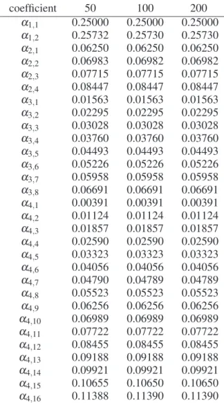
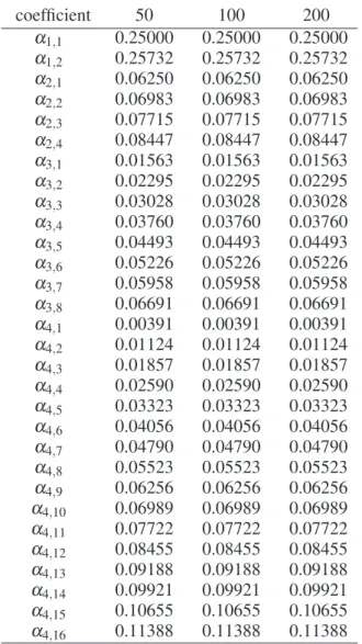
Table 1. Greyscale map mean parameters αi,j in the
case of constant additive noise.
coefficient 50 100 200
α1,1 0.25000 0.25000 0.25000
α1,2 0.25732 0.25730 0.25730
α2,1 0.06250 0.06250 0.06250
α2,2 0.06983 0.06982 0.06982
α2,3 0.07715 0.07715 0.07715
α2,4 0.08447 0.08447 0.08447
α3,1 0.01563 0.01563 0.01563
α3,2 0.02295 0.02295 0.02295
α3,3 0.03028 0.03028 0.03028
α3,4 0.03760 0.03760 0.03760
α3,5 0.04493 0.04493 0.04493
α3,6 0.05226 0.05226 0.05226
α3,7 0.05958 0.05958 0.05958
α3,8 0.06691 0.06691 0.06691
α4,1 0.00391 0.00391 0.00391
α4,2 0.01124 0.01124 0.01124
α4,3 0.01857 0.01857 0.01857
α4,4 0.02590 0.02590 0.02590
α4,5 0.03323 0.03323 0.03323
α4,6 0.04056 0.04056 0.04056
α4,7 0.04790 0.04789 0.04789
α4,8 0.05523 0.05523 0.05523
α4,9 0.06256 0.06256 0.06256
α4,10 0.06989 0.06989 0.06989
α4,11 0.07722 0.07722 0.07722
α4,12 0.08455 0.08455 0.08455
α4,13 0.09188 0.09188 0.09188
α4,14 0.09921 0.09921 0.09921
α4,15 0.10655 0.10650 0.10650
α4,16 0.11388 0.11390 0.11390
Fig. 1.Ten realizations for constant additive noise and place-dependent additive noise.
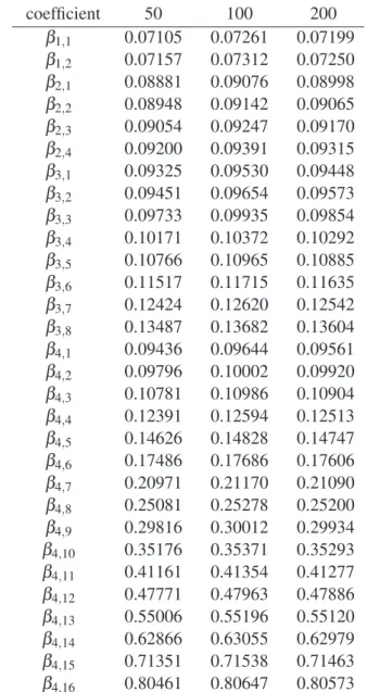
Tables 1 and 2 presents the mean value of
each greyscale map parameter obtained by collage coding the separate realizations. The calculations were performed for 50, 100, and 200 realizations, using Maple.
Table 2. Greyscale map mean parameters βi,j in the
case of constant additive noise.
coefficient 50 100 200
β1,1 0.07105 0.07261 0.07199
β1,2 0.07157 0.07312 0.07250
β2,1 0.08881 0.09077 0.08998
β2,2 0.08948 0.09142 0.09065
β2,3 0.09054 0.09247 0.09170
β2,4 0.09200 0.09391 0.09315
β3,1 0.09325 0.09530 0.09448
β3,2 0.09451 0.09655 0.09573
β3,3 0.09733 0.09935 0.09854
β3,4 0.10171 0.10372 0.10292
β3,5 0.10766 0.10965 0.10885
β3,6 0.11517 0.11715 0.11635
β3,7 0.12424 0.12620 0.12542
β3,8 0.13487 0.13682 0.13604
β4,1 0.09436 0.09644 0.09561
β4,2 0.09796 0.10002 0.09920
β4,3 0.10781 0.10986 0.10904
β4,4 0.12391 0.12594 0.12513
β4,5 0.14626 0.14828 0.14747
β4,6 0.17486 0.17686 0.17606
β4,7 0.20971 0.21170 0.21090
β4,8 0.25081 0.25278 0.25200
β4,9 0.29816 0.30012 0.29934
β4,10 0.35176 0.35371 0.35293
β4,11 0.41161 0.41354 0.41277
β4,12 0.47771 0.47963 0.47886
β4,13 0.55006 0.55196 0.55120
β4,14 0.62866 0.63055 0.62979
β4,15 0.71351 0.71538 0.71463
β4,16 0.80461 0.80647 0.80573
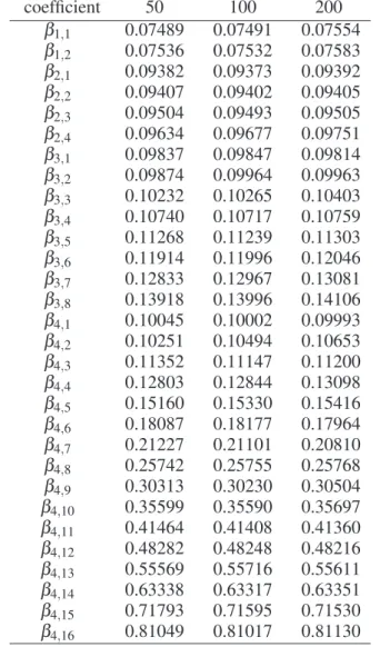
Tables 3 and 4 present the greyscale parameters
obtained upon collage coding the mean observation
u∗(x) = 1 N
N
∑
k=1 uk(x).
We see that the corresponding values in the tables agree increasingly well as the number of realizations
increase. In all cases, for any fixed choices of i and
j, the value ofαi,j is the same across all simulations
and across the two tables. In fractal imaging, the α
parameters represent a contrast adjustment and theβ
parameters represent a brightness adjustment. In this example, the different realizations differ only by a vertical shift, so the corresponding fractal codes differ only in the brightness parameters. We also observe that values in the tables agree to at least two decimal places
with the IFSM parameters for the unnoised signal,
Table 3.Greyscale map parametersαi,j for the mean
observation in the case of constant additive noise.
coefficient 50 100 200
α1,1 0.25000 0.25000 0.25000
α1,2 0.25730 0.25730 0.25730
α2,1 0.06250 0.06250 0.06250
α2,2 0.06982 0.06982 0.06982
α2,3 0.07715 0.07715 0.07715
α2,4 0.08447 0.08447 0.08447
α3,1 0.01562 0.01562 0.01562
α3,2 0.02295 0.02295 0.02295
α3,3 0.03028 0.03028 0.03028
α3,4 0.03760 0.03760 0.03760
α3,5 0.04493 0.04493 0.04493
α3,6 0.05226 0.05226 0.05226
α3,7 0.05958 0.05958 0.05958
α3,8 0.06691 0.06691 0.06691
α4,1 0.00391 0.00391 0.00391
α4,2 0.01124 0.01124 0.01124
α4,3 0.01857 0.01857 0.01857
α4,4 0.02590 0.02590 0.02590
α4,5 0.03323 0.03323 0.03323
α4,6 0.04056 0.04056 0.04056
α4,7 0.04789 0.04789 0.04789
α4,8 0.05523 0.05523 0.05523
α4,9 0.06256 0.06256 0.06256
α4,10 0.06989 0.06989 0.06989
α4,11 0.07722 0.07722 0.07722
α4,12 0.08455 0.08455 0.08455
α4,13 0.09188 0.09188 0.09188
α4,14 0.09921 0.09921 0.09921
α4,15 0.10650 0.10650 0.10650
α4,16 0.11390 0.11390 0.11390
Table 4. Greyscale map parametersβi,j for the mean
observation in the case of constant additive noise.
coefficient 50 100 200
β1,1 0.07105 0.07261 0.07199
β1,2 0.07157 0.07312 0.07250
β2,1 0.08881 0.09076 0.08998
β2,2 0.08948 0.09142 0.09065
β2,3 0.09054 0.09247 0.09170
β2,4 0.09200 0.09391 0.09315
β3,1 0.09325 0.09530 0.09448
β3,2 0.09451 0.09654 0.09573
β3,3 0.09733 0.09935 0.09854
β3,4 0.10171 0.10372 0.10292
β3,5 0.10766 0.10965 0.10885
β3,6 0.11517 0.11715 0.11635
β3,7 0.12424 0.12620 0.12542
β3,8 0.13487 0.13682 0.13604
β4,1 0.09436 0.09644 0.09561
β4,2 0.09796 0.10002 0.09920
β4,3 0.10781 0.10986 0.10904
β4,4 0.12391 0.12594 0.12513
β4,5 0.14626 0.14828 0.14747
β4,6 0.17486 0.17686 0.17606
β4,7 0.20971 0.21170 0.21090
β4,8 0.25081 0.25278 0.25200
β4,9 0.29816 0.30012 0.29934
β4,10 0.35176 0.35371 0.35293
β4,11 0.41161 0.41354 0.41277
β4,12 0.47771 0.47963 0.47886
β4,13 0.55006 0.55196 0.55120
β4,14 0.62866 0.63055 0.62979
β4,15 0.71351 0.71538 0.71463
β4,16 0.80461 0.80647 0.80573
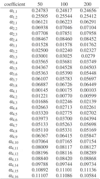
Example: We repeat the preceding example, this
time adding place-dependent noise to produce the N
realizations:
uk(x) =u(x) +νk(x), k=1, . . . ,N,
whereu(x) =0.8x2+0.1, as before,|νk(x)|<0.1 for
allx, and, for each fixedx,νk(x)are samples from the
re-scaled distribution N(0,0.01). The right picture
in Fig. 1 presents ten realizations. The results are
Table 5. Greyscale map mean parameters αi,j in the
case of place-dependent additive noise with a normal distribution.
coefficient 50 100 200
α1,1 0.24783 0.24817 0.24656
α1,2 0.25505 0.25544 0.25412
α2,1 0.06121 0.06223 0.06291
α2,2 0.06938 0.07046 0.07104
α2,3 0.07708 0.07851 0.07958
α2,4 0.08467 0.08460 0.08452
α3,1 0.01528 0.01578 0.01762
α3,2 0.02500 0.02240 0.02327
α3,3 0.03001 0.03025 0.0279
α3,4 0.03565 0.03681 0.03749
α3,5 0.04367 0.04528 0.04503
α3,6 0.05363 0.05390 0.05448
α3,7 0.06107 0.05783 0.05697
α3,8 0.06887 0.06726 0.06449
α4,1 0.00145 0.00175 0.00103
α4,2 0.01221 0.00770 0.00599
α4,3 0.01686 0.02246 0.02139
α4,4 0.02663 0.02713 0.02261
α4,5 0.03320 0.02775 0.02702
α4,6 0.03973 0.03700 0.04394
α4,7 0.05133 0.05263 0.05698
α4,8 0.05110 0.05331 0.05169
α4,9 0.06367 0.06415 0.05847
α4,10 0.07064 0.07165 0.07154
α4,11 0.08009 0.08117 0.08127
α4,12 0.08196 0.08116 0.08289
α4,13 0.08840 0.08420 0.08868
α4,14 0.09788 0.09744 0.09734
α4,15 0.10892 0.11101 0.11136
α4,16 0.11107 0.11086 0.10584
Table 6. Greyscale map mean parameters βi,j in the
case of place-dependent additive noise with a normal distribution.
coefficient 50 100 200
β1,1 0.07567 0.07569 0.07636
β1,2 0.07616 0.07611 0.07662
β2,1 0.09393 0.09383 0.09400
β2,2 0.09424 0.09417 0.09423
β2,3 0.09511 0.09500 0.09509
β2,4 0.09649 0.09693 0.09764
β3,1 0.09838 0.09843 0.09808
β3,2 0.09875 0.09962 0.09961
β3,3 0.10234 0.10268 0.10412
β3,4 0.10740 0.10717 0.10756
β3,5 0.11273 0.11245 0.11306
β3,6 0.11915 0.11994 0.12040
β3,7 0.12841 0.12973 0.13083
β3,8 0.13923 0.14004 0.14117
β4,1 0.10043 0.09999 0.09986
β4,2 0.10254 0.10497 0.10664
β4,3 0.11348 0.11149 0.11200
β4,4 0.12806 0.12842 0.13100
β4,5 0.15160 0.15332 0.15423
β4,6 0.18088 0.18174 0.17955
β4,7 0.21230 0.21107 0.20814
β4,8 0.25745 0.25764 0.25772
β4,9 0.30314 0.30231 0.30508
β4,10 0.35598 0.35589 0.35696
β4,11 0.41463 0.41407 0.41363
β4,12 0.48285 0.48257 0.48226
β4,13 0.55575 0.55723 0.55612
β4,14 0.63338 0.63320 0.63350
β4,15 0.71795 0.71599 0.71530
Table 7.Greyscale map parametersαi,j for the mean
observation in the case of place-dependent additive noise with a normal distribution.
coefficient 50 100 200
α1,1 0.24995 0.25030 0.24878
α1,2 0.25722 0.25759 0.25626
α2,1 0.06152 0.06250 0.06312
α2,2 0.06984 0.07086 0.07153
α2,3 0.07725 0.07870 0.07967
α2,4 0.08506 0.08504 0.08488
α3,1 0.01534 0.01568 0.01744
α3,2 0.02503 0.02235 0.02321
α3,3 0.03006 0.03031 0.02814
α3,4 0.03564 0.03679 0.03740
α3,5 0.04381 0.04543 0.04513
α3,6 0.05365 0.05386 0.05433
α3,7 0.06127 0.05801 0.05702
α3,8 0.06899 0.06750 0.06477
α4,1 0.00143 0.00178 0.00084
α4,2 0.01229 0.00781 0.00629
α4,3 0.01675 0.02249 0.02141
α4,4 0.02668 0.02705 0.02266
α4,5 0.03321 0.02780 0.02719
α4,6 0.03973 0.03692 0.04373
α4,7 0.05143 0.05280 0.05710
α4,8 0.05118 0.05356 0.05175
α4,9 0.06371 0.06419 0.05859
α4,10 0.07061 0.07159 0.07149
α4,11 0.08008 0.08115 0.08136
α4,12 0.08206 0.08141 0.08320
α4,13 0.08855 0.08437 0.08873
α4,14 0.09792 0.09758 0.09738
α4,15 0.10897 0.11110 0.11133
α4,16 0.11104 0.11083 0.10592
Table 8. Greyscale map parametersβi,j for the mean
observation in the case of place-dependent additive noise with a normal distribution.
coefficient 50 100 200
β1,1 0.07489 0.07491 0.07554
β1,2 0.07536 0.07532 0.07583
β2,1 0.09382 0.09373 0.09392
β2,2 0.09407 0.09402 0.09405
β2,3 0.09504 0.09493 0.09505
β2,4 0.09634 0.09677 0.09751
β3,1 0.09837 0.09847 0.09814
β3,2 0.09874 0.09964 0.09963
β3,3 0.10232 0.10265 0.10403
β3,4 0.10740 0.10717 0.10759
β3,5 0.11268 0.11239 0.11303
β3,6 0.11914 0.11996 0.12046
β3,7 0.12833 0.12967 0.13081
β3,8 0.13918 0.13996 0.14106
β4,1 0.10045 0.10002 0.09993
β4,2 0.10251 0.10494 0.10653
β4,3 0.11352 0.11147 0.11200
β4,4 0.12803 0.12844 0.13098
β4,5 0.15160 0.15330 0.15416
β4,6 0.18087 0.18177 0.17964
β4,7 0.21227 0.21101 0.20810
β4,8 0.25742 0.25755 0.25768
β4,9 0.30313 0.30230 0.30504
β4,10 0.35599 0.35590 0.35697
β4,11 0.41464 0.41408 0.41360
β4,12 0.48282 0.48248 0.48216
β4,13 0.55569 0.55716 0.55611
β4,14 0.63338 0.63317 0.63351
β4,15 0.71793 0.71595 0.71530
β4,16 0.81049 0.81017 0.81130
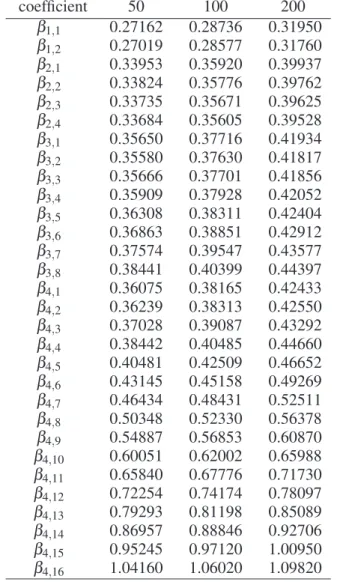
Example: We repeat the preceding example a last
time, with the place-dependent noise νk(x) being
samples from a beta distributionβ(1,2). The results
are presented in Tables 9–12, with the first table
presenting the means of the greyscale map parameters
Table 9. Greyscale map mean parameters αi,j in the
case of place-dependent additive noise with a beta distribution.
coefficient 50 100 200
α1,1 0.25000 0.25000 0.25000
α1,2 0.25732 0.25732 0.25732
α2,1 0.06250 0.06250 0.06250
α2,2 0.06983 0.06983 0.06983
α2,3 0.07715 0.07715 0.07715
α2,4 0.08447 0.08447 0.08447
α3,1 0.01563 0.01563 0.01563
α3,2 0.02295 0.02295 0.02295
α3,3 0.03028 0.03028 0.03028
α3,4 0.03760 0.03760 0.03760
α3,5 0.04493 0.04493 0.04493
α3,6 0.05226 0.05226 0.05226
α3,7 0.05958 0.05958 0.05958
α3,8 0.06691 0.06691 0.06691
α4,1 0.00391 0.00391 0.00391
α4,2 0.01124 0.01124 0.01124
α4,3 0.01857 0.01857 0.01857
α4,4 0.02590 0.02590 0.02590
α4,5 0.03323 0.03323 0.03323
α4,6 0.04056 0.04056 0.04056
α4,7 0.04790 0.04790 0.04790
α4,8 0.05523 0.05523 0.05523
α4,9 0.06256 0.06256 0.06256
α4,10 0.06989 0.06989 0.06989
α4,11 0.07722 0.07722 0.07722
α4,12 0.08455 0.08455 0.08455
α4,13 0.09188 0.09188 0.09188
α4,14 0.09921 0.09921 0.09921
α4,15 0.10655 0.10655 0.10655
α4,16 0.11388 0.11388 0.11388
Table 10.Greyscale map mean parametersβi,j in the
case of place-dependent additive noise with a beta distribution.
coefficient 50 100 200
β1,1 0.27162 0.28736 0.31950
β1,2 0.27019 0.28577 0.31760
β2,1 0.33953 0.35920 0.39937
β2,2 0.33824 0.35776 0.39762
β2,3 0.33735 0.35671 0.39625
β2,4 0.33684 0.35605 0.39528
β3,1 0.35650 0.37716 0.41934
β3,2 0.35580 0.37630 0.41817
β3,3 0.35666 0.37701 0.41856
β3,4 0.35909 0.37928 0.42052
β3,5 0.36308 0.38311 0.42404
β3,6 0.36863 0.38851 0.42912
β3,7 0.37574 0.39547 0.43577
β3,8 0.38441 0.40399 0.44397
β4,1 0.36075 0.38165 0.42433
β4,2 0.36239 0.38313 0.42550
β4,3 0.37028 0.39087 0.43292
β4,4 0.38442 0.40485 0.44660
β4,5 0.40481 0.42509 0.46652
β4,6 0.43145 0.45158 0.49269
β4,7 0.46434 0.48431 0.52511
β4,8 0.50348 0.52330 0.56378
β4,9 0.54887 0.56853 0.60870
β4,10 0.60051 0.62002 0.65988
β4,11 0.65840 0.67776 0.71730
β4,12 0.72254 0.74174 0.78097
β4,13 0.79293 0.81198 0.85089
β4,14 0.86957 0.88846 0.92706
β4,15 0.95245 0.97120 1.00950
Table 11.Greyscale map parametersαi,jfor the mean
observation in the case of place-dependent additive noise with a beta distribution.
coefficient 50 100 200
α1,1 0.25000 0.28736 0.25000
α1,2 0.25732 0.28577 0.25732
α2,1 0.06250 0.35920 0.06250
α2,2 0.06983 0.35776 0.06983
α2,3 0.07715 0.35671 0.07715
α2,4 0.08447 0.35605 0.08447
α3,1 0.01563 0.37716 0.01563
α3,2 0.02295 0.37630 0.02295
α3,3 0.03028 0.37701 0.03028
α3,4 0.03760 0.37928 0.03760
α3,5 0.04493 0.38311 0.04493
α3,6 0.05226 0.38851 0.05226
α3,7 0.05958 0.39547 0.05958
α3,8 0.06691 0.40399 0.06691
α4,1 0.00391 0.38165 0.00391
α4,2 0.01124 0.38313 0.01124
α4,3 0.01857 0.39087 0.01857
α4,4 0.02590 0.40485 0.02590
α4,5 0.03323 0.42509 0.03323
α4,6 0.04056 0.45158 0.04056
α4,7 0.04790 0.48431 0.04790
α4,8 0.05523 0.52330 0.05523
α4,9 0.06256 0.56853 0.06256
α4,10 0.06989 0.62002 0.06989
α4,11 0.07722 0.67776 0.07722
α4,12 0.08455 0.74174 0.08455
α4,13 0.09188 0.81198 0.09188
α4,14 0.09921 0.88846 0.09921
α4,15 0.10655 0.97120 0.10655
α4,16 0.11388 1.06020 0.11388
Table 12.Greyscale map parametersβi,j for the mean
observation in the case of place-dependent additive noise with a beta distribution.
coefficient 50 100 200
β1,1 0.27162 0.28736 0.31950
β1,2 0.27019 0.28577 0.31760
β2,1 0.33953 0.35920 0.39937
β2,2 0.33824 0.35776 0.39762
β2,3 0.33735 0.35671 0.39625
β2,4 0.33684 0.35605 0.39528
β3,1 0.35650 0.37716 0.41934
β3,2 0.35580 0.37630 0.41817
β3,3 0.35666 0.37701 0.41856
β3,4 0.35909 0.37928 0.42052
β3,5 0.36308 0.38311 0.42404
β3,6 0.36863 0.38851 0.42912
β3,7 0.37574 0.39547 0.43577
β3,8 0.38441 0.40399 0.44397
β4,1 0.36075 0.38165 0.42433
β4,2 0.36239 0.38313 0.42550
β4,3 0.37028 0.39087 0.43292
β4,4 0.38442 0.40485 0.44660
β4,5 0.40481 0.42509 0.46652
β4,6 0.43145 0.45158 0.49269
β4,7 0.46434 0.48431 0.52511
β4,8 0.50348 0.52330 0.56378
β4,9 0.54887 0.56853 0.60870
β4,10 0.60051 0.62002 0.65988
β4,11 0.65840 0.67776 0.71730
β4,12 0.72254 0.74174 0.78097
β4,13 0.79293 0.81198 0.85089
β4,14 0.86957 0.88846 0.92706
β4,15 0.95245 0.97120 1.00950
β4,16 1.04160 1.06020 1.09820
We remark that, in all examples, the mean function
u∗(x) constructed from the N observations may be
viewed as a kind of denoising of the noisy signals.
In closing, we mention that the extension of the ideas in this paper to images (as opposed to signals) is the focus of some current work. We mention here that the ideas link naturally to the idea of image denoising, which has been the focus of much work in image science, including work from a fractal-based direction Ghazelet al.(2003).
REFERENCES
Barnsley MF, Ervin V, Hardin D, Lancaster J (1985). Solution of an inverse problem for fractals and other
sets. Proc Nat Acad Sci USA83:1975–77.
Barnsley MF (1989). Fractals everywhere. New York: Academic Press.
Barnsley MF, Demko S (1985). Iterated function systems and the global construction of fractals. Proc Roy Soc London Ser A399:243–75.
Barnsley MF, Hurd L (1993). Fractal image compression. Massachussetts: A.K. Peters.
Bharucha-Reid AT (1972). Random integral equations. Mathematics in Science and Engineering. 96, New York: Academic Press.
Fisher Y(1995). Fractal image compression, theory and application. New York: Springer-Verlag.
Forte B, Vrscay ER (1995). Solving the inverse problem for function and image approximation using iterated function systems. In: Dynamics of Continuous, Discrete and Impulsive Systems 1(2).
Forte B, Vrscay ER (1999). Theory of generalized fractal transforms. In: Fisher Y, ed. Fractal Image Encoding and Analysis. NATO ASI Series F. Vol. 159. New York: Springer Verlag.
Ghazel M, Freeman GH and Vrscay ER (2003). Fractal image denoising. IEEE Trans Image Proc 12(12):1560–78.
Hanˇs O (1957). Reduzierende zufallige Transformationen. Czechoslovak Math J 7(82):154–8.
Himmelberg CJ (1975). Measurable relations. Fund Math 87:53–72.
Hutchinson J (1981). Fractals and self-similarity. Indiana Univ J Math30:713–47.
Iacus S, La Torre D (2005). A comparative simulation study on the IFS distribution function estimator. Nonlinear Anal Real World Appl6(5):858–73.
Iacus S, La Torre D (2005). Approximating distribution functions by iterated function systems. J Appl Math Dec Sci1:33–46.
Itoh S (1977). A random fixed point theorem for a multivalued contraction mapping. Pacific J Math 68(1):85–90.
Itoh S (1979). Random fixed point theorems with an application to random differential equations in Banach spaces. J Math Anal App67:261–73.
Kunze H, La Torre D, Vrscay ER (2008). From iterated function systems to iterated multifunction systems.
Commun Appl Nonlinear Anal 15(4):1–15.
La Torre D, Vrscay ER, Ebrahimi M, Barnsley M (2009). Measure-valued images, associated fractal transforms and the affine self-similarity of images. SIAM J Imaging Sci2(2):470–507.
La Torre D, Vrscay ER (2011). Generalized fractal transforms and self-similarity: recent results and applications. Image Anal Stereol30(2):63–76.
Lin TC (1995). Random approximations and random fixed point theorems for continuous 1-set-contractive random maps. Proc Amer Math Soc123(4):1167–76.
Liu LS (1997). Some random approximations and random fixed point theorems for 1-set-contractive random operators. Proc Amer Math Soc125(2):515–21. Lu N (2003). Fractal imaging. New York: Academic Press. Papageorgiou NS (1988). Random fixed points and random
differential inclusions. Int J Math Sci11(3):551–59. Shahzad N (2001). Random fixed points of set-valued maps.
Nonlinear Anal45(6):689–92.
Shahzad N (2004). Random fixed points of pseudo-contractive random operators. J Math Anal Appl 296(1):302–8.
Shahzad N (2004). Random fixed points of K-set and pseudo-contractive random maps. Nonlinear Anal 57(2):173–81.
Spaˇcek A (1955). Zufallige Gleichungen. Czechoslovak Math J 5(80):462–66.