Resampling-based tests of functional categories in gene expression studies

(1)

RESAMPLING-BASED TESTS OF FUNCTIONAL

CATEGORIES IN GENE EXPRESSION STUDIES

William T. Barry

A dissertation submitted to the faculty of the University of North Carolina at Chapel Hill in partial fulfillment of the requirements for the degree of Doctor of Philosophy in the Department of Biostatistics, School of Public Health.

Chapel Hill 2006

Approved by:

(2)

(3)

ABSTRACT

William T. Barry: Resampling-based tests of functional categories in gene expression studies

(Under the direction of Dr. Fred A. Wright and Dr. Andrew B. Nobel)

DNA microarrays allow researchers to measure the coexpression of thousands of genes, and are commonly used to identify changes in expression either across experimental con-ditions or in association with some clinical outcome. With increasing availability of gene annotation, researchers have begun to ask global questions of functional genomics that explore the interactions of genes in cellular processes and signaling pathways. A common hypothesis test for gene categories is constructed as a post hoc analysis performed once a list of significant genes is identified, using classically derived tests for 2x2 contingency tables. We note several drawbacks to this approach including the violation of an inde-pendence assumption by the correlation in expression that exists among genes. To test gene categories in a more appropriate manner, we propose a flexible, permutation-based framework, termed SAFE (for Significance Analysis of Function and Expression).

(4)

(5)

ACKNOWLEDGMENTS

First, I would like to thank my advisors, Dr. Fred Wright and Dr. Andrew Nobel, for their constant support and guidance in writing this dissertation, and for also being excellent mentors in helping me grow as a researcher and biostatistician. I appreciated the insightful comments and suggestions of my committee members, Dr. Mayetri Gupta, Dr Larry Kupper, and Dr. Charles Perou, and also their willingness to offer both instruction and guidance throughout my education.

(6)

LIST OF TABLES

1 Possible outcomes fromm hypothesis tests . . . 8

2 Significant categories in a lung cancer dataset . . . 31

3 Realized Type I error of Class 1 tests . . . 68

4 Rejected hypotheses under different resampling schemes . . . 84

5 Significant TFs in a leukemia/Down-syndrome dataset . . . 111

(10)

LIST OF FIGURES

1 An example of Gene Ontology . . . 12

2 Gene-list enrichment citations . . . 15

3 Schematic of the bootstrap philosophy . . . 18

4 Schematic for SAFE . . . 22

5 SAFE-plots in normal versus tumor lung samples . . . 34

6 SAFE results across a domain of Gene Ontology . . . 36

7 The effect of pooling global statistics . . . 41

8 2_×2 table from a gene-specific analysis . . . 50

9 Correlations under Monte Carlo simulation . . . 55

10 Average within-category correlations . . . 59

11 Improper coverage of Class 1 gene category tests . . . 61

12 Performance of SAFE tests under different null hypotheses . . . 76

13 Power of SAFE tests under different alternative hypotheses . . . 82

14 Example weight matrix and sequence logo for p53 . . . 92

15 Performance of model-based scores under simulation . . . 100

16 SAFE results for TFs in a lung cancer dataset . . . 108

(11)

LIST OF ABBREVIATIONS

AUC Area under the curve

CDF Cumulative density function DNA Deoxyribonucleic acid FDR False discovery rate FWER Familywise error rate GO Gene Ontology LR Likelihood ratio

Pfam Protein family database

PSWM Position-specific weight matrix ROC Receiver operating characteristic

(12)

1 Introduction and Literature Review

1.1 Introduction

(13)

popular use of microarrays is the identification of differential expression among the set of genes represented on the array (Schena et al. 1995). Although these studies often employ classical methods for testing the associations of gene expression, statistical considerations are needed for the high dimensionality of the data where thousands of genes are being measured over a much smaller number of samples, typically numbering in the tens, or at most hundreds, of arrays.

While it is important to address the differential expression of genes individually, most biological phenomena and human diseases are thought to occur through the interactions of multiple genes, via signaling pathways or other functional relationships. As the under-standing of cellular processes has grown, descriptions of gene function have accumulated in databases of annotation that extend across the known genome for one or multiple species. For example, one of the first databases of known genes, SWISS-PROT, provides a set of keywords for each gene based on a taxonomy that includes pathways, diseases and general biological processes (Boeckmann et al. 2003). Gene annotation has also been presented in more complicated structures, such as the hierarchical vocabularies generated by the Gene Ontology Consortium (Ashburner et al. 2000). With the biological informa-tion assembled into curated vocabularies, one can group genes together based on a shared keyword or function. Thus, research questions are beginning to shift from the activity of genes individually to that of broader functional groups of genes, and the coexpression measured by microarray technologies provides a unique opportunity to design hypothesis tests to answer these questions.

(14)

address-ing research questions involvaddress-ing functional categories of genes. The remainder of this chapter provides a detailed description of the common microarray technologies and some techniques for processing gene expression data. The statistical methods that have been used to conduct hypothesis tests of differential expression are reviewed, along with is-sues regarding multiple comparison. Modern databases for the annotation and functional characterization of known genes are summarized, and a recent class of “gene-list enrich-ment” tests is briefly described.

(15)

on methodologies for transcription factor motif discovery, and used to score the non-coding sequences around genes for the presence of known motifs. From this we calculate the posterior probability of a gene’s membership in a function category of transcription factor targets, and test for concerted differential expression in microarray data. Lastly, these methods are extended to consider the interactions of transcription factors, and to update estimates of binding sites based on new co-expression data.

1.2 Microarray technology

(16)

preprocessing steps are given below for two of the most common array types: spotted cDNA microarrays and high-density oligonucleotide arrays.

In spotted cDNA arrays, first introduced by Schena et al. (1995), robotics is used to adhere specified probes onto a glass slide. Probes are usually nucleotide sequences that are a few hundred base pairs in length and which have been individually amplified by PCR from bacterial clones. This allows researchers to design customized arrays to include the parts of a species’ genome that are of interest. Commercially prepared arrays are also available from companies such as Agilent Technologies which provide a standard platform that cover a large proportion of the genome of interest. Because of the unknown efficiency in immobilizing a probe to a particular spot, arrays have been designed to measure expression in two mRNA samples labeled separately with the red Cy5 and green Cy3 dyes. It is common for a reference sample to be used as one of the samples for all arrays in a given experiment, although other designs have been proposed that use chips in a more efficient manner by balancing samples across arrays and using dye-swaps (Kerr and Churchill 2001). Appropriate methods for the normalization of cDNA have been suggested in literature. Dudoit et al. (2002) suggested using LOESS normalization within the print-tips for robotically spotting arrays, while Wolfinger et al. (2001) proposed a linear mixed model with random effects for array and dyes with interactions. With these and other preprocessing steps, cDNA microarray data is presented as either individual expression estimates, or ratios between the two channel intensities. The following section will describe testing procedures that have been proposed for both data structures.

(17)

Affymetrix. Probes consist of short oligonucleotide sequences (usually 25 base pairs in length) that are synthesized directly to glass slides using a photolithographic process (Kohane et al. 2003). This technique can produce chips with hundreds of thousands of different probes affixed which allows multiple probes to be designed for a single transcript (and are collectively termed a “probeset” by Affymetrix). A probeset typically consists of anywhere from five to twenty probe-pairs that correspond to distinct sequences within the transcript. Each probe-pair consists of a “perfect match” (PM) probe and a “mismatch” (MM) probe where a single base change switch is made in the 13th position of the probe. Different models have been proposed for estimating expression from a probeset, with considerable debate as to whether MM probes appropriately represent the non-specific hybridization to the short oligomers. Li and Wong (2001) proposed several models that contain multiplicative parameters for every probe, termed “probe sensitivity indexes”, that represent the rate at which hybridization occurs, and use either the PM information only, the difference in PM and MM measurements, or both. Chu et al. (2004) proposed a similar set of linear mixed models for log-transformed intensities, and Irizarry et al. (2003) proposed using quantile normalization and robust fitting of an additive model on the log scale to obtain expression estimates from the PM data in oligonucleotide arrays.

1.3 Multiple testing of differential expression

(18)

survival time. We will refer to this additional variable as the “response” regardless of whether it is an observation of a random variable, or a fixed constant determined by the experimental design. The most common methods for analyzing expression data proceed in a gene-specific manner, using a statistical model to relate the response to the expres-sion of each gene. In the earliest publications of cDNA spotted arrays, a hard threshold for fold change was suggested as the criterion for considering significant differential ex-pression (Chen et al. 1997; Schena et al. 1995). However, such tests are non-statistical in that they ignore the amount of variability that exists in the expression data. Subse-quently, more appropriate tests have been employed in two-sample comparisons, including the parametric Student’s t-test (Galitski et al. 1999) and the non-parametric Wilcoxon rank sum test (Troyanskaya et al. 2002). More complex models have been suggested for particular microarray types, including mixed models that combine normalization and testing into a single step (Wolfinger et al. 2001) and a Bayesian model for the ratios of expression particular to cDNA arrays (Newton et al. 2001). In each of these meth-ods, the association of each gene’s expression to the response is considered separately; however, “shrinkage”-based methods are becoming popular in which improved estimates are obtained from considering the entire dataset (Cui et al. 2005; Hu and Wright 2005). A permutation-based method has been proposed by Tusher et al. (2001) that employs a modifiedt-statistic in two-sample comparisons. By adding an estimated variance inflation factor to the denominator of all statistics, this approach effectively down-weights genes that are lowly expressed, and thereby shows an improvement in the expected number of false discoveries among the genes significantly associated with the response.

(19)

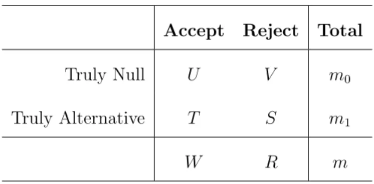
Table 1: Possible outcomes fromm hypothesis tests when the true states of being either null or alternative are fixed and known.

Accept Reject Total

Truly Null U V m0

Truly Alternative T S m1

W R m

for the number of comparisons needed to test all genes. In the multiple testing literature, the outcomes of the m tests are usually delineated as falling into one of four types, as shown in Table 1 (Benjamini and Hochberg 1995).

The random variables U and S represent the two kinds of correct conclusions that are made, while V is the number of false positives (Type I errors) and T is the number of false negatives (Type II errors) that occur. Two parameters that are often used to describe error when conducting multiple tests are the family-wise error rate (FWER) and the false discovery rate (FDR). Different methods have been proposed for either controlling or estimating one of these error rates in analyses containing multiple tests.

The FWER is defined as the probability of having at least one Type I error among the rejected hypotheses, P r(V _≥1). Classically, a Bonferroni correction is employed as a single-stepp-value adjustment, where for the ith test ˜pi = min(m·pi,1). This provides

(20)

Ge et al. (2003). Holm (1979) suggested a similar step-down procedure that applies successively less stringent adjustments to the ordered values, pr1 ≤pr2 ≤. . .≤prm

˜

pri = max

l:1,...,i

min((m₋l+ 1)_·prl,1)

(1.1)

Westfall and Young (1989) proposed a resampling-based procedures for controlling the FWER when correlation exists among the hypothesis tests, that defines the adjusted

p-values as

˜

pri = max

l:1,...,i

P r( min

h:l,...,mPrh ≤prl|m1 = 0)

. (1.2)

Even though this definition conditions on the fact that all genes are truly null (m1 = 0), strong control of the FWER was proved for any realization of null and alternative hy-potheses (Westfall and Young 1993). For each of these controlling procedures, a corre-sponding estimate of the FWER exists for every p-value cut-off to a rejection region.

The FWER error rate is often criticized as being too stringent a criterion when rejecting more than a few hypotheses. For this reason, methods that focus on the FDR have received much attention in the microarray literature where thousands of genes are tested simultaneously. The FDR was originally defined by Benjamini and Hochberg (1995) to be the expected rate of false positives among the rejected hypotheses E[V

R]

where in order to be finite, the ratio V

R is defined to be zero when R =V = 0.

F DR=E

V

R|R >0

P r(R >0) (1.3)

(21)

is small so the difference between these alternative definitions is negligible. Linear step-up procedures to control the FDR were proposed by Benjamini and Hochberg (1995) for independent tests and then by Benjamini and Yekutieli (2001) for correlated tests. To estimate the positive FDR of a given rejection region Storey and Tibshirani (2003) proposed several methods based on the following formulation, and applied the term “q -value” as the following error rate of ap-value and its corresponding estimate

q(p) = inf

{Γ:p∈Γ}pF DR(Γ)

ˆ

q(p) = min

{pΓ≥p}

ˆ

m0 ·pΓ #_{pi ≤pΓ}

where Γ is the rejection region applied marginally to all hypothesis tests. It should be noted that the FDR controlling and estimating procedures can be applied to either parametrically derived p-values or empirical p-values obtained from resampling. Because of correlation in gene expression, the resampling-based procedures for estimating error rates have been shown to be more powerful in example microarray datasets (Ge et al. 2003; Reiner et al. 2003).

1.4 Gene categories

(22)

sequence information along with names, species of origin, and references for every entry. In addition SWISS-PROT provides a set of keywords, based on a taxonomy that includes pathways, diseases and general biological processes. SWISS-PROT also provides cross references to other gene classifications, like that of InterPro and the Protein Families (Pfam) databases. Pfam has used multiple sequence alignment and hidden Markov mod-els to identify 8296 “protein families” that share homology-based domains in their protein amino acid sequence (Sonnhammer et al. 1997). From these sources of information, a functional category can be formed by the set of genes which share a annotation feature, such as a SWISS-PROT keyword or a Pfam domain.

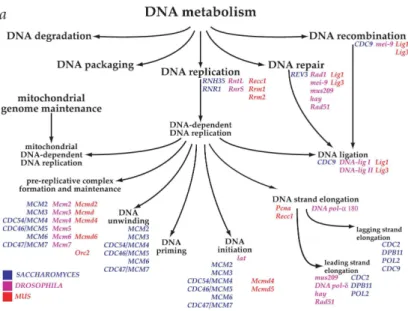
More recently, the Gene Ontology Consortium (GO) has developed a comprehensive vocabulary of gene annotation that is separated into three domains of classification: Biological Process, Cellular Component, and Molecular Function (Ashburner et al. 2000). In each domain, the ontology is structured as a directed acyclic graph (DAG), with a hierarchy of terms that vary from broad levels of classification (e.g. ‘DNA Metabolism’) down to more narrow levels (e.g. ‘leading strand elongation’), as represented in Figure 1. For each GO term, a functional category is generally defined as containing the set of genes annotated directly to the node or to any terms that occupy descendant nodes in the ontology (Ashburner et al. 2000; Zhou et al. 2002). For example, from the subset of the Biological Process ontology shown in Figure 1, the mouse gene Lig1 would be in categories for ‘DNA ligation’, ‘DNA recombination’, ‘DNA repair’, ‘DNA-dependent DNA replication’, ‘DNA replication’ and the parent node ‘DNA metabolism’.

(23)

Figure 1: Example of the structure of Gene Ontology from Ashburner et al. (2000). A subset of the Biological Process DAG is shown with gene members from 3 different species

in (Kanehisa 1997). While a KEGG pathway contains considerably more information than mere membership of the genes, testing procedures are not available for the complex interactions of proteins networks, and as such whole or partial pathways may be reduced to functional categories as a way of examining their general associations to a response of interest in a microarray dataset.

(24)

process at best, and frequently the list of significant genes is too long to develop a parsimonious understanding of the role of biological function.

A number of publications and software packages in the last three years have pro-posed simple hypothesis tests for the differential expression of gene categories, in which a secondary analysis is performed once the list of significant genes has been determined. The most common method looks for over-representation, or “enrichment”, of the category within the gene-list using techniques traditionally employed in the analysis of contingency tables (e.g. Fisher’s Exact Test). Draghici et al. (2003) and Kim and Falkow (2003) were two of the first publications to describe the tests for over and provide tools for conduct-ing tests on lists of genes: Onto-Express and LARK respectively. Subsequently, a series of online tools have also been developed including GOStat from Beißbarth and Speed (2004), FatiGO (Al-Shahrour et al. 2004), EASE (Hosack et al. 2003), and FuncAssoci-ate (Berriz et al. 2003). Several other softwares have been developed that can also display the tests of over-representation across the DAG structure of a GO ontology: MAPPfinder (Doniger et al. 2003), GoMiner (Zeeberg et al. 2003), GoSurfer (Zhong et al. 2004), and GO Tree Machine (Zhang et al. 2004). In all of these software packages, testing for over of a keyword is done by appealing to standard sampling theory. Assume a total of m

genes are on the array, and g of them are annotated to the term of interest. The p -value for having xgenes make a gene-list of length k is derived from the hypergeometric distribution as

P(X_≥x_|m, g, k) =

min_X(g,k)

i=x g i

m−g k−i

m k

(1.4)

(25)

the traditional tests of the difference in proportions, and in some, tests are also conducted by permuting the gene assignments of categories (Berriz et al. 2003; Zhong et al. 2004). In this way, the random sampling of genes assumed in the parametric tests is induced, but the relatedness of overlapping categories is accounted for in the estimated error rates for multiple testing. Other parametric tests have been proposed that use a more continuous measure of gene-specific significance (e.g. Boorsma et al. (2005); Goeman et al. (2004); Kim and Volsky (2005)), and permutation-based tests have been proposed using similar statistics (Mootha et al. 2003; Virtaneva et al. 2001). The gene-list enrichment tests have been criticized for having ill-defined null hypotheses (Allison et al. 2006) and for making assumptions inappropriate for microarray data (Barry et al. 2005), but are increasingly becoming a default tool for testing functional categories in differential expression studies. A full discussion of the various hypothesis testing methodologies and their associated assumptions will be given in the following chapters.

1.5 Resampling-based tests

(26)

2003 | 2004 | 2005 | 2006

Cumulative Number of Publications

All Gene−list Array perm. Gene perm.

0

200

400

600

800

1000

Apr−Jun Oct−Dec Apr−Jun Oct−Dec Apr−Jun Oct−Dec Apr−Jun

Figure 2: The cumulative number of citations of gene category tests plotted quarterly since 2003. Results are shown for ‘gene-list’ methods, resampling based methods that permute either gene- or array-assignments, and the union of the three sets (see Chapter 3 for a full discussion of these methodologies). Citations were obtained from ISI Web of Knowledge on 8/15/06.

(27)

widely implemented in statistical applications.

1.5.1 Permutation testing

Permutation of observed data was originally proposed by R.A Fisher in the 1930s as a theoretical argument for justifying the t-distribution in a two-sample location problem, and has been utilized in deriving the null distribution for many non-parametric statistics (Hollander and Wolfe 1999). Specifically, if a statistic is written as some function of independent units of the observed data, tobs =T(x1, . . . , xn), an empirical p-value can be

simply obtained from the n! reorderings of the data, x∗

1, . . . , x∗n

p= # of permutations where T(x∗1, . . . , x∗n)≥tobs

n! (1.5)

For many experimental designs, like the two-sample comparison, there will be fewer than

n! unique values T∗ _{can take, which leads to a more discrete distribution of empirical}

p-values. Also, for large n it is often times sufficient to approximate p with a smaller number of randomly selected permutations

p=. 1 +

PK

k=1I(t∗k≥tobs)

K + 1 (1.6)

Under this definition, p follows the discrete uniform distribution for the null hypothesis induced via permutation. For many uses of permutation tests, the induced null may not be expressly stated nor confirmed as pertaining to the research question of interest.

(28)

component analysis (Landgrebe et al. 2002), and similarity scores for gene categories (Rahnenf¨uhrer et al. 2004). When applying permutation-based methods to microarray analysis, it is important to recognize what null hypothesis is induced by the randomiza-tion scheme, and whether it is appropriate for the given task (Allison et al. 2006).

1.5.2 Bootstrap testing

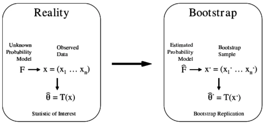
The general bootstrap method was proposed by Efron (1979) and is based on the pre-sumption that the observed data is generated from an unknown probability model, F, as depicted in Figure 3 as adapted from Efron and Tibshirani (1998). If one defines

θ =T(F) as a parameter of interest that is some function of the underlying distribution of the data, the plug-in principle suggests that a simple estimate of θ can be obtained from the empirical distribution function, ˆF, that is a corresponding estimate of F. In order to make inference on θ from ˆθ = T( ˆF), resamples of the data are drawn from ˆF

yielding replicates of the statistic _{θˆ∗_}_.

(29)

Figure 3: Schematic of the bootstrap philosophy recreated from page 87 of Efron and Tibshirani (1998). In order to know the properties of a test statistic when there is an unknown probability model, F, that generates the observed data, x, resamples taken from the empirical distribution of the data gives replicates of the statistic that allow one to approximate its distribution.

biases in the statistic (Efron 1981). Improvements to these basic bootstrap intervals can be made by “double bootstrap methods” where the bias of using resamples of the observed data is measured by resampling a second time from the bootstrap replicates (Beran 1987). For all interval estimates that can be obtained from bootstrap methodologies, there exists a corresponding hypothesis test that looks for the inclusion of null value of the statistic, θ0 = EH0[ˆθ] in the interval. The proper coverage of any of these intervals

may not be precise for smalln because the discreteness of ˆF might prevent it from being a good estimate ofF, and smoothing methods may be employed to improve performance (Polansky and Schucany 1997).

(30)

(31)

2 Testing categories by structured permutation

2.1 Introduction

(32)

category show a consistent but modest association to the response of interest, they may fail to reach the criteria for inclusion in the gene list when issues like multiple testing are accounted for. In this case, the accumulation of effects across a category would go unnoticed when examining only membership in the list. A much bigger concern with gene-list enrichment tests is that do not take into account the possible correlation among genes within and outside a category. For categories with highly correlated genes, the true Type I error will be substantially higher than the reported p-value, resulting in anti-conservative tests. These drawbacks suggest the importance in finding an improved method of testing gene categories. In the following chapter a framework is presented for testing the associations of a functional category of genes in a more valid manner.

2.2 The SAFE framework

(33)

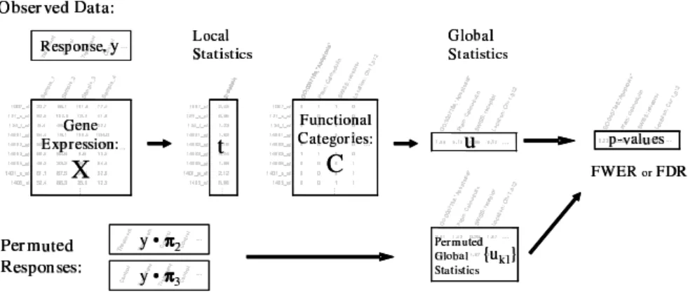
Figure 4: Schematic for the significance analysis of function and expression (SAFE). The observed data consist of a matrix of normalized expression esti-mates,X, a response vector, y, and gene category assignments defineda priori in a matrix C. For the observed and permuted data, gene-specific local statis-tics and category-specific global statisstatis-tics are computed such thatp-values are obtained for each category along with estimated error rates.

other genes. The significance of the global statistics is assessed by repeatedly permuting the array assignments and recomputing local and global statistics. In this manner, the correlation between all genes is maintained by holding the gene expression data constant. Furthermore, the relationships among categories which contain overlapping genes will be preserved, which is important for multiple testing considerations.

(34)

2.2.1 The observed data

The following notation is introduced for describing DNA microarray data and gene cate-gory tests. In the following chapter we will demonstrate how this general form allows the variety gene category tests proposed in the literature to be presented in a unified way. Let the observed expression data for m genes and n samples be given by the matrix x, where the expression of the i-th gene in the j-th sample is xij. For the expression values

of thei-th gene, the row vector that corresponds is given asxi∗, and for the j-th sample,

the column vector is written asx_∗_j. The term “gene” is used to generically identify a row of x but can also correspond to a probe or probeset for a transcript, depending on the array platform and pre-processing steps. Therefore, a single gene might be represented by different transcripts and appear as multiple rows ofx. Extensions of SAFE are proposed in Chapter 4 that would give an appropriate way to account for the multiple represen-tation of a gene on an array. We will generally assume that suitable normalization and other data pre-processing steps as described in Chapter 1 (cf. Dudoit et al. (2002); Li and Wong (2001)) have been performed. The relevant sample information is represented by the response vector y, where each element, yj, can be a group assignment based on

the experimental design or a continuous measure. For some experimental designsyj may

be more than a scalar value, as seen in the survival analysis performed in section 2.3.3. Prior to SAFE analysis, a collection of functional categories of interest must be spec-ified. When a total of Lcategories are under examination, the gene membership can be stored in a m_×L matrix of indicators, where cih= 1 if genei belongs to category hand

(35)

X, y, and C.

2.2.2 Statistics and permutation

Two statistics must be specified in SAFE: The first is based on the experimental design, and termed a “local” statistic t = T(xi∗,y), measuring the association between the

expression profile of geneiand the response vector. In a study whereyj ∈ {0,1}denotes

one of two experimental conditions, one might use either a t-statistic, a non-parametric statistic, or some other measure for comparing _{xij : yj = 0} and {xij : yj = 1} (e.g.

fold-change.) As genes in the same category might exhibit changes in either direction, a two-sided local statistic such as the absolute value of a t-statistic would be the natural choice in a exploratory analysis unless the underlying biological suggests a concerted direction of differential expression in a category of interest.

The global statistic assesses how the distribution of local statistics within a category differs from local statistics outside the category. For a given category, h, the statistic

u=U(t1, . . . , tm; cl) measures some difference between the local statistics of genes within

category, namely _{ti : cih = 1}, and the local statistics of genes in the complement of

the category, namely _{ti :cih = 0}. Typically little is known about the joint density of

the local statistics. For this reason we favor rank-invariant choices for U, such as the Wilcoxon rank sum (Virtaneva et al. 2001) as likely to retain reasonable power under a variety of experimental designs.

(36)

per-mutations in Π reflect the underlying experimental design, including pairing of samples, blocking, or other sampling-based constraints. For many experimental designs, all n! permutations are permissible, although fewer equivalent permutations of the response vector may exist (as in the two-sample problem). For datasets of even modest size, it may not be computationally feasible to use all permutations, and the elements of Π are chosen as a random sample from all permissible permutations. The elements of Π can be represented as permutations of the integers _{1, . . . , n_}, so that Π is stored an n_×K

matrix. We will restrictπ1 to be the identity permutation, corresponding to the observed order of the response vector.

For each gene and each permutation πk ∈ Π, let tik = T(xi∗,y·πk) be the value of

T when the response is permuted according to πk. Here y·π = (yπ(1), . . . , yπ(n)) is a

re-ordering of the components of y according to π. Let u be the K _×L matrix with entries ukh for the h-th functional category under permutation πk. Permutation-based

p-values are computed for each category as ph = K−1PK_k₌₁I{ukh ≥ u1h}, with I{·}

denoting the indicator function. By restricting π1 in this manner, the empirical p-value will appropriately follow a discrete uniform distribution under permutation.

2.2.3 Error rate estimation and plots

(37)

and Tibshirani 2003; Yekutieli and Benjamini 1999) for the set of categories that fall within a given rejection region. First, the matrix of global statistics is converted into a

K_×L matrix of empirical p-values with elements

pkl =

1

K

X

h=1

I_{uhl ≥ukl} (2.1)

In this way, every column, and thus every category, has empirical p-values that range from _K1 to 1. If we define a rejection region by the interval, [0, p], the Westfall-Young estimate of the FWER can be written as

\

F W ERW Y(p) = max l:pl≤p

1 K K X k=1 I min

h:ph≥pl

pkh ≤pl

(2.2)

Thus each p-value that occurs in the rejection region (indexed by l in equation 2.2) is compared to the minimum permuted p-value of all categories less significant. Then, the maximum of these comparisons is taken as the FWER estimate as part of the step-down procedure.

To estimate the FDR through resampling, Yekutieli and Benjamini (1999) proposed the following statistic for a similarly defined rejection region.

\

F DRY B(p) = min l:pl≥p

1

K₋1

K

X

k=2

_ˆ

Vk(pl)

ˆ

Vk(pl) + ˆS(pl)

(2.3)

The functions ˆVk(·) and ˆSk(·) correspond to estimates of the number of true and false

positives as presented in Table 1, and are defined as ˆVk(p) = PlL=1I(pkl ≤ p) and

ˆ

S(p) = ˆV1(p)₋ _K1₋₁PK_k₌₂PL_l₌₁I(pkl ≤p). The minimum is taken among the categories

(38)

Storey and Tibshirani (2003) has also proposed a resampling-based method for esti-mating the FDR. In addition to defining a rejection region, another region is required that is thought to contain almost entirely true null hypotheses, [p0,1].

\

pF DRST(p) = min l:pl≥p

_W₁₍_p₀₎_· 1

K−1

PK

k=2Rk(pl) 1

K−1

PK

k=2Wk(p0)·R1(pl)

(2.4)

where Rk(p) =PLl=1I(pkl≤p) and Wk(p) =PLl=1I(pkl ≥p) also represent estimates of

the corresponding unknown outcomes given in Table 1.

Non-resampling based error estimates, such as the traditional FDR step-up procedure by Benjamini and Hochberg (1995) and the basicq-value estimate (Storey and Tibshirani 2003) can be readily applied to _{ph}. However, these methods may be less appropriate

for the unknown dependence among categories. Permutation enables control of multiple-testing error rates among correlated tests without the need to adopt overly conservative procedures (e.g. Benjamini and Yekutieli (2001)). Permutation-based control of the FWER exploits positive correlation among the global statistics for categories with over-lapping genes, while a Bonferroni threshold in this case will be highly conservative. In our examples using the GO ontologies, the dependence between some categories (nodes) is very strong, as many related categories contain identical or nearly identical sets of genes.

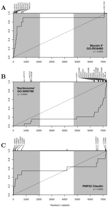
In addition to a p-values and error rate estimates, the significance of each category can be presented in the form of a SAFE-plot. For category h, the SAFE-plot displays the empirical cumulative distribution function (eCDF) of the ranked local statistics _{ti :

cih = 1}. A category that contains many genes that are more differentially expressed

(39)

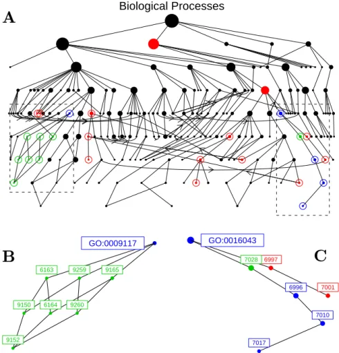
in the eCDF from the diagonal. In cases where an absolute value is taken to create a two-sided local statistic, such as _|t_|in the two-sample comparison, ranking genes by the untransformed statistic will reveal the directions of differential expression for individual genes in the category. Labeled tick marks along the top of the graph allow the investigator to observe the genes most responsible for a categories significance. When gene categories have additional structural relationship such as the hierarchy of GO ontologies, we find it is also useful to display the SAFE significance results within a graphical representation of the structure. For GO, SAFE results can be plotted across the directed acyclic graph to identify the relationships among significant categories.

2.3 Examples from a microarray dataset

To demonstrate the applicability and flexibility of SAFE, gene category analyses were conducted for several responses in a study of human lung carcinomas by Bhattacharjee et al. (2001). A total of 202 lung specimens were assayed with hgu95Av2 oligonucleotide arrays (Affymetrix, Santa Clara, CA). The data consisted of 16 normal tissues and 186 tumors, sub-classified as adenocarcinomas (n = 139), pulmonary carcinoids (n = 20), small-cell lung carcinomas (n = 6), and squamous cell lung carcinoma (n = 21). Addi-tional clinical information, including survival times, were available for 125 of the adeno-carcinomas. Our significance analyses focused on three comparisons: (1) a two-sample comparison of normal versus cancerous samples; (2) an ANOVA model comparing cancer subtypes; and (3) a survival analysis within the adenocarcinoma subgroup.

(40)

expression estimates were obtained from the dChip v1.3 software from Li and Wong (2001). In keeping with the terminology above, each hgu95Av2 probeset is referred to as a “gene” even though in many cases multiple probesets are known to correspond to the same gene. Arrays were normalized by quadratic scaling to an artificial array of median expressions for each gene (Yoon et al. 2002). Genes were filtered out when called absent by the Affymetrix MAS5.0 algorithm in more than half the samples of every tissue type. These preprocessing steps resulting in expression estimates for 202 microarrays and 7299 genes.

Each SAFE analysis involved a common set of functional categories derived from GO and Pfam. Annotations for the hgu95Av2 array are available in the NetAffx (Liu et al. 2003) format from http://www.affymetrix.com. GO gene categories sets were generated from the hierarchical structure of an ontology in the standard manner (Ashburner et al. 2000; Beißbarth and Speed 2004; Zeeberg et al. 2003), using simple algorithms to create the C matrix of indicators required for the SAFE analysis. The 7299 expressed genes had a total of 3860 GO nodes and 1811 Pfam domains linked to them. In order to retain power in this example, only categories of a sufficient size are considered: including 120 cellular component nodes having at least 10 expressed genes, and 207 biological process nodes and 132 molecular function nodes having at least 40 expressed genes. Pfam gene categories were limited to the 176 domains annotated to at least 10 expressed genes.

For each response vector, an appropriate local statistic was chosen, the Wilcoxon rank sum was used as the global statistic,

u=

m

X

i=1

(41)

(42)

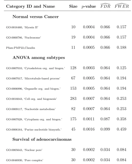
Table 2: Significant GO and Pfam gene categories for the three comparisons in the Bhattacharjee et al. (2001) lung carcinoma study. For each response, the largest subset of all categories with a FDR _≤ 0.1 is reported along with the corresponding FWER estimates.

Category ID and Name Size p-value \F DR F W ER\

Normal versus Cancer

GO:0016460, ‘Myosin II’ 10 0.0004 0.066 0.157 GO:0000786, ‘Nucleosome’ 19 0.0004 0.066 0.157 Pfam:PMP22 Claudin 11 0.0005 0.066 0.188

ANOVA among subtypes

GO:0007010, ‘Cytoskeleton org. and biogen.’ 128 0.0003 0.064 0.125 GO:0007017, ‘Microtubule-based process’ 67 0.0005 0.064 0.194 GO:0006996, ‘Organelle org. and biogen.’ 153 0.0005 0.064 0.194 GO:0016043, ‘Cell org. and biogenesis’ 283 0.0007 0.064 0.253 GO:0009117, ‘Nucleotide metabolism’ 82 0.0007 0.064 0.253 GO:0007028, ‘Cytoplasm org. and biogen.’ 175 0.0011 0.087 0.358 GO:0006164, ‘Purine nucleotide biosynth.’ 45 0.0016 0.099 0.459

Survival of adenocarcinomas

(43)

2.3.1 Two-sample comparison

As a first examination of differential expression, a two-sample comparison was made between normal and tumor samples using the absolute value of the Welch t-statistic as the local statistic. Using the SAFE nomenclature, whereyj = 1 if the array corresponded

to a tumor sample, and yj = 0 if it corresponded to a normal sample, the local statistic

for the i-th gene is written as

ti = |

¯

xi,1−x¯i,0|

q

s2 i,1

n1 +

s2 i,0

n0

(2.6)

wherenc=Pn_j₌₁I(yj =c), x¯i,c = _n1_cPn_j₌₁xij·I(yj =c) , and s2i,c = nc1−1

Pn

j=1(xij− ¯

xi,c)2·I(yj =c) c= 0,1 . Observed values ranged from very close to 0 to 18.4. Under

10,000 permutations of the array assignments, 1235 genes (17% of all tests) achieved a minimum empirical p-value 0.0001. With such dramatic differences between normal and tumor tissue producing a long list of differentially expressed genes, obtaining useful biological conclusions requires a broader perspective.

Among the 635 functional categories we considered in SAFE, three categories had

(44)

under-expressed, (p = 0.0005).

These results demonstrate the various directions of differential expression that can be detected in a two-sample SAFE analysis. Since no overlap in gene membership occurs among the three categories, they can be separate findings. Several of the genes that are present in these categories have been associated with other forms of cancer, however the SAFE results suggest that families related genes may be dis-regulated in cancer.

(45)

MYL9 MYL6 MYH11 MYH11 MRCL3 MYH11 MYH11 MYH9 MRLC2 MLC1SA

0 1000 2000 3000 4000 5000 6000 7000

0.0 0.2 0.4 0.6 0.8 1.0 Ranked t−statistic GO:0016460 p = 0.0004 ‘Myosin II’

MYST3 MYST3 H3F3B H1FX HIST1H2BK H2AFY HIST1H1C H2AFZ H1FX HIST2H2BE H1F0 H1F0 32609_at HIST1H2BM HIST1H2BL H2AFX HIST1H2BD H1F0 286_at

0 1000 2000 3000 4000 5000 6000 7000

0.0 0.2 0.4 0.6 0.8 1.0 Ranked t−statistic GO:0000786

p = 0.0004 ‘Nucleosome’

EMP3 PMP22 EMP2 CLDN18 CLDN5 EMP1 CLDN10 CLDN7 CLDN4 CLDN3

0 1000 2000 3000 4000 5000 6000 7000

0.0 0.2 0.4 0.6 0.8 1.0 Ranked t−statistic PMP22 Claudin p = 0.0005

Figure 5: SAFE-plots for significant categories in normal versus tumor. Welch

(46)

2.3.2 ANOVA

To look for differences in gene expression among the four cancer subtypes, the stan-dard ANOVA F-statistic was used. A scaled F-statistic can be defined in the SAFE nomenclature using yj ∈ {1,2,3,4} for each of the four tumor classifications

ti =

P4

c=1nc(¯xi,c −x¯¯i)2

(Pn_j₌₁(xij−x¯¯i)2−P4_c₌₁nc(¯xi,c−x¯¯i)2)

(2.7)

where nc = Pnj=1I(yj = c), x¯i,c = _n1_cPnj=1xij ·I(yj = c) c = 1,2,3,and 4 , and

¯¯

xi = 1_nPn_j₌₁xij . For a total of 2689 genes (37% of all tests) the observed local statistic

achieved the minimum empiricalp-value (p= 0.0001). The substantial differences in ex-pression profiles between cancer subtypes provided the basis for successful discrimination in the original report (Bhattacharjee et al. 2001). Here we employ SAFE to establish which functional categories consistently differ in expression across cancer subtypes.

Eight biological process nodes (havingp-values_≤0.0019) met the criterion of\F DR_≤

(47)

Biological Processes

9165 9259 6163

9150 6164 9260

9152

GO:0009117

6997 7028

7001

6996

7010

7017

GO:0016043

(48)

2.3.3 Survival analysis

Censored survival data were available for 125 subjects with adenocarcinomas, with 71 observed deaths and 54 censored observations. The association between a gene’s expres-sion and survival was assessed with a univariate Cox proportional hazard model (Cox 1972). Let yj represent the censored failure time for the j-th array, using the pair of

values yj = {tj, dj} with tj measuring the time to event and letting dj = 1 if a death

occurred, and dj = 0 if the corresponding subject was censored. In the Cox model,

regression coefficients are estimated by the maximum of the partial likelihood

ˆ

βi = sup βi

L(βi) = sup βi

n

Y

j=1

dj ·exp(xij·βi)

P

r∈Risk(tj)exp(xir·βi)

(2.8)

where Risk(tj) refers to the riskset for that time consisting of all subjects for whom a

death or censored outcome had not yet been observed. Although ˆβi does not have a

closed form, the log likelihood is strictly concave, and can thus be solved quickly for all genes using Newton-Raphson iteration or a bisection algorithms.

The local statistic is the Wald-type statistic

ti = |

ˆ

βi|

b

se( ˆβi)

(2.9)

where the standard error of the regression estimate is approximated by the observed information of the partial likelihood

b

se( ˆβi) =

−∂2

∂β2

i

logL(βi)_|βi= ˆβi

−1 2

(2.10)

(49)

correction (all the common FDR and FWER estimates presented in this proposal were greater than 0.2). The data provide an example where standard gene-specific approaches fail to provide useful conclusions because no effects are strong enough to pass the multiple-testing criterion. We then applied the SAFE approach, which is sensitive to the aggregate effect of genes with related biological functions.

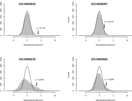
After accounting for multiple testing, two related GO cellular component nodes were significant (Table 2): GO:0005643 ‘Nuclear pore,’ and GO:0046930 ‘Pore complex.’ How-ever, the nodes for ‘Nuclear pore’ and ‘Pore complex’ contain an identical set of 30 genes and should be considered a single finding (p= 0.0002). Likewise, the parental node, ‘Nu-clear membrane,’ was marginally significant (p= 0.0012,\F DR= 0.106) but shared 30 of 51 genes with the other nodes. An additional SAFE-plot for the genes unique to ‘Nuclear membrane’ (not shown) indicates that only the nuclear pore genes are associated with survival.

(50)

2.4 Discussion

These examples demonstrate the applicability of SAFE to a variety of experimental de-signs and measures of gene-specific differential expression. It is further observed that significant categories can be found both when many gene-specific associations are ob-served across the array or with few significant genes.

Although both SAFE and the gene-set enrichment analysis (GSEA) proposed by Mootha et al. (2003) are two-stage procedures that employ array permutation, there are two distinctions to be made. First, GSEA uses a Kolmogorov-Smirnov type global statistic that looks for any general difference between the empirical CDFs of category and complement local statistics. In doing so, this method has been criticized for being sensitive to departures from the null that do not necessarily reflect increased associa-tion of expression and response values in the category (Damian and Gorfine 2004). For instance, a category containing local statistics that are very non-significant but similar in magnitude (e.g., t-statistics all close to 0 in a two-sample experiment) will also be rejected by GSEA.

(51)

(52)

Standardized Wilcoxon

Counts

−5 0 5 10

0 200 400 600 800 1000

p = 2e−04 GO:0005643

Counts

−5 0 5 10

0 200 400 600 800 1000

p = 0.0479 GO:0008287

Counts

−5 0 5 10

0 200 400 600 800 1000

p = 0.0937 GO:0005578

Counts

−5 0 5 10

0 200 400 600 800 1000

p = 0.0589 GO:0000502

(53)

3 A comparison of gene category tests

3.1 Introduction

Beginning with Virtaneva et al. (2001), a number of publications have proposed tests for assessing the association between response and gene categories. The most commonly employed tests are designed to begin with a list of significant genes. A secondary analysis then looks for over-representation, or enrichment, of genes within the category on the gene-list, using Fisher’s Exact Test or other tests of 2 x 2 contingency tables (see Section 1.4 for a list of methods and softwares). Other approaches examine the significance of genes using more direct comparisons of the gene-specific measures of DE, thereby avoiding any need for intervening gene lists. In these methods, tests are constructed either for an average difference of gene-specific statistics (Boorsma et al. 2005; Kim and Volsky 2005), or using classical rank-based procedures for two-sample comparisons (Barry et al. 2005; Ben-shaul et al. 2005; Mootha et al. 2003). Herein we describe how the existing gene category methods can also be broadly sorted according to the null hypotheses they test against.

(54)

formal definition of the underlying null hypothesis and a proper demonstration of Type I error have not been provided for many of the various methods in the literature.

3.1.1 Contributions

In this chapter we provide a careful and rigorous analysis of gene category testing by first defining a general framework. Presenting and contrasting existing methods in this manner allows us to identify two distinct classes that are defined by the null hypothe-ses they assume or induce. Several shortcomings of these methods are revealed through derivation and through simulations from an example dataset. We then propose an al-ternative approach to hypothesis testing that can overcome these shortcomings so that it provides more power while demonstrating proper coverage under the null hypothesis. This approach can also be applied to a wider set of experimental designs.

(55)

gene-specific statistics. Conversely, array permutation methods constitute a second class of gene category tests, having been proposed with the stated intention of preserving the correlation in expression observed among genes (Barry et al. 2005; Mootha et al. 2003). We next define an important property of gene-specific statistics that is necessary for proper coverage under array permutation. When this property is met, the induced null hypothesis is that gene-specific test statistics are dependent, yet approximately identically distributed according to no association with the response. Gene category methods that rely on this null are shown to provide better coverage in simulated data.

(56)

3.2 A general framework for gene category tests

3.2.1 Notation and framework

To describe the variety of gene category tests in a unified way, we will continue to refer to the observed expression data as x, and the response as y as in Section 2.2.1. When we regard an unrealized expression matrix as a collection of random variables, we will use uppercase versions of the standard notation, i.e., X, Xij, Xi∗ and X∗j.

To more easily derive the properties of tests, a single gene category will be represented by a subset C _{⊆ {}1, . . . , m_} such that i _∈ C if and only if gene i is a member of the category. The size of a category C will be denoted by mC = Pm_i₌₁I(i ∈ C). For

any category C, the complementary set of genes will be denoted by ¯C and be of size

m_C¯ =m−mC.

We also adopt the terminology in the previous chapter, where hypothesis tests of gene categories can be viewed as a two-stage procedure (see Box 1). In the first stage, a local statistic measures the association between the expression profile of each gene and the response. We denote the local statistic of gene i by Ti = T(Xi∗,y) and let ti

(57)

response and expression. In the example local statistics for a two-condition experiment that are given above, the related parameters would be a scaled difference and a ratio of population means, respectively. Properties of local statistics are examined more fully in Section 3.5.3.

In the second stage of a gene category test, a global statistic is used to compare the local statistics of genes within a category C to those in the complement. We denote the global statistic for category C by U = U(T1, . . . , Tm : C), and in the following sections

(58)

Box 1: Common elements of gene category tests

Gene category tests are typically two-stage procedures requiring the

follow-ing statistics:

• A local statistic that measures the association between response (e.g.

experimental condition) and expression of each gene.

• A global statisticthat compares the local statistics within a category

to those of its complement.

Two classes of hypothesis tests are typically designed for each global statistic:

1. Parametric or rank-based procedures that assume independent and

identically distributed local statistics, or gene permutation methods

that induce the same null.

2. Array permutation methods which induce a null that maintains the

correlation structure among genes while removing all associations to

the response.

Error rate controlling or estimating procedures address the multiple

(59)

3.3 A Survey of gene category test statistics

Gene category test statistics can be generally be represented as looking for a change in the DE of genes within a category relative to the genes in its complement. In a number of the gene category publications, hypothesis tests are designed from traditional methods for comparing two random samples of data. In these proposals, though, we note that the null hypothesis has not be explicitly defined, and it is rarely discussed whether the necessary assumptions are met in gene expression data. In the following section, we will demonstrate that a particular null hypothesis is assumed by a variety of gene category tests. The tests that fall into this class vary in terms of the global statistics that are chosen, and whether exact or approximate distributions are used to determine p-values, but can be collectively stated as follows.

Definition 1. Class 1 gene category tests are defined by the assumed or induced null

hypothesis. For local statistics T1, . . . , Tm, the null can be stated as

H0 : T1, T2, . . . , Tm are i.i.dwith Ti ∼F (3.1)

where F can take any general form, but is typically thought to correspond to there being

no association between expression and the response of interest.

(60)

statistics are presented below for each case, and a brief description is given of the cor-responding non-resampling based Class 1 tests. We will focus on one-sided forms of the tests because in most applications one is only interested in categories showing increased association with the response relative to what is seen across the array.

3.3.1 A survey of the global test statistics

Categorical Test Statistics

Gene-list enrichment methods have developed as a post hoc means of testing a category once genes with significant amounts of DE have been identified. Let R denote the re-jection region for the local statistics that produces the significant gene list. R might be determined independently from the data, (e.g.,from quantiles of a centralt-distribution), or in a data-dependent manner (e.g., from methods to control the FWER or FDR for the multiple comparison of m genes).

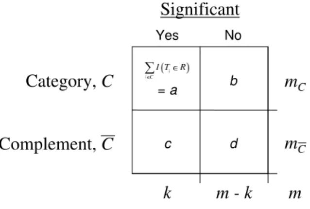
Gene-list enrichment tests only consider the dichotomous outcomes of the m gene-specific hypothesis tests, I_{Ti ∈ R} . The differential expression within C and ¯C is

therefore summarized by a 2_×2 contingency table (Figure 8).

The traditional contingency table tests that have been proposed for gene category analysis include the χ2 _{test of homogeneity, Fisher’s Exact test, and minor variants} of these. In the classical derivation of these tests, the Bernoulli variables I_{T1 ∈

R_}, . . . , I_{Tm ∈ R} are assumed to be independent with the probabilities of rejection

(61)

Figure 8: The results from a gene-specific analysis as given in a 2_×2 table for a category versus its complement. The size of the two gene sets, given by mC

and m_C¯ respectively, are assumed to be fixed quantities. The complete table can then be determined by knowing the number of rejections in the category and either the total number of rejections, k, or the number of rejections in the complement.

look for departures from π_C¯ = πC, where all indicators would be i.i.d. It is worthwhile

to note that the Class 1 null (3.1) is sufficient but not necessary for the dichotomous outcomes to be i.i.d. under a given R. However, (3.1) guarantees the categorical null holds for any possible choice of rejection region.

In several of the gene-list enrichment software packages the χ2 _{test of homogeneity is} proposed as an approximate test for large categories (Beißbarth and Speed 2004; Draghici et al. 2003). The one-sided version of this test is equivalent to the difference in proportions test proposed originally by Pearson (1911), where the global statistic can be written as

UP = ˆπC −πˆ_C¯ = 1

mC

X

i∈C

I_{Ti ∈R} −

1

m_C¯

X

i0_∈_C¯

I_{Ti0 ∈R}. (3.2)

(62)

mC and m_C¯, and a Z-test is performed on a standardized form ofUP.

Fisher’s Exact Test is more commonly applied in gene-list methods, and is noted to be a conditional test based on the total number of rejected hypotheses,K =Pm_i₌₁I_{Ti ∈R}.

Once K is established, the global statistic can be represented as the number of genes in the category that are rejected,

UF =P_i_∈_CI{Ti ∈R} (3.3)

and an exact one-sided p-value is obtained from the hypergeometric distribution. This

p-value is conditional on K, and using it in an unconditional hypothesis test will lead to slightly conservative results, particularly when the category is small (Yates 1984). De-pending on how the gene-list is determined, it is not always clear whether it is appropriate to condition on K, but exact tests are often favored in order to handle small categories. For moderately sized categories, we note there will be little difference between the exact conditional and approximate unconditional tests.

Continuous Test Statistics

(63)

between the two sets.

UD =

1

mC

X

i∈C

Ti−

1

m_C¯

X

i0_∈_C¯

Ti0. (3.4)

Hypothesis tests of UD have been proposed by two similar methods. In one, a t-test is

performed after standardizing by the pooled sample variance of local statistics (Boorsma et al. 2005), while in the second method aZ-test is done afterUD is scaled by the overall

standard deviation in local statistics (Kim and Volsky 2005). For a typical category where mC m, the variance estimates in both methods will be reasonable close, and

similar results will be obtained because of the large number of degrees of freedom of the

t-distribution (df =m₋2).

When using the global statistic in (3.4), the results will be sensitive to the chosen form of the local statistics (e.g., deciding between a t-statistic or its corresponding p-value), and may not be robust to skew or outlying observations. Rank-based global statistics avoid both of these shortcomings, as they are invariant to monotone transformations of the local statistics. The Wilcoxon rank sum test has been implemented in its classical form in the software GOStat (Beißbarth and Speed 2004). In the absence of ties the global statistic is written as

UW =

X

i∈C

Rank(Ti) (3.5)

Under the Class 1 null hypothesis, the discrete CDF of UW is known once mC and m_C¯ are specified. In this case a hypothesis test can be implemented using tables of exact

p-values, or through a Z-test based on a standardized formUW that under independence

will be asymptotically correct for large categories.

(64)

cat-egory test which can also be characterized as testing against the class 1 null (Ben-shaul et al. 2005). However, the Kolmogorov-Smirnov type statistic has been criticized in gene category testing for being sensitive to departures that do not necessarily reflect increased amount of DE in the category (Damian and Gorfine 2004); for example, a category with no DE but with local statistics that all happen to be very close to one another would be identified as significant by these tests. For this reason, we will restrict our focus to the tests of average differences when considering continuous global statistics.

3.4 The effect of correlation on Class 1 tests

In this section we more closely examine the assumption of independent local statistics, and its failure to hold in gene expression data. First, correlation in expression is defined and related to correlation in local statistics. Decompositions of the variances of global statistics demonstrate the effect this dependency has on Class 1 hypothesis tests. A simulation study based on real microarray data exhibits the extreme anti-conservative behavior of these tests in the presence of realistic levels of correlation in expression.

3.4.1 Correlations in expression and local statistics

Let ρX

i,i0 = Corr(X_ij, X_i0_j) be the population correlation between genes i and i0. For

experimental designs with independent arrays, a natural estimate ofρX_i,i0 is the observed

Pearson sample correlation coefficient

ri,i0 =

Pn

j=1(xij−x¯i)(xi0j−x¯i0)

qPn

j=1(xij−x¯i)2·

Pn

j=1(xi0j −x¯i0)2

(65)

where ¯xi =n−1Pnj=1xij.

The distributions of global statistics under the Class 1 null hypothesis are noted to be more directly effected by the correlation between local statistics, namely ρT

i,i0 =

Corr(Ti, Ti0). In the special case thatT takes a linear form T(X_i_∗,y) =Pn

j=1a(yj)·Xij

for some function a(_·), a simple calculation shows that ρT

i,i0 = ρX_i,i0. An example of a

linear local statistic would be an unscaled difference in sample means, e.g., fold change on the log-scale; this choice of local statistic is appropriate if the logarithm is a variance-stabilizing transformation of expression data.

In general, the relationship between the correlations ρX

i,i0 and ρT_i,i0 does not have a

closed analytic form, although it can often be shown numerically to be monotone and quite linear. Monte Carlo simulations of gene expression data demonstrate this linear relationship holds in several standard experimental designs and corresponding measures of DE including t-statistics for two-condition studies and for simple linear regressions (Figure 9). When linearity holds, (3.6) is also a good estimate of ρT

i,i0.

3.4.2 Correlation and Variance Inflation

The effect that the m·(m₂−1) pairwise correlations will have on some of the Class 1 gene category tests can be seen by expanding the variances of particular global statistics. Here, we derive the true variances of the continuous global statistics, UD and UW, and show

how they are greater than what occurs under the i.i.d. assumption when categories have positively correlated gene members. For the categorical global statistics, UF and UP, the

(66)

−1.0 −0.5 0.0 0.5 1.0 −1.0 −0.5 0.0 0.5 1.0 Student’s t−statistic

Local Stat Sample Correlation

−1.0 −0.5 0.0 0.5 1.0

0.0

0.2

0.4

0.6

0.8

Correlation of F’s

Gene Population Correlation

−1.0 −0.5 0.0 0.5 1.0

−1.0

−0.5

0.0

0.5

1.0

CoxPH Wald−type statistic

A B C

Figure 9: Correlations in expression and local statistic were generated by Monte Carlo simulation of Gaussian expression for two genes in several exper-imental designs: (A) Student’s t for a two-sample comparison; (B)F statistic for an ANOVA with 4 groups; (C) Cox-proportional hazard model for relating expression to exponentially distributed survival and censoring times. In each design, the variance of expression in the second gene ranged from 1 to 10 times greater, and data was simulated for n= 40 arrays.

easily presented because of its dependency on both the underlying distribution of local statistics T and also the rejection region R.

For the average difference global statistic, UD, the true variance will differ from that

under the i.i.d. null in class 1 tests by three additive terms

Var[UD] = Vari.i.d.[UD] +

mC −1

mC

ρC +

m_C¯−1

m_C¯ ρC¯−ρC,C¯ (3.7)

where ρC =

1

mC ·(mC −1)

X

i∈C

X

i0∈C i06=i

ρT_i,i0 (3.8)

ρ_C¯ = 1

m_C¯ ·(m_C¯ −1)

X

i∈C¯

X

i0∈C¯ i06=i

ρT

i,i0 (3.9)

ρC,C¯ =

1

mC ·m_C¯

X

i∈C

X

i0_∈_C¯

(67)

The additional terms in the variance are the average pairwise correlation within the cat-egory (3.8), within the complement (3.9), and across the two gene sets (3.10). Moreover, the variance implied by (3.1) (given by Vari.i.d.[UD] in the above equation) is inversely

proportional to mC. Thus, for fixed values of the average correlations, the proportional

variance inflation Var[UD]

Vari.i.d.[UD] will become more pronounced in larger categories. We note

that ρC can vary greatly across categories while ρ_C¯ and ρ_C,_C¯ will close to the average correlation across the array, which is nearer to zero in most datasets. Because of this, cat-egories exhibiting positive correlation will have aUD global statistic with greater variance

than what is assumed under (3.1) leading to an anti-conservative Class 1 test.

For the Wilcoxon rank sum global statistic, it is difficult to relate the effect correlation in expression will have on the exact test ofUW which is based on the discrete distribution

of the ranked sum. Nonetheless, solving for the variance of the statistic provides indirect evidence that the distribution will be misspecified when independence is violated, and also relates to the improper standardization ofUW that occurs in the class 1 approximate

Z-test. In the following theorem, Var[UW] is derived in the special case of jointly Gaussian

local statistics with any correlations_{ρT_}_{. The pdf and cdf of a univariate and bivariate}

Gaussian distribution are denoted by φ, Φ and φ2, Φ2 respectively.

Theorem 1. Let T1, . . . , Tm be identically distributed random variables that follow a

multivariate Gaussian distribution with unit variances and pairwise correlations _{ρT ij}.

Then for some category, C _{⊂ {}1, . . . , m_}, the variance of UW =P_i_∈_CRank(Ti) is given