A novel algorithm for the modelling of complex processes

A novel algorithm for the modeling of complex

processes

José de Jesús Rubio

, Edwin Lughofer

, Angelov Plamen

Juan Francisco Novoa

, Jesus A. Meda Campaña

1 Sección de Estudios de Posgrado e Investigación, ESIME Azcapotzalco,

Instituto Politécnico Nacional

Av. de las Granjas no.682, Col. Santa Catarina, México D.F., 02250, México

(phone:(+52)55-57296000-64497)

(email: [email protected]; [email protected])

2 Department of Knowledge-Based Mathematical Systems,

Johannes Kepler University Linz, Austria,

(email: [email protected])

3 School of Computing and Comunications

Lancaster University

Lancaster LA1 4WA, U.K.

(email: [email protected])

4 Laboratorio de Vibraciones y Rotodinámica, ESIME Zacatenco

Instituto Politécnico Nacional,

(email: [email protected])

Abstract

excessive increasing or decreasing of its gain. The gain of the proposed algorithm is uniformly stable and its convergence is found. The introduced algorithm is utilized for the modeling of two synthetic examples.

Keywords: Recursive least square, Kalman …lter, modeling, complex processes.

1

Introduction

In recent years, the recursive least square and extended Kalman …lter algorithms have been highly utilized in the modeling issue. The recursive least square technique is an adaptive …lter which recursively …nds coe¢ cients that minimize a weighted cost function relating to input signals, and it shows extremely fast convergence [4], [17]. The Kalman …lter strategy is an algorithm that uses a series of measurements observed over time, containing statistical noise and other inaccuracies, and it estimates unknown variables. In the estimation theory, the extended Kalman …lter is the nonlinear version of the Kalman …lter which is the linearization about an estimate of the current mean and covariance [5], [15].

There is some research about recursive least square algorithms. In [21], the least square and backpropagation are combined. The least square method is addressed in [8]. In [16], fuzzy least squares are suggested. The recursive fuzzily weighted least square is used for updating consequent parameters in evolving fuzzy systems [18] and [27], which is extended to a generalized form in [23]. The characteristic of this algorithm is that its gain could converge through the time to a small value. The problem is that the gain could be too small; therefore, the quality of the modeling could become low.

There is some research about extended Kalman …lter algorithms. In [1], [2], [3], and [28], several Kalman …lter algorithms of neural networks are designed. An extended Kalman …lter of a wavelet neural network is utilized in [12]. In [7] and [30], the programming with Kalman …lters is described. An observer-type of Kalman …ltering algorithm is discussed in [11]. In [10], the Kalman …lter of nonlinear processes is designed. Single-pass active modeling …lters are employed in [19], which is used in [20] for the purpose of semi-supervised drift detection. The characteristic of this algorithm is that its gain could grow through the time to a big value. The problem is that the gain could be too big; therefore, the quality of the modeling could become low.

satisfactory modeling.

Furthermore, the Lyapunov technique is employed to guarantee the uniform stability and convergence of the gain in the proposed algorithm. Stability is a method to analyze whether the inputs, outputs, and parameters remain bounded through the time [6], [9], [24], [29], [31]. The uniform stability is stronger than the common stability because the …rst is satis…ed for any initial time, while the second is satis…ed only for a zero initial time.

Finally, the proposed algorithm is compared with the recursive least square and extended Kalman …lter for the modeling of two complex processes. The complex adaptive processes issue has been considered as a well established research area [13], [14], [22].

The paper is organized as follows. The neural network, recursive least square, extended Kalman …lter, and proposed algorithms are detailed in Section 2. The proposed technique is summarized in Section 3. The suggested method is applied for the modeling of two synthetic examples in Section 4. Conclusions and future research are detailed in Section 5.

2

Updating algorithms of a neural network

In this part of the article: 1) the neural network will be explained, 2) the recursive least square, extended Kalman …lter, and proposed algorithms will be detailed for the updating of a neural network, and 3) the stability and convergence of the gain in the proposed algorithm will be analyzed.

2.1

The neural network

Take in account the following unknown complex process:

y(k) = f[x(k)] (1)

with

x(k) = [x1(k); : : : ; xi(k); : : : ; xN(k)]T

= [y(k 1); : : : ; y(k n); u(k); : : : ; u(k m)]T

2 <N 1

N =n+m is the process input, y(k) = _{2 <}is the process output, and f is the unknown behavior of the complex process, f ₂C1.

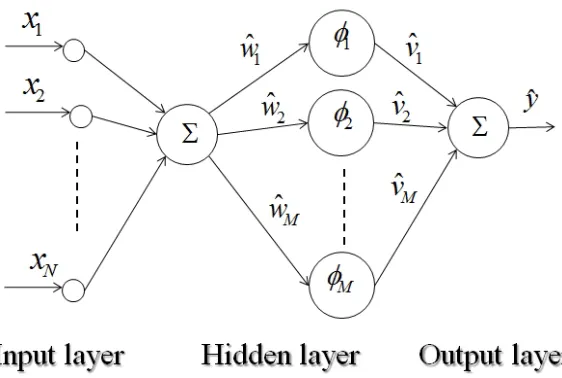
Figure 1: The neural network structure

The structure of the neural network with one hidden layer of this study is shown in Figure 1.

The neural network with the input, hidden, and output layers is written as follows:

b

y(k) = _bv(k) (k) =

M

X

j=1

b

vj(k) j(k)

(k) = [ 1(k); : : : ; j(k); : : : ; M(k)] T

j(k) = tanh(wbj(k) N

X

i=1

xi(k))

j(k) =bvj(k)sech2(wbj(k) N

X

i=1

xi(k)) N

X

i=1

xi(k)

(2)

with i = 1; : : : ; N, j = 1; : : : ; M, x(k)_{2 <}N 1 is the neural network input described in (1), xi(k)2 <, by(k) 2 < is the neural network output, w(k)b 2 <1 M and bv(k) 2 <1 M are the

hidden layer and output weights, wbj(k)2 <, bvj(k)2 <, j(k)2 <, (k)2 <M 1.

The modeling error e(k)_{2 <} is described as follows:

e(k) = _by(k) y(k) (3)

with y(k)and by(k) being described in (1) and (2).

2.2

The recursive least square algorithm

The recursive least square algorithm is described in this subsection for the updating of a neural network. The characteristic of this algorithm is that its gain Gk could converge

through the time to a small value. The problem is that the gain could be too small; conse-quently, the quality of the modeling could become low.

The recursive least square algorithm utilized as the adapting law of the neural network (2) for the modeling of the complex process (1) is represented as follows [25]:

b

(k+ 1) = (k)b _q(1_k)Gk+1a(k)e(k)

Gk+1 =Gk _r(1_k)Gka(k)aT(k)Gk

(4)

with

aT_{(k) = [}

1(k); : : : ; M(k); 1(k); : : : ; M(k)]2 <1 2M

b

(k) = [w_b1(k); : : : ;wbM(k);bv1(k); : : : ;bvM(k)]T 2 <2M 1

r(k) =q(k) +aT_(k)G ka(k)

q(k) =r2+aT(k)Gka(k)2 <

0 < r2 2 < is a forgetting factor, e(k) is the modeling error of (3), j(k) and j(k) are

described in (2).Gk+1 2 <2M 2M is the algorithm gain which is a positive de…nite covariance

matrix, G1 = g1I is the initial algorithm gain, and g1 > 0 is a scalar constant usually big

enough to assure an acceptable convergence, and I _{2 <}2M 2M is the identity matrix.

2.3

The extended Kalman …lter algorithm

The extended Kalman …lter algorithm is described in this subsection for the updating of a neural network. The characteristic of this algorithm is that its gainGk could grow through

the time to a big value. The problem is that the gain could be too big; consequently, the quality of the modeling could become low.

The extended Kalman …lter algorithm utilized as the adapting law of the neural network (2) for the modeling of the complex process (1) is represented as follows [26]:

b

(k+ 1) = b(k) _q(1_k)Gk+1a(k)e(k)

Gk+1 =Gk _r(1_k)Gka(k)aT(k)Gk+R1

(5)

with

aT_{(k) = [}

1(k); : : : ; M(k); 1(k); : : : ; M(k)]2 <1 2M

b

r(k) =q(k) +aT(k)Gka(k)

q(k) =r2+aT(k)Gka(k)2 <

0 < r2 2 < is a forgetting factor, e(k) is the modeling error of (3), j(k) and j(k) are

described in (2).Gk+1 2 <2M 2M is the algorithm gain which is a positive de…nite covariance

matrix, G1 = g1I is the initial algorithm gain, and g1 > 0 is a scalar constant usually

big enough to assure an acceptable convergence, and I _{2 <}2M 2M _{is the identity matrix.}

R1 =r1I, 0< r1 2 <.

2.4

The proposed algorithm

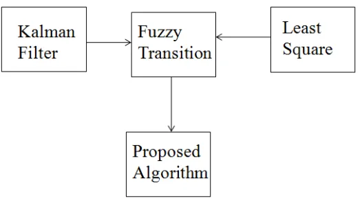
The proposed algorithm is described in this subsection for the updating of a neural network. It presents a fuzzy transition between the recursive least square and extended Kalman …l-ter algorithms with the objective to obtain a bounded gain Gk, maintaining a satisfactory

modeling. Figure 2 shows the proposed algorithm.

Figure 2: The proposed algorithm

The proposed algorithm utilized as the adapting law of the neural network (2) for the modeling of the complex process (1) is represented as follows:

b

(k+ 1) = b(k) _q(1_k)Gk+1a(k)e(k)

Gk+1 =Gk _r(1_k)Gka(k)aT(k)Gk+R1

(6)

with

aT_{(k) = [}

1(k); : : : ; M(k); 1(k); : : : ; M(k)]2 <1 2M

b

r(k) =q(k) +aT(k)Gka(k)

q(k) =r2+aT(k)Gka(k)2 <

0 < r2 2 < is a forgetting factor, e(k) is the modeling error of (3), j(k) and j(k) are

described in (2).Gk+1 2 <2M 2M is the algorithm gain which is a positive de…nite covariance

matrix, G1 = g1I is the initial algorithm gain, and g1 > 0 is a scalar constant usually big

enough to assure an acceptable convergence, andI _{2 <}2M 2M is the identity matrix. 5 rules are used to obtain R1 as a fuzzy transition between the recursive least squareR1 = 0I and

the extended Kalman …lter R1 =r1I as follows:

If0 _kGkk 1₄g1, then R1 =r1I

If 1₄g1 <kGkk ₂1g1, then R1 = 3₄r1I

If 1₂g1 <kGkk ₄3g1, then R1 = 1₂r1I

If 3₄g1 <kGkk g1, then R1 = 1₄r1I

Ifg1 <kGkk, then R1 = 0I

(7)

with 0< r1 2 <.

The stability and convergence of the gain in the introduced algorithm are analyzed by the following Theorem.

Theorem 1 The gain of the proposed algorithm (6) (7) for the updating of the neural net-work (2) (3) is uniformly stable and the following convergence is satis…ed:

lim sup

T!1

1 T

T

X

k=1

bT 1

r(k)Gka(k)a

T_(k)G

kb =r1 (8)

with b = [1;1: : : ;1]T, Gk is the gain of the proposed algorithm described in (6), a(k) and

r(k) are described in (6), and r1 is described in (7).

Proof. Select the following Lyapunov function:

Lk =bTGkb (9)

obtaining Lk as follows:

Lk =Lk+1 Lk =bTGk+1b bTGkb (10)

…ve cases are presented. a) when0 _kGkk 1₄g1, considering (6) and that bTb = 1 gives:

Lk =bTGk+1b bTGkb

=bT h_G

k _r(1_k)Gka(k)aT(k)Gk+r1

i

b bT_G kb

=bT_G

kb bT_r(1_k)Gka(k)aT(k)Gkb+bTr1b bTGkb

Lk = bT_r(1_k)Gka(k)aT(k)Gkb+r1

The following result is obtained:

Lk = bT

1

r(k)Gka(k)a

T_(k)G

kb+r1 (12)

since bT 1

r(k)Gka(k)a

T_(k)G

kb 0 and r1 is small and positive, the gain of the proposed

algorithm is uniformly stable. b) when 1₄g1 <kGkk 1₂g1, considering (6) and thatbTb = 1

gives:

Lk =bTGk+1b bTGkb

=bT h_G

k _r(1_k)Gka(k)aT(k)Gk+3₄r1

i

b bT_G kb

=bTGkb bT_r(1_k)Gka(k)aT(k)Gkb bTGkb+ 3₄r1bTb

= bT 1

r(k)Gka(k)a

T_(k)G

kb+3₄r1

(13)

The following result is obtained:

Lk= bT

1

r(k)Gka(k)a

T_(k)G kb+

3

4r1 (14)

since bT 1

r(k)Gka(k)a

T_(k)G

kb 0 and 3₄r1 is small and positive, the gain of the proposed

algorithm is uniformly stable. c) when 1₂g1 <kGkk 3₄g1, considering (6) and that bTb = 1

gives:

Lk =bTGk+1b bTGkb

=bT hGk _r(1_k)Gka(k)aT(k)Gk+1₂r1

i

b bTGkb

=bTGkb bT_r(1_k)Gka(k)aT(k)Gkb bTGkb+ 1₂r1bTb

= bT 1

r(k)Gka(k)a

T_(k)G

kb+1₂r1

(15)

The following result is obtained:

Lk= bT

1

r(k)Gka(k)a

T_(k)G kb+

1

2r1 (16)

since bT 1

r(k)Gka(k)a

T_(k)G

kb 0 and 1₂r1 is small and positive, the gain of the proposed

algorithm is uniformly stable. d) when 3₄g1 < kGkk g1, considering (6) and thatbTb = 1

gives:

Lk =bTGk+1b bTGkb

=bT hGk _r(1_k)Gka(k)aT(k)Gk+1₄r1

i

b bTGkb

=bT_G

kb bT_r(1_k)Gka(k)aT(k)Gkb bTGkb+ 1₄r1bTb

= bT 1

r(k)Gka(k)a

T_(k)G

kb+1₄r1

(17)

The following result is obtained:

Lk= bT

1

r(k)Gka(k)a

T_(k)G kb+

1

since bT 1

r(k)Gka(k)a

T_(k)G

kb 0 and 1₄r1 is small and positive, the gain of the proposed

algorithm is uniformly stable. e) when g1 <kGkk, considering (6) and that bTb= 1 gives:

Lk =bTGk+1b bTGkb

=bT h_G

k _r(1_k)Gka(k)aT(k)Gk

i

b bT_G kb

=bT_G

kb bT_r(1_k)Gka(k)aT(k)Gkb bTGkb

= bT_r(1_k)Gka(k)aT(k)Gkb

(19)

The following result is obtained:

Lk = bT

1

r(k)Gka(k)a

T_(k)G

kb (20)

sincebT_r(1_k)Gka(k)aT(k)Gkb 0, the gain of the proposed algorithm is asymptotically stable.

Since the uniform stability is weaker than the asymptotic stability [6], [9], [24], [29], [31], considering all cases, the gain of the proposed algorithm is uniformly stable. Now considering all cases. a) when 0 _kGkk 1₄g1, summarize (12) from1 toT:

T

X

k=1

bT 1

r(k)Gka(k)a

T_(k)G

kb=L1 LT +T r1 (21)

multiplying by _T1 and obtaining the limit gives:

lim sup T!1 1 T T X k=1

bT 1

r(k)Gka(k)a

T_(k)G

kb =r1 (22)

b) when 1₄g1 <kGkk 1₂g1, summarize (14) from1 toT:

T

X

k=1

bT 1

r(k)Gka(k)a

T_(k)G

kb =L1 LT +T

3

4r1 (23)

multiplying by _T1 and obtaining the limit gives:

lim sup T!1 1 T T X k=1

bT 1

r(k)Gka(k)a

T_(k)G kb=

3

4r1 (24)

c) when 1₂g1 <kGkk 3₄g1, summarize (14) from1 toT:

T

X

k=1

bT 1

r(k)Gka(k)a

T

(k)Gkb =L1 LT +T

1

multiplying by _T1 and obtaining the limit gives: lim sup T!1 1 T T X k=1

bT 1

r(k)Gka(k)a

T_(k)G kb=

1

2r1 (26)

d) when 3

4g1 <kGkk g1, summarize (14) from1 toT:

T

X

k=1

bT 1

r(k)Gka(k)a

T_(k)G

kb =L1 LT +T

1

4r1 (27)

multiplying by _T1 and obtaining the limit gives:

lim sup T!1 1 T T X k=1

bT 1

r(k)Gka(k)a

T

(k)Gkb=

1

4r1 (28)

e) wheng1 <kGkk, summarize (14) from1 toT:

T

X

k=1

bT 1

r(k)Gka(k)a

T

(k)Gkb =L1 LT (29)

multiplying by _T1 and obtaining the limit gives:

lim sup T!1 1 T T X k=1

bT 1

r(k)Gka(k)a

T_(k)G

kb = 0 (30)

Since the limit (22) is the weakest of all, considering all cases, the gain of the convergence (22) is (8), it establishes the result.

3

Detailed steps of the proposed algorithm

The steps of the proposed algorithm are detailed as follows:

1) The complex process outputy(k)is obtained with equation (1). The complex process should has the form represented by the equation (1); the elementN is chosen in concordance with this complex process.

2) Consider the elements as follows; chose weights _bvj(1) and wbj(1) for (2) as random

numbers between 0 and 1; chose the number of hidden layer neurons M for (2) with an integer value, chose the initial algorithm gaing1 with a positive value, and elementsr1 and

r2 for (6), (7) with positive values.

3) For each iteration k, the neural network output _by(k) is obtained with equation (2), the modeling error e(k) is obtained with equation (3), (k)b is obtained with weights _bvj(k)

andw_bj(k)utilizing (6), (7),aT(k)is obtained with j(k)and j(k)utilizing (2), (6), (7), the

element b(k+ 1) is updated with equations (6), (7), weights of the neural network_bvj(k+ 1)

and w_bj(k+ 1) with (kb + 1) are updated utilizing (6), (7).

4) The behavior of the algorithm could be modi…ed by the selection of di¤erent values in the elements M ₂ [N;5N], g1 2 [1 102;1 104], r1 2 [5 10 5;5 101], or r2 2

[8 10 2_{;5 10} 1_].

4

Examples

In this part of the article, the proposed algorithm is applied for the modeling of two synthetic examples. In all cases, the proposed algorithm called Proposed will be compared with the least square algorithm of [25] called Least Square, and with the extended Kalman …lter algo-rithm of [26] called Kalman Filter. The di¤erences between three algoalgo-rithms were described in past sections. The root mean square error denoted as RMSE is employed for comparisons and is expressed as follows:

RM SE = 1

N

N

X

k=1

e2(k) !1

2

(31)

4.1

Example 1

The complex process of the example 1 is detailed as follows [27]:

y(k) = y(k 1)y(k 2) [y(k 1) 0:5]

1 +y(k 1)2_{+y(k 2)}2 +u(k 1) (32)

with

u(k 1) = sin 2 (k 1) 25

The complex process of equations (1), (32) is utilized where inputs are x1(k) = y(k 1),

x2(k) =y(k 2),x3(k) = u(k 1)and the output isy(k) =y(k). The data of3000iterations

is used for the training and the data of the least 200 iterations is used for the testing. The Least Square of [25] is detailed as (2), (3), (4) with elements N = 3, M = 5, g1 = 1 103, r2 = 0:2, bvj(1) and wbj(1) employ random numbers between0 and 0:5.

The Kalman Filter [26] is detailed as (2), (3), (5) with elements N = 3, M = 5, g1 =

1 103_{, r}

1 = 3 10 1, r2 = 0:2, vbj(1) and wbj(1) employ random numbers between 0 and

0:5.

The Proposed algorithm is detailed as (2), (3), (6), (7) with elements N = 3, M = 5, g1 = 1 103, r1 = 3 10 1, r2 = 0:2, bvj(1) and wbj(1) employ random numbers between 0

and 0:5.

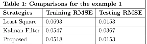
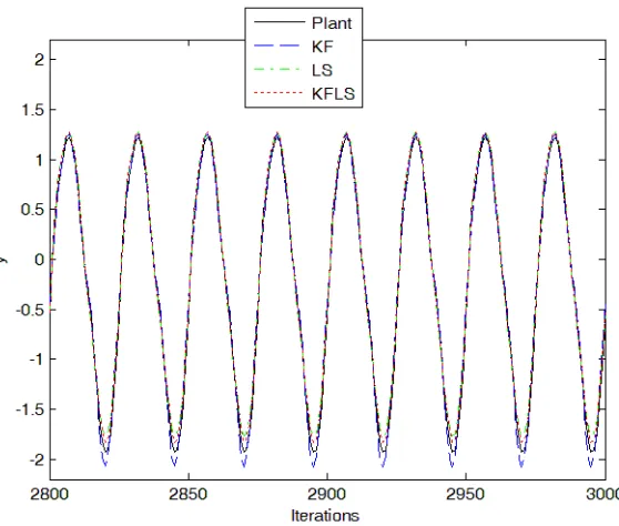
Figures 3, 4, and 5 show the comparisons for the norm of the gain (_kGkk), the training,

and testing of the Least Square, Kalman Filter, and Proposed. The training and testing RMSE comparisons of (31) are shown in Table 1.

Table 1: Comparisons for the example 1

Strategies Training RMSE Testing RMSE

Least Square 0:0693 0:0153

Kalman Filter 0:0547 0:0367

Proposed 0:0518 0:0153

Figure 3: Norm of the gain for the example 1

Figure 5: Testing for the example 1

4.2

Example 2

The complex process of the example 2 is detailed as follows [27]:

y(k) = 0:3y(k 1) + 0:6y(k 2) +f(u(k 1)) (33)

with

f(u(k 1)) = 0:6 sin( u(k 1)) + 0:3 sin(3 u(k 1)) + 0:1 sin(5 u(k 1))

u(k 1) = sin 2 (k 1) 200

The complex process of equations (1), (33) where inputs are x1(k) = y(k 1), x2(k) =

y(k 2), x3(k) = u(k 1)and the output isy(k) = y(k). The data of 3000iterations is used

for the training and the data of the least 200 iterations is used for the testing.

The Least Square of [25] is detailed as (2), (3), (4) with elements N = 3, M = 5, g1 = 1 103, r2 = 0:2, bvj(1) and wbj(1) employ random numbers between0 and 1.

The Kalman Filter of [26] is detailed as (2), (3), (5) with elements N = 3, M = 5, g1 = 1 103, r1 = 1 10 1, r2 = 0:2, bvj(1) and wbj(1) employ random numbers between 0

The Proposed algorithm is detailed as (2), (3), (6), (7) with elements N = 3, M = 5, g1 = 1 103, r1 = 1 10 1, r2 = 0:2, bvj(1) and wbj(1) employ random numbers between 0

and 1.

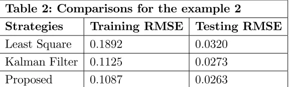
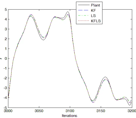
Figures 6, 7, and 8 show the comparisons for the norm of the gain (_kGkk), the training,

and testing of the Least Square, Kalman Filter, and Proposed. The training and testing RMSE comparisons of (31) are shown in Table 2.

Figure 6: Norm of the gain for the example 2

Table 2: Comparisons for the example 2

Strategies Training RMSE Testing RMSE

Least Square 0:1892 0:0320

Kalman Filter 0:1125 0:0273

Proposed 0:1087 0:0263

Figure 7: Training for the example 2

is smaller for the …rst. Thus,the Proposed is the best option for the modeling in the example 2.

5

Conclusion

In this research, a novel algorithm was introduced for the updating of a neural network. The stability and convergence of the gain in the proposed algorithm were assured by the Lyapunov technique. From examples, it was seen that the proposed algorithm achieves better accuracy when compared with both the recursive least square algorithm and extended Kalman …lter for the modeling of two complex processes. The proposed algorithm could be used to train a fuzzy system, or it could be used as the updating of an evolving intelligent system. In the future research, the proposed method will be used for the control, pattern recognition, prediction, or classi…cation.

6

Acknowledgements

Authors are grateful to the editors and the reviewers for their valuable comments. Authors thank the Secretaría de Investigación y Posgrado, the Comisión de Operación y Fomento de Actividades Académicas del Instituto Politécnico Nacional, and Consejo Nacional de Ciencia y Tecnología for their help in this research. The second author acknowledges the support of the Austrian COMET-K2 programme of the Linz Center of Mechatronics (LCM), funded by the Austrian federal government and the federal state of Upper Austria. This publication re‡ects only the authors views.

References

[1] A. Y. Alanis, L. J. Ricalde, C. Simetti, F. Odone, Neural model with particle swarm optimization Kalman learning for forecasting in smart grids, Mathematical Problems in Engineering, 2013 (2013) 1-9.

[2] A. Y. Alanis, E. N. Sanchez, A. G. Loukianov, Discrete-time recurrent neural induc-tion motor control using Kalman learning, Internainduc-tional Joint Conference on Neural Networks, (2006) 1993-2000.

[4] K. J. Astrom, B. Wittenmark, Adaptive Control - Second Edition, Addison-Wesley Longman Publishing Co., Inc., Boston, MA, USA, (1994).

[5] A. Bifet, R. Gavalda, Kalman …lters and adaptive windows for learning in data streams, L. Todorovski, N. Lavrac, K. P. Jantke, Discovery Science, Lecture Notes in Computer Science, 4265 (2006), 29-40, Springer, Berlin Heidelberg.

[6] S. Celikovsky, Topological equivalence and topological linearization of controlled dy-namical systems, Kybernetika, 31 (1995) 141-150.

[7] G. Chen, Q. Xie, L. S. Shieh, Fuzzy Kalman …ltering, Journal of Information Sciences, 109 (1998) 197-209.

[8] J. K. Coelho, M. D. Pena, O. J. Romero, Pore-scale modeling of oil mobilization trapped in a square cavity, IEEE Latin America Transactions, 14 (4) (2016) 1800-1807.

[9] Z. Deng, X. Wang, Y. Hong, Distributed optimisation design with triggers for disturbed continuous-time multi-agent systems, IET Control Theory and Applications, 11 (2) (2017) 282-290.

[10] K. Dolinsky, S. Celikovsky, Kalman …lter under nonlinear system transformations, American Control Conference, (2012) 4789-4794.

[11] S. M. Guo, L. S. Shieh, G. Chen, N. P. Coleman, Observer-type Kalman innovation …lter for uncertain linear systems, IEEE Transactions on Aerospace and Eelectronic Systems, 37 (4) (2001) 1406-1418.

[12] J. E.Guillermo, L. J. Ricalde Castellanos, E. N. Sanchez, A. Y. Alanis, Detection of heart murmurs based on radial wavelet neural network with Kalman learning, Neuro-computing, 164 (2015) 307-317.

[13] E. A. Hernandez-Vargas, P. Colaneri, R. H. Middleton, Switching Strategies to Mitigate HIV Mutation, IEEE Transactions on Control Systems Technology, 22 (4) (2014) 1623-1628.

[14] E. A. Hernandez-Vargas, P. Colaneri, R. H. Middleton, Optimal therapy scheduling for a simpli…ed HIV infection model, Automatica, 49 (2013) 2874-2880.

[16] R. Khemchandani, A. Pal, S. Chandra, Fuzzy least squares twin support vector clus-tering, Neural Computing and Applications, (2016). DOI: 10.1007/s00521-016-2468-4

[17] L. Ljung, System Identi…cation: Theory for the User, Prentice Hall PTR, Prentic Hall Inc., Upper Saddle River, New Jersey, (1999).

[18] E. Lughofer, Evolving Fuzzy Systems - Methodologies, Advanced Concepts and Appli-cations, (2011), Springer, Berlin Heidelberg.

[19] E. Lughofer, Single-Pass Active Learning with Con‡ict and Ignorance, Evolving Sys-tems, 3 (4) (2012) 251-271.

[20] E. Lughofer, E. Weigl, W. Heidl, C. Eitzinger, T. Radauer, Recognizing input space and target concept drifts in data streams with scarcely labeled and unlabelled instances, Information Sciences, 355-356 (2016) 127-151.

[21] I. Mansouri, A. Gholampour, O. Kisi, T. Ozbakkaloglu, Evaluation of peak and residual conditions of actively con…ned concrete using neuro-fuzzy and neural computing tech-niques, Neural Computing and Applications, (2016). DOI: 10.1007/s00521-016-2492-4

[22] V. K. Nguyen, F. Klawonn, R. Mikolajczyk, E. A. Hernandez-Vargas, Analysis of prac-tical identi…ability of a viral infection model, Plos one, (2016) 1-16.

[23] M. Pratama, J. Lu, S. Anavatti, E. Lughofer, C. P. Lim, An incremental meta-cognitive-based sca¤olding fuzzy neural network, Neurocomputing, 171 (2016) 89-105.

[24] B. Rehaka, S. Celikovsky, Numerical method for the solution of the regulator equation with application to nonlinear tracking, Automatica, 44 (2008) 1358-1365.

[25] J. J. Rubio, Least square neural network model of the crude oil blending process, Neural Networks, 78 (2016) 88-96.

[26] J. J. Rubio, W. Yu, Nonlinear system identi…cation with recurrent neural networks and dead-zone Kalman …lter algorithm, Neurocomputing, 70 (13) (2007) 2460-2466.

[27] J. J. Rubio, SOFMLS: Online self-organizing fuzzy modi…ed least square network, IEEE Transactions on Fuzzy Systems, 17 (6) (2009) 1296-1309.

[29] X. M. Sun, X. F. Wang, Y. Hong, W. Xia, Stabilization control design with parallel-triggering mechanism, IEEE Transactions on Industrial Electronics, (2016). DOI: 10.1109/TIE.2016.2637888

[30] Z. Weng, G. Chen, L. S. Shieh, J. Larsson, Evolutionary programming Kalman …lter, Information Sciences, 129 (2000) 197-210.