A Model for the Mass Growth of Wild Caught Fish

ISSN Online: 2327-4026 ISSN Print: 2327-4018

DOI: 10.4236/ojmsi.2019.71002 Nov. 22, 2018 19 Open Journal of Modelling and Simulation

A Model for the Mass-Growth of Wild-Caught

Fish

Katharina Renner-Martin, Norbert Brunner, Manfred Kühleitner, Werner-Georg Nowak,

Klaus Scheicher

Institute of Mathematics, University of Natural Resources and Life Sciences, Vienna, Austria

Abstract

The paper searched for raw data about wild-caught fish, where a sigmoidal growth function described the mass growth significantly better than non-sigmoidal functions. Specifically, von Bertalanffy’s sigmoidal growth func-tion (metabolic exponent-pair a = 2/3, b = 1) was compared with unbounded linear growth and with bounded exponential growth using the Akaike informa-tion criterion. Thereby the maximum likelihood fits were compared, assuming a lognormal distribution of mass (i.e. a higher variance for heavier animals). Starting from 70+ size-at-age data, the paper focused on 15 data coming from large datasets. Of them, six data with 400 - 20,000 data-points were suitable for sigmoidal growth modeling. For these, a custom-made optimization tool iden-tified the best fitting growth function from the general von Bertalanffy-Pütter class of models. This class generalizes the well-known models of Verhulst (lo-gistic growth), Gompertz and von Bertalanffy. Whereas the best-fitting models varied widely, their exponent-pairs displayed a remarkable pattern, as their dif-ference was close to 1/3 (example: von Bertalanffy exponent-pair). This defined a new class of models, for which the paper provided a biological motivation that relates growth to food consumption.

Keywords

Growth Models Described by the von Bertalanffy-Pütter Differential Equation, Model Selection Using the Akaike Information Criterion, Maximum Likelihood Fit Based on a Lognormal Distribution of Mass, Optimization Using Simulated Annealing

1. Introduction

1.1. Growth Models

Size-at-age (length or mass) is an important metric about animals and so there is How to cite this paper: Renner-Martin, K.,

Brunner, N., Kühleitner, M., Nowak, W.-G. and Scheicher, K. (2019) A Model for the Mass-Growth of Wild-Caught Fish. Open Journal of Modelling and Simulation, 7, 19-40.

https://doi.org/10.4236/ojmsi.2019.71002

Received: October 22, 2018 Accepted: November 19, 2018 Published: November 22, 2018

Copyright © 2019 by authors and Scientific Research Publishing Inc. This work is licensed under the Creative Commons Attribution International License (CC BY 4.0).

DOI: 10.4236/ojmsi.2019.71002 20 Open Journal of Modelling and Simulation a large body of literature about which growth models fit best to given size-at-age data. The von Bertalanffy [1] and Pütter [2] differential Equation (1) provides a comprehensive framework for the most common models for mass-growth:

( )

_{( )}

_{( )}

d d

a b

m t

p m t q m t

t = ⋅ − ⋅ (1)

It describes body mass m(t) > 0 as a function of age t, using the following five model parameters: The exponent-pair a < b (“metabolic scaling exponents”) and the constants p and q are assumed to be non-negative; m0 > 0 is an initial value, i.e.m(0) = m0. In the case of equal exponents, Equation (1) is replaced by the generalized Gompertz [3] differential Equation (2), the limiting case of Equation (1), when b approaches a:

( )

_{( )}

₍

_{( )}

₎

_{( )}

d

ln d

a a

m t

p m t q m t m t

t = ⋅ − ⋅ ⋅ (2)

This equation uses four model parameters: a, p, q (non-negative) and m0 > 0. In general, the solutions of (1) and (2) are expressed in terms of non-elementary functions, namely hypergeometric functions [4] and exponential integrals [5], respectively. The present paper used numerical solutions [6] [7]. For several “named models” these equations could be solved by elementary means, namely for the exponent-pairs a = 2/3 and b = 1 of von Bertalanffy [1], a = 3/4, b = 1 of West [8], a = 1, b = 2 for logistic growth of Verhulst [9], and a = b = 1 of Gom-pertz [3]. There are also elementary solutions for Richards’ [10] model (a = 1 and b > 1 is a free parameter) and for the generalized von Bertalanffy model (b = 1 and 0 ≤ a < 1 is a free parameter). The von Bertalanffy growth function for length (VBGF) fits to the present framework, too: It is a special case of Equation (1) using the exponent pair a = 0, b = 1 (bounded exponential growth). Other special cases are power-laws between mass and time (q = 0, p > 0), in particular linear growth (a = b = q = 0, p > 0, m0 > 0).

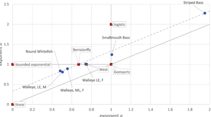
Figure 1 plots the exponent-pairs for these named models. Several of these

models were motivated by competing biological theories about the relation be-tween growth and metabolism; whereby different authors proposed different exponent-pairs [11]. However, these models “have only a loose connection to the biology behind the actual growth processes” [12]. Therefore, no single growth model may be exactly correct for all species [13]. For fish, in particular, the op-timal parameters of the growth models may depend on environmental factors

[14] [15]. Where there is no information about other biological factors for

growth, the models may nevertheless be used to extract relevant information from the data, as is current practice fisheries management [16].

1.2. Shape of the Growth Curves

DOI: 10.4236/ojmsi.2019.71002 21 Open Journal of Modelling and Simulation

Figure 1. Exponent-pairs of named models and optimal fits. Red squares indicate named models, grey lines indicate more general model classes, and blue dots indicate best fitting models to the in-dicated data. The dashed grey line indicates a new model class of this paper.

growth curves (solutions of the model equations) are increasing, bounded and sigmoidal (S-shaped): Initially the rate of growth increases, until the inception point is reached. Subsequently, it decreases to zero in the limit, when the asymptotic mass (mmax) is reached. The latter condition (m' = 0) provides the following equation for the asymptotic mass:

1

max for ,

b a p

m a b

q −

 

=_{ } <

  and max exp for

p

m a b

q  

= _{ } =

  (3)

The parameters a, b, p, q come from Equation (1) and Equation (2), respec-tively. For exceptional exponents and parameters, the growth curves may be non-sigmoidal (a = 0) or unbounded (p > 0, q = 0). For instance, the most common growth model in fisheries literature, VBGF for length (Google search for “VBGF, fish”: ca. 15,000 results), is not sigmoidal. However, it is equivalent to a sigmoidal model for mass-growth in the following sense [1]: If length-growth follows VBGF, and if mass is assumed to be proportional to a power Lk _{of length} L (k > 1), then mass-growth is described by the exponent-pair a = 1 − 1/k > 0, b

= 1 (sigmoidal growth curve).

DOI: 10.4236/ojmsi.2019.71002 22 Open Journal of Modelling and Simulation exponent was acceptable, too. As the authors noted, such a high variability has implications for data-fitting, as standard search strategies may not always find the right direction towards the optimum parameters, if there is no significant difference in the fits. Indeed, fisheries management literature reported problems with convergence [18]. The authors attributed the high variability of the expo-nents to differences in data quality, as most non-fish data were average values from controlled studies, where measurements were conducted repeatedly for the same group of animals, while most fish-data were about wild-caught fish, where each fish contributed only once in its lifetime to the measurements. Such data were also affected by gear-selectivity, where there may be few data about young (small) fish, as these could escape from the trawler nets, or as anglers preferred to harvest large fish, and few data about older fish, as most of them did not sur-vive long enough to come close to their maximum size, resulting in many dif-ferent possible shapes for the catch-curve that describes the age structure of the collected data [19]. As a consequence, several data supported unbounded growth

[20]; [21] reported this for about 1/3 of their fish data. This was considered as an

indication for too few data about older animals. By similar considerations, where data supported bounded non-sigmoidal growth this was considered as an indi-cation for too few data about young fish.

1.3. Problem of the Paper

The conclusion about the high variability for fish-data was drawn from da-ta-fitting to average weights. The present paper therefore reconsidered this issue and asked, if data-fitting to raw data would change the picture. More specifically, the paper aimed at identifying data that could be fitted well by a bounded sig-moidal mass-growth curve and where this fit was clearly superior to the fit by typically non-sigmoidal model functions. These data were deemed insofar as suitable for the application of sigmoidal growth models, as the variability of the exponents was more restricted.

To achieve this goal, the paper compared the fit of three typical models: Linear growth, as it represents unbounded models, bounded exponential growth, as it represents bounded non-sigmoidal models, and the von Bertalanffy expo-nent-pair, as it represents sigmoidal growth. This comparison was applied to various data for wild-caught fish, whereby the model curves were fitted to the raw data from [22]. Further, data-fitting took into account the typically heteros-cedastic distributions of size (meaning a larger variance for a higher mass). The paper tested, if there was an acceptable fit by the sigmoidal model, but no ac-ceptable fit by the other two models. The paper then explored, based on this test, how many of the considered catch data were suitable for the application of sig-moidal growth functions. For these data it determined the best fitting sigsig-moidal model amongst models described by Equation (1) and Equation (2) and searched for a pattern of the optimal exponent-pairs.

Me-DOI: 10.4236/ojmsi.2019.71002 23 Open Journal of Modelling and Simulation thods. For instance, a visual inspection alone did not suffice to recognize that the fit of the bounded exponential model was acceptable for Figure 2, but not ac-ceptable for Figure 3, when compared to the von Bertalanffy exponent-pair model. For, the plot did not reveal, for how many data-points a good/poor fit was achieved.

2. Methods

2.1. Materials

The authors conducted a literature search for growth data of wild-caught fish, referring to the following secondary sources: 39 data-sets came from a repository by Derek Ogle [22] listed under “growth” (Table 1 for the file names). The con-version of length-at-age data into mass-at-age was based on Fish Base [23]. All data were processed in Mathematica 11.3 of Wolfram Research_{; Appendix} ex-plains the used code. As it is generally accepted in fisheries research that model comparison is a data-hungry exercise, only data for population-level studies with initially at least 500 data-points (different fish) were considered. Further, data were removed if after the elimination of incomplete data-points (e.g. size at an unknown age) and filtering (e.g. by sex) there remained fewer than about 100 data-points or less than six points of time (The former condition was not strict, but the latter was, as the paper compared models with up to 6 free parameters).

2.2. Data Fitting

Literature in fisheries management prefers to fit model curves directly to the raw data, assuming a heteroscedastic distribution of size. Most common is the as-sumption of a lognormal distribution [24], as by Equation (4) for a lognormal distribution the standard deviation stdev of size is proportional to the expected

Figure 2. Mass-at-age data (blue), geometric mean (green), and growth curves, based on data #02 about Cabezon with length converted into mass. Parameters of the growth curves were: dashed a = b = q = 0, m0 = 1766.7, p = 870.4; black a = 2/3, b = 1, m0 =

DOI: 10.4236/ojmsi.2019.71002 24 Open Journal of Modelling and Simulation

Figure 3. Mass-at-age data (blue), geometric mean (green), and four growth curves, based on data #11 (male Walleye from Lake Erie). The parameters of the growth curves were: dashed curve a = b = q = 0, m0 = 199.7, p = 242.1; black a = 2/3, b = 1, m0 = 151.6, p

= 12.97, q = 1.03; red a = 0, b = 1, m0 = 73.3, p = 384.95, q = 0.15; blue = best fit: a =

0.463, b = 0.884, m0 = 120.742, p = 38.483, q = 1.529.

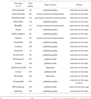
Table 1. Type of the original sources and processing of 39 data-sets.

File name

in [22] points Data Type of source Actiona AHerringChile 121 published graphic removed: too few data AnchovetaChile 207 private, personal communication removed: too few data BlackDrum2001 141 government, personal communication removed: too few data BlueCatfish 119 published graphic removed: too few data BluegillIL 61 private, personal communication removed: not size at age

Bonito 253 published graphic removed: too few data BullTroutRML2 96 published graphic removed: too few data Cabezon 525 private, personal communication selected: retrieved #2 CreekChub 218 published graphic removed: too few data

Croaker2 318 published graphic removed: too few data DarterOnt 54 published graphic removed: too few data EuroPerchTJ 69 published graphic removed: too few data FWDrumLE1 1577 published table selected: retrieved #3

Jonubi1 410 published table removed: too few data LakeTroutALTER 86 Repository removed: too few data LJCisco 378 published table removed: too few data Morwong4 392 Repository removed: too few data

Mosquitofish 9127 published graphic removed: too few ages _{(3 years)}

DOI: 10.4236/ojmsi.2019.71002 25 Open Journal of Modelling and Simulation

Continued

RockBassLO1 1288 published table selected: retrieved #7

RuffeSLRH92 739 government, personal communication removed: too few ages _{(4 years)}

RWhitefishAI 995 published table selected: retrieved #8 RWhitefishIR 103 published table removed: too few data

SardineChile 196 private, personal communication removed: too few data SardineLK 75 published graphic removed: too few data SculpinALTER 117 repository removed: too few data SiscowetMI2004 780 government, personal communication selected: retrieved #4 - 5

SMBassWB 445 repository selected: retrieved #9 SpottedSucker1 96 secondary source removed: too few data

SpotVA1 403 report removed: too few data StripedBass2 1201 report selected: retrieved #10

TroutBR 851 report selected: retrieved #1 and #6 TroutperchLM1 431 published table removed: too few data

WalleyeErie2 33,734 government, personal communication selected: retrieved #11 - 12 WalleyeML 14,583 government, personal communication selected: retrieved #13 - 14 WalleyeRL 1543 published table selected: retrieved #15 WhiteGrunt2 465 published graphic removed: too few data YERockfish 159 private, personal communication removed: too few data

a_{#n is the numbering of the data that were retrieved from the selected dataset.}

value ev of size with the shape parameter as (approximate) constant of propor-tionality:

2 exp

2

s ev= _m+ _

  and

(

( )

)

2

2

exp 1

2 s

stdev ev= ⋅ _ _− ≈ev s O s⋅ +

  (4)

Here, m is the location parameter and s > 0 is the shape parameter of a log-normal distribution and the rightmost term in Equation (4) assumes s ≈ ₀

(whe-reby O(∙) refers to the Taylor series remainder). The present paper used this ap-proach in order to conform to established practice in fisheries management lite-rature (A different approach assumes a normal distribution for each age class, but an age dependent variance; e.g. [25]).

DOI: 10.4236/ojmsi.2019.71002 26 Open Journal of Modelling and Simulation

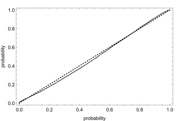
Figure 4. Probability plot. The figure assesses the fit of a normal distribution (location parameter m = 0, shape parameter s = 0.241) with the differences of the logarithm of mass and the respective age-class averages of the logarithm of mass for the data of Figure 3. The dotted line is the diagonal and the solid line is the P-P-plot, which compares the normal distribution (x-axis) with the observed cumulative distribution function (whereby a good fit is indicated by closeness to the diagonal).

2.3. Optimization

There are several approaches for heteroscedastic data fitting, amongst them weighted least-squares for the mass-at-age data, using the reciprocals of the standard deviations (of mass at each age class) as weights. The present paper uses instead transformed data. For, technically data-fitting to lognormally dis-tributed mass-at-age data (i.e. maximum likelihood estimation of the optimal distribution and growth function parameters) is equivalent to using a logarith-mic transformation of mass and the method of least squares to fit the trans-formed growth function u(t) = ln(m(t)) to these transformed data (Thereby also the parameters for linear growth, m = m0 + p⋅t, were determined from a nonli-near regression for u).

Further, (for the transformed data) the least squares method is equivalent to the minimization of the lack-of-fit sum of squares LFSS, where LFSS is the weighted sum of the deviations of the model curve from the averages at each age (the weight is the count of data at this age). The present paper used this refor-mulation of the least squares method to speed up computations (It has been used earlier in fisheries management, e.g. [27]). The use of LFSS has the following justification: The method of least squares assumes that the errors (deviations from the model curve) are random, meaning independent (normally distributed) random variables with expected value 0. Therefore, the sum of the squared er-rors, SSE, may be decomposed into SSE = LFSS + PESS, where PESS, the sum of squares of pure errors, is the sum of the squared deviations of the data at each age from the averages at each age. Curve fitting can only minimize LFSS, while

DOI: 10.4236/ojmsi.2019.71002 27 Open Journal of Modelling and Simulation Summarizing, data fitting was reduced to minimizing LFSS, a weighted sum of the squared differences between the average of the logarithmic weights at this age and the logarithm of the growth curve at this age.

The data fit to the three test models (linear, bounded exponential, and von Bertalanffy exponent-pair) used the Mathematica function NMinimize and si-mulated annealing [28] as optimization method. Further, the parameters of the bounded models were restricted so as to ensure an “empirically meaningful” asymptotic mass, defined from a comparison of the asymptotic mass mmax of Equation (3) with the maximal (arithmetic) mean value of the mass at different ages. If mmax was in the interval between half and twice that maximal average mass, as could be observed e.g. for the model curves in Figure 3, then the cor-responding model curve was accepted as empirically meaningful. This constraint helped to avoid that optimization was trapped at clearly false growth functions (e.g. constant functions). Note that the paper did not simplify optimization by using literature values for the initial condition m0 (e.g. natal mass) or for the asymptotic mass mmax.

For the subsequent optimization of the general models (1) and (2), the paper used a custom-made variant of simulated annealing to minimize LFSS, but without constraints. This approach is explained below for the search of the pa-rameters for the general von Bertalanffy-Pütter model (1). The following com-putations were repeated in a loop of 500,000 steps. Using starting values for the parameters a, b, m0, p, q (starting from the optimal parameters of the von Berta-lanffy exponent-pair or, Equation (2), from random numbers), it multiplied them by random numbers between 1 ±_{dist, but close to 1 (e.g. dist = 0.01); this}

deviated from the usual simulated annealing, where small random numbers are added. If the altered parameters improved LFSS, they were accepted. Otherwise, the increase of ln(LFSS/N) was compared with an exponentially distributed random number (e.g. mean value exm = 1; N = number of data points); this function was motivated by Akaike’s [29] index explained below. If the increase was below this random number, the altered parameters were accepted. Other-wise, the previous parameters were retained. The parameters dist and exm were set by the authors so as to obtain a reasonable convergence (several experments). After each 10,000 steps, dist and exm were reset: They were reduced by 10% in order to avoid moving too fast too far away from a good candidate for the opti-mum and the computations were restarted with the best hitherto found parame-ters. For several data the loop was repeated. In case that the optimal exponents were close to the diagonal (distance below 0.1), the optimization was repeated for the generalized Gompertz Equation (2). For the present data this did not oc-cur. For three data the custom-made optimization approach was needed also for the von Bertalanffy exponent-pair, as the general purpose procedures produced a stack-overflow.

2.4. Model Selection

DOI: 10.4236/ojmsi.2019.71002 28 Open Journal of Modelling and Simulation motivated by the Akaike information criterion [29], namely the following pseu-do-Akaike-weight pprob defined from a pseudo-Akaike index PAIC. In terms of this index, the most acceptable model has the least PAIC, defined below. The best fitting model (least LFSS) needs not be most acceptable (penalty for addi-tional parameters).

(

)

(

)

(

)

LFSS K K

PAIC AC K

N AC K

⋅ ⋅ +

 

= ⋅  + ⋅ + _{− −}

  (5)

The relation of formula (4) to the usual AIC is explained below. PAIC was de-fined from the lack-of-fit sum of squares for the model, LFSS (model), from the number N of data-points, from the number AC of age classes and from the number K of optimized parameters. Thereby, K = 4 for the test models (except for linear growth: K = 3), as m0, p, q and implicitly the shape parameter s of the lognormal distribution were optimized. Further, K = 5 and K = 6 for the genera-lized Gompertz model (2) and the von Bertalanffy-Pütter model (2), respectively. The index pprob compares a given model with the most acceptable one.

(

)

e pprob

e −∆

−∆

=

+ (6) Here, ∆ _{= PAIC (model) – PAIC (most acceptable model) > 0. The paper}

de-fined a fit as acceptable, if pprob ≥ 2.5%. As the maximal value is pprob = 50%, inacceptable fits were linked to the lowest 5% of possible values of pprob. For example, in Figure 3 and Figure 2 the von Bertalanffy exponent-pair model had the best fit amongst the three compared models. For Figure 3, but not for

Fig-ure 2, the fit was insofar significantly better, as none (respectively both) of the

non-sigmoidal models had an acceptable fit. Further, for both figures the best fitting model (amongst those considered) did not reduce LFSS enough to mi-nimize also pprob. Thus, its predictive power was highest amongst the consi-dered models, but the loss in simplicity may not have been justified by the gain in predictive power.

The following outline explains, why the authors decided to use pprob as a measure of the goodness of fit. PAIC is a modification of the Akaike index AICc for small samples [30] [31]; for variants c.f. [32]. Recall AICc = N∙ln(SSE/N) + 2∙K + 2∙K∙(K + 1)/(N −_K − _{1); in this formula the authors replaced N by AC and}

SSE by LFSS⋅_{AC/N. Thus, PAIC assessed the fit of the models in terms of their}

fit to the averages (of the logarithmically transformed data) at age, weighted by the percentage of data represented by this age. Therefore, pprob was the Akaike weight relative to this fit to averages.

DOI: 10.4236/ojmsi.2019.71002 29 Open Journal of Modelling and Simulation model with more parameters is not deemed as better, unless the number of age classes is high enough to support more parameters. Further, the Akaike meas-ures depend heavily on the assumption of normally distributed data, which is not exactly true for all fish data, as was noted previously. By contrast, for (weighted) averages of large samples (of logarithmically transformed mass) there is a theoretical justification for assuming a normal distribution, whence for

PAIC and pprob the usual interpretations for the Akaike index and the Akaike weight may be assumed. In particular, pprob may be interpreted as a probability that a model is true, assuming that one of the considered models is true. In view of this interpretation, pprob has the same meaning, independently of the consi-dered data, whence it could be used to define the notion of an acceptable fit.

3. Results

The authors screened 39 datasets from the repository [22]. As Table 1 explains, two datasets were removed as they did not inform about size-at-age, 24 were removed, as they informed about less than 500 fish, and two were removed, as they informed about only 3 - 4 years of growth. For datasets with 400 - 500 fish inclusion was reconsidered; a dataset from an internet repository was included. 31% of datasets were retrieved from published graphics, 26% came from person-al communications (from the government or a private data collector), 23% came from published tables that used only a mild aggregation (e.g. counting fish for each possible length-age class), 10% came from internet repositories, 8% from locally distributed reports, and one from another secondary source. The selec-tion process was not uniform over the sources; local reports and government communications met the selection criteria best (about 2/3 of them were selected) and published graphics worst (all removed by lack of data or ages).

The finally retained 11 datasets could be further split by species and by gend-er, resulting in 15 fish data (Table 2). They inform #1 about Brown Trout ( Sal-mo trutta); #2 about Cabezon (Scorpaenichthys marmoratus); #3 about Fresh-water Drum (Aplodinotus grunniens); #4 - 5 about Lake Trout (Salvelinus na-maycush) of the Siscowet strain; #6 about Rainbow Trout (Oncorhynchus my-kiss); #7 about Rock Bass (Ambloplites rupestris); #8 about Round Whitefish (Prosopiumcylindraceum); #9 about Smallmouth Bass (Micropterusdolomieu); #10 about Striped Bass (Moronesaxatilis); and #11 - 15 about Walleye (Sander vitreus).

The authors did not aim at including data retrieved from diagrams. For, when retrieving data from diagrams, then the information about multiplicity is lost. For example, digitalizing Figure 3 could (at best) identify 6489 different da-ta-points but it could not discern the 13,677 duplicates (67.8% of the data).

Fig-ure 5 illustrates that the duplicates were not distributed uniformly across all age

DOI: 10.4236/ojmsi.2019.71002 30 Open Journal of Modelling and Simulation

Table 2. Characteristics of the data.

No. Locationa _Sexb _{Data Duplicates Size}c _{Ages Conversion}d _{of L in M}

#1 Bois Brule River U 224 84.8% inch 7 0.01127 × (L × 2.54)2.96

#2 Oregon Coast F 299 62.2% cm 13 0.02914 × L3

#3 Lake Erie U 1577 60.6% mm 13 0.0483 × (L/10)3

#4

Lake Superior M 94 34.0% gram 10 none #5 F 104 29.8% gram 15

#6 Bois Brule River U 627 90.3% inch 8 0.0101 × (L × 2.54)3.063

#7 Lake Ontario U 1288 72.7% mm 9 0.0314 × (L/10)2.923

#8 Lake Superior U 995 77.0% inch 9 0.00885 × (L × 2.54)3.223

#9 West Bearskin Lake U 445 35.5% mm 11 0.00469 × (L/10)3.2

#10 Atlantic coast U 1201 84.4% inch 18 0.00945 × (L × 2.54)2.907

#11

Lake Erie M 20,166 67.8% gram 20 none #12 F 13,155 60.9% gram 17

#13

Mills Lacs Lake M 6414 88.2% mm 17

0.02914 × (L/10)3.008

#14 F 8169 88.5% mm 16

#15 Red Lakes U 1543 64.2% mm 6

a_{Locations from the USA;} b_{F female, M male, U unsexed;} c_{Size at age in years;} d_{Conversion into gram.}

Figure 5. Catch curve for data #11 of Figure 3 (male Walleye from Lake Erie, USA) based on (a) all data and (b) data without duplicates (lower bars). The figure counts, how many fish were observed for each age-class.

DOI: 10.4236/ojmsi.2019.71002 31 Open Journal of Modelling and Simulation fitting using the raw data. However, as averages (arithmetic means) may differ significantly from geometric means (Figure 6), data of the form average size and count at age were not considered, either.

Table 3 and Figure 1 summarize the results of data fitting. All data were

plotted to check their plausibility (For one dataset, paste & copy changed age 10 to age 1 generating a U-shaped growth curve; this was then corrected). All data had between 30% - 90% duplicates (Table 2). For two of the 15 selected data, the bounded linear growth had the best fit (least LFSS); for eight it had an acceptable fit (pprob ≥ 2.5%). Further, for eight data linear growth had an acceptable fit. Thus, for six (ca. 2/3) of data the fit by the representative for sigmoidal growth was not significantly more acceptable than the fit by the (simpler) non-sigmoidal models, whence it was considered to be futile to seek the best fitting sigmoidal model. Data quality appeared to matter insofar, as the percentage of data that were suitable for fitting sigmoidal growth models was higher for data with 16 or more ages (c.f. Table 2). This was insofar plausible, as many species of fish con-tinue to grow over many years. Further, for the 15 selected data there was a sig-nificantly positive correlation coefficient (0.69) between the number of data-points and the number of ages (t-test at 99.5% significance), which was plausible, too.

Six data were identified as suitable for sigmoidal growth. For these, the optim-al exponent-pairs (fit of the generoptim-al von Bertoptim-alanffy-Pütter model) were com-puted (Table 4). Figure 1 plots the location of the optimal exponent-pairs in re-lation to the traditional named models with assumed exponent pairs. Apparent-ly, the optimal exponent-pairs were unrelated to any model or model class (ex-cept for one Walleye close to the West model). All exponent-pairs were remote from the Gompertz-class (diagonal a = b), from the non-sigmoidal class (a = 0 and b > 0) and (except for Smallmouth Bass) from Richards’ model (a = 1 and

b > 1). In comparison, the exponent-pairs seemed to be close to the generalized von Bertalanffy models (b = 1 and a < 1), but for the two species (Bass) the ex-ponent a > 1 was incompatible with this model class. Also the distances between

DOI: 10.4236/ojmsi.2019.71002 32 Open Journal of Modelling and Simulation

Table 3. Comparison of three models to test the sigmoidal shape of the data.

No

LFSS pprob

Sigmoidala

Linear _exponential Bounded _{Bertalanffy Linear} Von _Exponential Bounded _Bertalanffy Von

1 0.995 1.17 0.506 50% 0% 1% N 2 0.727 0.818 0.566 50% 5% 36.7% N 3 63.9 64.75 46.47 50% 9.5% 47.57% N 4 0.693 0.636 0.61 50% 7.1% 8.6% N 5 2.202 1.906 1.714 50% 30.5% 49.3% N 6 7.468 1.427 1.033 3.7% 21.5% 50% N 7 14.031 13.24 12.7584 50% 3.4% 4.0% N 8 24.607 36.756 1.269 0% 0% 50% Y 9 63.792 66.611 3.804 0% 0% 50% Y 10 40.605 46.562 13.889 0% 0% 50% Y 11 192.21 28.72 16.94 0% 0.5% 50% Y 12 99.09 122.54 10.38 0% 0% 50% Y 13 170.79 3.81 8.55 0% 50% 0.1% N 14 73.1 32.95 19.43 0% 1.4% 50% Y 15 23.12 1.94 15.84 50% 0% 0% N

a_{Y yes, N no.}

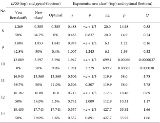
Table 4. Comparison of three models for optimality.

No

LFSS (top) and pprob (bottom) Exponents: new classa _{(top) and optimal (bottom)}

Von

Bertalanffy classNew a _Optimal a b m0 p Q

8 1.269 0.385 0.385 0.488 =a + 1/3 20.0 14.98 0.88 50% 34.7% 0% 0.483 0.837 20.0 14.9 0.74

9 3.804 1.853 1.841 0.973 =a + 1/3 6.1 1.22 0.16 42.8% 50% 0.4% 1.007 1.243 6.1 1.36 0.32

10 13.889 3.597 3.596 1.947 =a + 1/3 699.1 0.00066 0.0000037 0% 50% 9.0% 1.951 2.279 699.7 0.00065 0.000038

11 16.943 13.560 13.560 0.506 =a + 1/3 119.9 38.0 3.78 39.7% 50% 11.0% 0.506 0.807 119.9 38.0 3.78

12 10.382 10.08 10.0 0.713 =a + 1/3 112.3 10.48 0.69 50% 14.0% 1.5% 0.742 1.009 112.9 10.31 1.17

14 19.433 17.741 17.741 0.557 =a + 1/3 427.7 33.92 1.66 50% 19.0% 1.6% 0.557 0.891 427.7 33.92 1.66

a_{The “new class” refers to the Parks-1/3 model explained in the Discussion section.}

mi-DOI: 10.4236/ojmsi.2019.71002 33 Open Journal of Modelling and Simulation nimal LFSS) may extend over a wide region; the authors [34] observed this also in a different context (least squares approximation to average size at age data). Further, Figure 1 displayed a pattern for the approximate location of the optim-al exponent-pairs. They were close to the dashed line b = a + 1/3, even for large values of the exponents. Thereby 1/3 was not the optimal difference between the exponents, but it was chosen, as it defines a new model class introduced in this paper. The Discussion will provide a biological interpretation for the difference

d = b – a of the exponents, based on an alternative explanation of Equation (1).

4. Discussion and Conclusion

4.1. The Parks—1/3 Model Class

The traditional explanation of differential Equation (1) proposed that the rate of growth would be proportional to the difference between anabolism and catabol-ism, both of which would be proportional to a power of mass. Specific values of the exponents were then derived from biophysical arguments; e.g.: b = 1, as ca-tabolism would be proportional to mass (number of sustained cells) and a = 2/3, as anabolism would be proportional to the gills’ surface (oxygen consumption) and therefore to the 2/3th _{power of mass [1].}

The present alternative explanation of Equation (1) hypothesizes that body mass would be a function of the total food intake F(t) since birth (t = 0), where-by the (individual) asymptotic mass mmax would be approached at a rate depen-dent on instantaneous food intake:

( )

max d

d

d d

d d

F k

t

m m

m t

t = ⋅

− (7)

In the formula, k1 > 0 a constant of proportionality and d is a constant that explains the speed of growth: With the same total food intake F, with a larger d

the asymptotic mass mmax is approached faster. This model, using d = 1, was proposed by Parks ([35] at p. 26), who supported it by evidence from farmed animals. The food consumption, which cannot be observed for wild-caught fish, can be eliminated by the additional hypothesis that the instantaneous food in-take dF/dt would be proportional to the energy needs E (i.e. dF/dt = k2∙E), which in turn would be proportional to a power of body mass (i.e.E = k3∙ma). Substi-tuting this into Equation (7), then after a multiplication and renaming of con-stants (p = k1∙k2∙k3∙(mmax)d, q = k1∙k2∙k3) this simplifies to Equation (8), which is just another parametrization of Equation (1):

( )

_{( )}

_{( )}

d d

a a d

m t

p m t q m t

t

+

= ⋅ − ⋅ (8)

spe-DOI: 10.4236/ojmsi.2019.71002 34 Open Journal of Modelling and Simulation cial cases. As the von Bertalanffy exponent-pair is a special case of the Parks-1/3 model class, the present paper investigates this class.

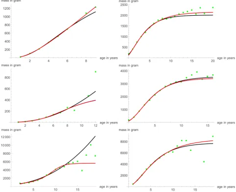
Figure 1 suggests that the Parks-1/3 model class may come close to providing

the best-fitting description of the mass-growth of several species of fish. Figure 7

illustrates the good fit compared to the best-fitting and the von Bertalanffy mod-els for the six considered data. The optimization used the custom-made ap-proach, starting with a, m0, p, q of the optimal model (setting b = a + 1/3). Table

4 summarizes the outcome of the data-fit for this model class. In comparison to the von Bertalanffy exponent-pair model and the best fitting von Bertalanf-fy-Pütter model, the Parks-1/3 model had the most acceptable fit for three data and an acceptable fit for the three other data, where the von Bertalanffy expo-nent-pair model had the most acceptable fit. However, the fit of the von Berta-lanffy exponent-pair model was not acceptable for data #10 (It was acceptable,

DOI: 10.4236/ojmsi.2019.71002 35 Open Journal of Modelling and Simulation when compared with the non-sigmoidal models, but the consideration of the best-fitting model changed the assessment). Further, the fit of the Parks-1/3 model was nearly optimal, as seen in Figure 7: For all data the Parks-1/3 curve coincided with the best-fitting von Bertalanffy-Pütter curve. Consequently, the Parks-1/3 model was more acceptable, as it used fewer parameters.

4.2. Conclusions

There were surprisingly few data that supported the hypothesis of a sigmoidal shape of mass growth, and those did support the new Parks-1/3 model (expo-nent-pairs b = a + 1/3).

The 39 datasets allowed to define 70+ data using additional stratifications. When testing the suitability of these data for modeling sigmoidal growth, more than 3/4 of these data were removed due to poor data quality (insufficient size). Of the remaining 15 data almost 2/3 were removed due to the insufficient fit of a sigmoidal growth function. A speculative explanation for the insufficient fit may be data quality, again. There were some data with notable differences between the arithmetic and geometric mean (Figure 6). This difference was caused by the presence of atypically small fish. In case that this difference has a biological meaning (e.g. slow and fast growth as different survival strategies), then it may be meaningful to split the data and model the growth of slow and of fast growing fish separately.

For all six data that were suitable for modeling sigmoidal growth, the Parks-1/3 model provided an acceptable fit; for 50% of the data it improved upon the von Bertalanffy exponent-pair model (one significant improvement) despite the penalty for the additional free parameter. Therefore, when compared to the model classes of Richards, Gompertz or the generalized von Bertalanffy model, the Parks-1/3 model may provide the most realistic description of the mass growth of fish. In particular, the advantage of this model is its considera-tion food consumpconsidera-tion and the flexibility gained by an addiconsidera-tional parameter that for all data resulted in a near optimal fit.

Conflicts of Interest

The authors declare no conflicts of interest regarding the publication of this pa-per.

References

[1] Bertalanffy, L.V. (1957) Quantitative Laws in Metabolism and Growth. Quarterly Reviews of Biology, 32, 217-231.https://doi.org/10.1086/401873

[2] Pütter, A. (1920) Studien über physiologische Ähnlichkeit. VI. Wachstumsähnlichkeiten.

Pflügers Archiv für die Gesamte Physiologie des Menschen und der Tiere, 180, 298-340. https://doi.org/10.1007/BF01755094

DOI: 10.4236/ojmsi.2019.71002 36 Open Journal of Modelling and Simulation

[4] Ohnishi, S., Yamakawa, T. and Akamine, T. (2014) On the Analytical Solution for the Pütter-Bertalanffy Growth Equation. Journal of Theoretical Biology, 343, 174-177.https://doi.org/10.1016/j.jtbi.2013.10.017

[5] Marusic, M. and Bajzer, Z. (1993) Generalized Two-Parameter Equations of Growth. Journal of Mathematical Analysis and Applications, 179, 446-462.

https://doi.org/10.1006/jmaa.1993.1361

[6] Burden, R.L. and Faires, J.D. (1993) Numerical Analysis, PWS Publishing Co., Bos-ton, MA.

[7] Leader, J.J. (2004) Numerical Analysis and Scientific Computation. Addi-son-Wesley, Boston.https://doi.org/10.1038/35098076

[8] West, G.B., Brown, J.H. and Enquist, B.J. (2001) A General Model for Ontogenetic Growth. Nature, 413, 628-631.

[9] Verhulst, P.F. (1838) Notice sur la loi que la population suit dans son accroissement. Correspondence Mathematique et Physique (Ghent), 10, 113-121. [10] Richards, F.J. (1959) A Flexible Growth Function for Empirical Use. Journal of

Ex-perimental Botany, 10, 290-300.https://doi.org/10.1093/jxb/10.2.290

[11] Isaac, N.J.B. and Carbone, C. (2010) Why Are Metabolic Scaling Exponents So Controversial? Quantifying Variance and Testing Hypotheses. Ecology Letters, 13, 728-735.https://doi.org/10.1111/j.1461-0248.2010.01461.x

[12] Enberg, K., Dunlop, E.S. and Jørgensen, C. (2008) Fish Growth. In: Jørgensen, S.E. and Fath, B.D., Eds., Encyclopedia of Ecology, Elsevier, Oxford, 1564-1572.

https://doi.org/10.1016/B978-008045405-4.00205-6

[13] White, C.R. (2010) Physiology: There Is No Single p. Nature, 464, 691-693.

https://doi.org/10.1038/464691a

[14] Killen, S.S., Atkinson, D. and Glazier, D.S. (2010) The Intraspecific Scaling of Me-tabolic Rate with Body Mass in Fishes Depends on Lifestyle and Temperature.

Ecology Letters, 13, 184-193.https://doi.org/10.1111/j.1461-0248.2009.01415.x

[15] Yamamoto, Y. and Kao, S.J. (2012) Relationship between Latitude and Growth of Bluegill Lepomis macrochirus in Lake Biwa, Japan. Annales Zoologici Fennici, 49, 36-44.https://doi.org/10.5735/086.049.0104

[16] Ogle, D. and Iserman, D.A. (2017) Estimating Age at a Specified Length from the von Bertalanffy Growth Function. North American Journal of Fisheries Manage-ment, 37, 1176-1180.https://doi.org/10.1080/02755947.2017.1342725

[17] Renner-Martin, K., Brunner, N., Kühleitner, M., Nowak, W.G. and Scheicher, K. (2018) On the Exponent in the Von Bertalanffy Growth Model. PeerJ, 6, e4205.

https://doi.org/10.7717/peerj.4205

[18] Shi, P.-J., Ishikawa, T., Sandhu, H.S., Hui, C., Chakraborty, A., Jin, X.-S., Tachihara, K. and Li, B.-L. (2014) On the 3/4-Exponent van Von Bertalanffy Equation for On-togenetic Growth. Ecological Modelling, 276, 23-28.

https://doi.org/10.1016/j.ecolmodel.2013.12.020

[19] Sukhanov, V.V. (2016) Age-Distribution Models for Fish in Catches. Russian Jour-nal of Marine Biology, 42, 111-116. https://doi.org/10.1134/S1063074016020115

[20] Apostolidis, C. and Stergiou, K.I. (2014) Estimation of Growth Parameters from Published Data for Several Mediterranean Fishes. Journal of Applied Ichthyology, 30, 189-194.https://doi.org/10.1111/jai.12303

DOI: 10.4236/ojmsi.2019.71002 37 Open Journal of Modelling and Simulation

[22] Ogle, D. (2018) R for Fisheries Analysis.

[23] Froese, R. and Pauly, D. (2018) FishBase Data Base. http://www.fishbase.org [24] Manabe, A., Yamakawa, T., Ohnishi, S., Akamine, T., Narimatsu, Y., Tanaka, H.,

Funamoto, T., Ueda, Y. and Yamamoto, T. (2018) A Novel Growth Function In-corporating the Effects of Reproductive Energy Allocation. PLoS ONE, 13, e0199346. https://doi.org/10.1371/journal.pone.0199346

[25] Wilson, K.L., Matthias, B.G., Barbour, A.B., Ahrens, R.N.M., Tuten, T. and Allen, M.S. (2015) Combining Samples from Multiple Gears Helps to Avoid Fishy Growth Curves. North American Journal of Fisheries Management, 35, 1121-1131.

https://doi.org/10.1080/02755947.2015.1079573

[26] Evans, D.L., Drew, J.H. and Leemis, L.M. (2017) The Distribution of the Kolmogo-rov-Smirnov, Cramer-von Mises, and Anderson-Darling Test Statistics for Expo-nential Populations with Estimated Parameters. In: Glen, A.G. and Leemis, L.M., Eds., Computational Probability Applications, Springer International Publishing, New York, 165-190.

[27] Gutreuter, S. and Krzoska, D.J. (1994) Quantifying Precision of in Situ Length and Weight Measurements of Fish. North American Journal of Fisheries Management, 14, 318-322. https://doi.org/10.1577/1548-8675(1994)014<0318:QPOISL>2.3.CO;2

[28] Vidal, R.V.V. (1993) Applied Simulated Annealing. Lecture Notes in Economics and Mathematical Systems. Springer-Verlag, Berlin.

https://doi.org/10.1007/978-3-642-46787-5

[29] Akaike, H. (1974) A New Look at the Statistical Model Identification. IEEE Trans-actions of Automatic Control, 19, 716-723.

https://doi.org/10.1109/TAC.1974.1100705

[30] Burnham, K.P. and Anderson, D.R. (2002) Model Selection and Multi-Model Infe-rence: A Practical Information-Theoretic Approach. Springer, Berlin.

[31] Motulsky, H. and Christopoulos, A. (2003) Fitting Models to Biological Data Using Linear and Nonlinear Regression: A Practical Guide to Curve Fitting. Oxford Uni-versity Press, Oxford.

[32] Dziak, J.J., Coffman, D.L., Lanza, S.T. and Li, R. (2017) Sensitivity and Specificity of Information Criteria. PeerJ Preprints, 5, e1103v3.

https://doi.org/10.7287/peerj.preprints.1103v3

[33] Mackay, D. and Moreau, J. (1990) A Note on the Inverse Function of the von Berta-lanffy Growth Function. Fishbyte, 8, 29-31.

[34] Renner-Martin, K., Brunner, N., Kühleitner, M., Nowak, W.G. and Scheicher, K. (2018) Optimal Exponent-Pairs for the Von Bertalanffy-Pütter Growth Model.

PeerJ Preprints, 6, e27152v1.https://doi.org/10.7287/peerj.preprints.27152v1

DOI: 10.4236/ojmsi.2019.71002 38 Open Journal of Modelling and Simulation

Appendix: Annotated Mathematica Code

Data were imported from sheet n of an Excel file, sorted (lexicographically) and the title line was dropped:

dat1 = Import[“C:\\...\\filename.xlsx”]; dataraw = Sort[Drop[dat1[[n]], 1]]; Authors first checked the size (minimum about 100), the percentage of dupli-cates (minimum about 30% to remove data retrieved from diagrams) and the number of ages (minimum 6). Further, authors plotted the catch curve to check for irregularities.

Length[dataraw];

1-Length[Union[dataraw]]/Length[dataraw];

Length[GatherBy[dataraw, First]];counts = Tally[Transpose[rawdata][[1]]]; chartcounts =

BarChart[Apply[Labeled, Reverse[counts, 2], {1}], AxesLabel -> {“age”, “count”}]

Several data were length-at-age, using different units (inch, cm, mm); these were converted into mass (in g) at age, using literature values (FishBase for total length in cm in g). Further, the range of the data (minimal and maximal ages and masses) was checked and the arithmetic mean of mass at age together with its maximum value (for assessing empirical meaningfulness) was evaluated.

datamass = Map[{#[[1]], cona*(#[[2]]*conunits)^conb} &, dataraw]

/. {conunits -> unit conversion, cona -> literature value, conb -> literature value};

sort = Sort[datamass];

{timemin, timemax, weightmin, weightmax} =

{Min[Transpose[sort][[1]]], Max[Transpose[sort][[1]]], Min[Transpose[sort][[2]]], Max[Transpose[sort][[2]]]} // N;

gdata = GatherBy[sort, First]; avarith = Map[Mean, gdata] // N;

gweightmax = Max[Transpose[avarith][[2]]];

In order to prepare the best fit, a logarithmic transformation was applied to the mass data. Further, the geometric means at each age were evaluated and plotted together with the mass-at-age data.

logdata = Map[{#[[1]], Log[#[[2]]]} &, sort]; ldata = GatherBy[logdata, First];

avlog = Map[Mean, ldata] // N;

avgeo = Map[{#[[1]], Exp[#[[2]]]} &, avlog]; dataplot =

ListPlot[{sort, avgeo},

PlotStyle -> {{PointSize[0.01], Blue}, {PointSize[0.015], Green}}, AxesLabel -> {“age in years”, “mass in gram”}, PlotRange -> All, PlotLegends -> {“data”, “geometric mean”}];

de-DOI: 10.4236/ojmsi.2019.71002 39 Open Journal of Modelling and Simulation fines these as numeric variables). This function was defined from using a nu-meric solution f = sol of the differential Equation (1); thereby the Block-method was used to define local variables:

ssr[a_?NumberQ, b_?NumberQ, c_?NumberQ, p_?NumberQ, q_?NumberQ] := Block[{sol, f},

sol = NDSolve[{f'[t] == p*f[t]^a - q*f[t]^b, f[timemin] == c}, f, {t, timemin, timemax}][[1]];

Sum[counts[[n, 2]]*(Log[f[avlog[[n, 1]]] /. sol] - avlog[[n, 2]])^2, {n, 1, Length[avlog]}]];

The subsequent optimization using Simulated Annealing was conducted by the same scheme for each test model: linear growth, sigmoidal von Bertalanffy growth, non-sigmoidal bounded growth. For linear growth, the constraints m0 > 0 for the initial value and p > 0 for the rate of increase were added. For the other growth functions these constraints were restricted further: The initial value was constrained to exceed 10% of the least observed mass and the parameter q was constrained so as to ensure an empirically meaningful asymptotic mass. Further, the optimal growth curves, the data and the geometric means were plotted and finally LFSS was compared:

optlin =

NMinimize[{ssr[0, 0, c, p, 0], c > 0, p > 0}, {c, p}, Method -> “SimulatedAn-nealing”];

optbert = NMinimize[{ssr[2/3, 1, c, p, q], c > weightmin/10, p > 0, q > p/(2*gweightmax^(1/3)), q < p/(0.5*gweightmax^(1/3))}, {c, p, q}, Method -> “SimulatedAnnealing”];

optexp = NMinimize[{ssr[0, 1, c, p, q], c > weightmin/10, p > 0, q > p/(2*gweightmax), q < p/(0.5*gweightmax)}, {c, p, q}, Method -> “SimulatedAnnealing”];

lin = f /. NDSolve[{f'[t] == p, f[timemin] == c} /. optlin[[2]], f, {t, timemin, timemax}][[1]];

linplot = Plot[lin[x], {x, timemin, timemax}, PlotStyle -> Dashed];

bert = f /. NDSolve[{f'[t] == p*f[t]^(2/3) - q*f[t], f[timemin] == c} /. opt-bert[[2]], f, {t, timemin, timemax}][[1]];

bertplot = Plot[bert[x], {x, timemin, timemax}, PlotStyle -> Black]; exp = f /. NDSolve[{f'[t] == p - q*f[t], f[timemin] == c} /. optexp[[2]], f, {t, timemin, timemax}][[1]];

explot = Plot[exp[\[FormalX]], {\[FormalX], timemin, timemax}, PlotStyle -> Red];

Show[{ListPlot[sort, PlotStyle -> {PointSize[0.01], Blue}],

ListPlot[avgeo, PlotStyle -> {PointSize[0.015], Green}], linplot, explot, bertplot},

DOI: 10.4236/ojmsi.2019.71002 40 Open Journal of Modelling and Simulation paic[sse_?NumberQ, n_?IntegerQ, m_?IntegerQ, k_?IntegerQ] :=

m*Log[sse/n] + 2*k + 2*k*(k + 1)/(m - k - 1);

probaic[x_, y_] = Exp[-(x - y)/2]/(1 + Exp[-(x - y)/2]); pseudoaics =

{paic[lfsslin, Length[sort], Length[counts], 3], paic[lfssexp, Length[sort], Length[counts], 4], paic[lfssbert, Length[sort], Length[counts], 4]}; minaic = Min[pseudoaics];

pprob =

{probaic[pseudoaics[[1]], minaic], probaic[pseudoaics[[2]], minaic], probaic[pseudoaics[[3]], minaic]};

The custom-made simulated annealing started with the optimal parameters for the Von Bertalanffy exponent-pair model and followed the procedures ex-plained in text, whereby the logarithm of LFSS was optimized. Also this optimal growth function was plotted.

{a0, b0, c0, p0, q0} = {2/3, 1, c, p, q} /. optbert[[2]]; sse = ssr[a0, b0, c0, p0, q0]; llh = - Log[sse];

{ssemin, amin, bmin, cmin, pmin, qmin} = {sse, a0, b0, c0, p0, q0}; \[Alpha] = 1.0; s = 0.01;

Do[

If[Mod[i, 10000] == 0, \[Alpha] *= 0.9; Print[i, “ ”, \[Alpha] s];

{sse, a, b, c, p, q} = {ssemin, amin, bmin, cmin, pmin, qmin}];

{ac, bc, cc, pc, qc} = RandomReal[{1 - \[Alpha]*s, 1 + \[Alpha]*s}, 5] {a, b, c, p, q};

ssec = ssr[ac, bc, cc, pc, qc]; llhc = -Log[ssec];

If[Log[RandomReal[]] < (llhc - llh)/\[Alpha], {a, b, c, p, q} = {ac, bc, cc, pc, qc}];

sse = ssec; llh = llhc; If[sse < ssemin,

Print[i, “ ”, {ssemin, amin, bmin, cmin, pmin, qmin} = {sse, a, b, c, p, q}]], {i, 500000}]

puett =

f /. NDSolve[{f'[t] == pmin*f[t]^amin - qmin*f[t]^bmin, f[timemin] == cmin}, f,

{t, timemin, timemax}][[1]];