Gender based Segregation before and after the Great Recession

Munich Personal RePEc Archive

Gender-based Segregation before and

after the Great Recession

Humpert, Stephan

Leuphana University

2015

Online at

https://mpra.ub.uni-muenchen.de/63555/

Gender-based Segregation before and after the Great Recession

Stephan Humpert

BAMF, Frankensstr. 210, 90461 Nuremberg / Germany

dr.stephan.humpert(at)bamf.bund.de

&

Leuphana University Lueneburg, Scharnhorststr.1, 21335 Lueneburg / Germany

humpert(at)leuphana.de

ABSTRACT

Pooled international survey data is used to analyze occupational

segregation in times of the great recession. Observing over 30 European

economies and the United States over a time span of 10 years, I present

evidence of a somehow surprising crisis effect on gender-based

segregation. While all economies differ in their general magnitudes, the

economic downturn affects a temporary reduction of segregation in

terms of two dissimilarity measures.

Keywords: Gender Segregation, Duncan Index, Karmel-MacLachlan Index, European

Social Survey (ESS), General Social Survey (GSS)

1. Introduction:

The economic crisis of 2007/2008 hit economies world-wide and especially there labor

markets. In this paper I analyze the topic from a view of gender equality. Therefore, I

use pooled European Social Survey data (ESS) and, U.S. General Social Survey (GSS)

with the time span 2002 to 2012, to calculate two measures of gender-specific

segregation (Duncan and Karmel-MacLachlan). The effect of the economic crisis is

visible in most observed economies. Here, between 2008 and 2010, those economies

have a temporary reduction of their segregation magnitudes. This somehow surprising

result is driven by a redistribution of the male-female employment ratio. While males

work more often in cyclic or export-orientated occupations and industries, they suffer

more from job-losses than females. Sierminska and Takhtamanova (2011) call the

phenomenon of higher job separation and lower job finding rates of male workers

‘mancession’. Figure 1 shows that males have in general higher employment rates in the

decade of observation (EU and U.S), but perceive a higher reduction in times of the

crisis, as well.

This descriptive paper is structured as following. In section two we give a brief review

of the literature. In the section three I describe both data sets and the methodology. The

results are reported and discussed in section four, while I give a brief conclusion in the

Figure 1 – Gender-specific employment-rates (EU without Croatia and U.S.)

Source: Labour Force Survey, Eurostat (2014)

2. Literature review:

Following the definition of Alonso-Villar and del Rio (2014) I understand segregation

as a non-similar distribution of a specific sub-population over organizational units. Here

females can be over or under-represented over a set of given occupations relative to

males. It is well known that men and women differ in their occupations. This

phenomenon is known as horizontal segregation, while vertical segregation denotes the

over or under-represented of a group at the top of a given occupation (e.g. Estévez-Abe

2006).

A series of papers verify the incident of gender-based segregation over time and space.

E.g. Blau and Hendricks (1979), Charles (1992), Hakim (1992), Anker (1997), Baunach

(2002), Estévez-Abe (2006), Jarman et al. (2012), Schäfer et. al (2012), Lippa et al.

(2014), and Humpert (2014a) show world-wide cross-country evidence for occupational

2002 2003 2004 2005 2006 2007 2008 2009 2010 2011 2012 50

55 60 65 70 75 80

segregation. One finding is that segregation decline over time. However, Blau et al.

(2013), and Humpert (2014b) show that different coding of job classifications have an

impact on the calculation of segregation measures.

3. Data and Methodology:

For the analysis two social surveys, the European Social Survey (ESS) data with pooled

information for 32 economies for six waves of observations each (2002 to 2012). In this

data, 24 countries are members of the EU, while the others are not. The U.S. General

Social Survey (GSS) include a much longer time span from 1972 to 2012. But for the

case of the analysis it is shortened to the same waves. Both are weighted with obligatory

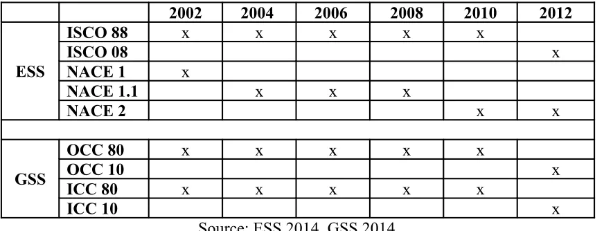
sample weights taken from by the data provider. Table 1 provides a matrix of given

years, and characteristics. For the descriptive analysis I analyze occupation-specific

segregation for man and women. This is made by two different segregation measures,

which are discussed below.

Table 1 - Time and classifications

2002 2004 2006 2008 2010 2012

ESS

ISCO 88 x x x x x

ISCO 08 x

NACE 1 x

NACE 1.1 x x x

NACE 2 x x

GSS

OCC 80 x x x x x

OCC 10 x

ICC 80 x x x x x

ICC 10 x

Here, occupations in the ESS data are measured by ISCO classifications (International

Standard Classification of Occupations) 1988 and 2008, while they are measured by

ICC (U.S. Census Occupational Coding) 1980 and 2010.

Unfortunately, not every classification is available for every economy and every year.

So structural breaks between two classifications, and cyclical differences in segregation

over time, may harm the power of the analysis. E.g. Humpert (2014b) for a discussion

of ISCO classifications and segregation over time. Here, the choice of a given ISCO

classifications has an effect on the intensity of segregation in a given year. The always

most actual classification available turns segregation into a relative stability (Humpert

2014a). For robustness reasons the same approach is conducted for industries, classified

by NACE groups (Nomenclature Générale des Activités Economique dans l'Union

Européenne) and CIC (U.S. Census Industry Coding).

For the analysis itself I calculate two general measures of segregation: the Duncan

index, and the Karmel-MacLachlan index. The Stata routine and the algebraic

description is given by Gradín (2014). I begin with a given population of N workers

distributed across T>1 organizational units with N=Σj=1 T

n_j>0

;nj 0_{being the total}

number of individuals in the jth occupation j=





partition of the population into two groups, males and females. Each group has size,

where i 0 j

n _{is the number of members of the ith group}





2 1 N + N =

N . In the first step, I use the Duncan index composed by Duncan and

Duncan (1955) to compute overall segregation. See equation (1) for the formula of the

D index.









/ /

1 2Σ /

1 = n N n N

= n n

In the second step the same approach is calculated with the Karmel-MacLachlan, or KM

index composed by Karmel and MacLachlan (1988). See equation (2) for the formula.







 



/ /

2 N N N N D n n

= n n

KM (2)

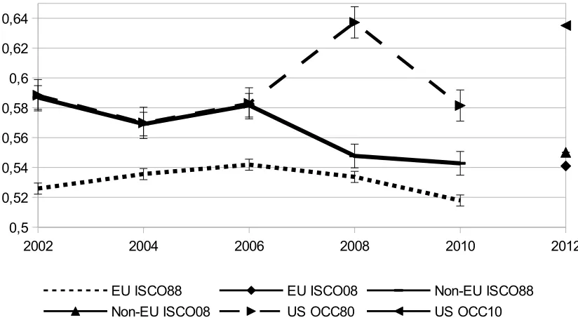
4. Results:

In this section I present computed results of the two indexes, and how segregation has

developed over time, especially in times of the crisis. For the purpose of simplicity I

present two figures, with pooled information for EU and non-EU economies taken from

the ESS and for the U.S. taken from the GSS. They represent occupation-specific

segregation. While figure 2 shows the computed results for the Duncan indices, figure 3

shows the values for the Karmel-McLachlin indices.

At first, economies with EU-member status are less segregated, than non-EU

economies. The lowest levels are in 2008 each. Here segregation declines from the

highest value in 2006 (EU: 0.5419, non-EU: 0.5817) to 2008 (EU: 0.5179, non-EU:

0.5428). In general, EU-members differ around 0.02 segregation points over time, while

the others differ around 0.04 segregation points. While both values for 2012 re-increase,

the EU-specific one raises more intensive. However, the 2012 value is calculated for

ISCO 2008 and not for ISCO 1988. Therefore, it is difficult to disentangle the increase

Figure 2 - Duncan Index (with standard errors)

Source: ESS 2014 and GSS 2014, own calculation with design weight.

Second, in U.S segregation is the highest, at all. Here, the values are even higher than

for the non-EU economies. In general, segregation in U.S. differs around 0.06

segregation points over time. The highest levels are in 2008 (0.6372), while the lowest

is in 2010 (0.5815). There is the interesting finding that non-EU and the U.S. are rather

identical between 2002 and 2006, while the scissor opens and the U.S. increases till

2008.

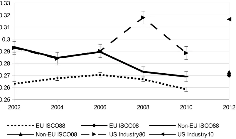
This pattern remains in terms of the Karmel-MacLachlan index, as well (figure 3). As

reported earlier, economies with EU-member status are lower segregated. The highest

levels are in 2006, and the lowest in 2010. This is the main differences between both

measures, that the lowest levels are calculated for 2008, or 2010. Here, segregation

declines from the highest value in 2006 (EU: 0.2704, non-EU: 0.2584) to 2010 (EU:

2002 2004 2006 2008 2010 2012

0,5 0,52 0,54 0,56 0,58 0,6 0,62 0,64

0.2894, non-EU: 0.2689). In general, EU-members differ around 0.01 segregation

points over time, while the others differ around 0.02 segregation points.

Again, U.S segregation remains the highest in this figure. In general, segregation in U.S.

differs around 0.03 segregation points over time. The highest levels are in 2008

(0.6372), while the lowest levels are in 2004 (0.2839) and 2010 (0.5815). As reported

above, the non-EU and the U.S. are rather identical between 2002 and 2006, while the

scissor opens and the U.S. increases till 2008.

Figure 3 - Karmel-MacLachlan Index (with standard errors)

Source: ESS 2014 and GSS 2014, own calculation with design weight.

The computed results for each of the economies are reported in tables 2 (ESS) and 3

(GSS) in the appendix-section. Generally spoken, each example of segregation shows a

generally declining trend. However, around the point of the Great Recession (2008 to

2010) the magnitudes decline very intensive, and turn back in 2012.

2002 2004 2006 2008 2010 2012

0,25 0,26 0,27 0,28 0,29 0,3 0,31 0,32 0,33

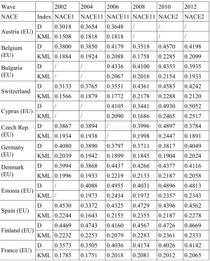
For robustness reasons the same approach is repeated for industry-specific segregation.

Here, NACE and ICC groups are used as substitutes of occupations. The crisis-specific

pattern remains with the described u-shape around the years 2008 to 2010. However,

three NACE and two ICC classifications do not fit in the timing of the ISCO or OCC

points of time. Therefore, the lowering of segregation is less easy to explain by the

effect of the economic downturn, or by changes in the industry-specific categories. See

tables 4 and 5 in the appendix-section for the country-specific results.

5. Conclusions:

To sum up, I use pooled European Social Survey data (ESS) for 32 European economies

and the U.S. General Social Survey (GSS) to analyze how gender-specific segregation

develop in times of the crisis. While I calculate the Duncan index, and the

Karmel-MacLachlan index for gender-specific differences in employment patterns, I present two

key results. First, EU member states in general are less segregated than the non-EU

ones. It is obvious that these economies are much more heterogeneous in their economic

power, and their national labor laws. However, it is clear that the U.S. is higher

segregated than the EU economy as a whole.

Second, there is a temporary effect of the economic crisis in most economies. Here,

between 2008 and 2010 economies realize a temporary reduction of segregation

magnitudes. The effect of lower segregation is based especially on male job-losses.

Males work more often in cyclical-sensitive occupations and industries, such as

construction. This follows the analysis of Maier (2011), who concludes that

employment is hit harder in every recession since the 1960s. However,

male-employment re-increases faster and higher in economic booms. On the other hand,

shrinks while males remain employed. However, the economic crisis itself hit all

workers notwithstanding being male or female. See for instance Gregory et al. (2013)

for a discussion of working time and work life balance in times of the recession.

Acknowledgment:

The findings, views, and conclusions expressed are entirely those of the author and

References:

Alonso-Villar, O., del Rio, C. (2014): Occupational Sex Segregation, In: Michalos, A.C.

(Ed.), Encyclopedia of Quality of Life and Well-Being Research, Berlin: Springer, pp.

4453-4456.

Anker, R. (1997): Theories of Occupational Segregation by Sex: An Overview,

International Labor Review, Vol. 136(3), pp. 315-339.

Baunach, D.M. (2002): Trends in Occupational Sex Segregation and Inequality, 1950 to

1990, Social Science Research, Vol. 31(1), pp. 77-98.

Blau, F.D., Hendricks, W.E. (1979): Occupational Segregation by Sex: Trends and

Prospects, Journal of Human Resources, Vol. 14(2), pp. 197-210.

Blau, F.D., Brummund, P., Liu, A.Y.-H. (2013): Trends in Occupational Segregation by

Gender 1970-2009: Adjusting for the Impact of Changes in the Occupational Coding

System, Demography, Vol. 50(2), pp. 471-492.

Charles, M. (1992): Cross-National Variation in Occupational Sex Segregation,

American Sociological Review, Vol. 57(4), pp. 483-502.

Duncan, O., Duncan, B. (1955): A Methodological Analysis of Segregation Indexes,

American Sociological Review, Vol. (20)2, pp. 210-217.

Estévez-Abe, M. (2006): Gendering the Varieties of Capitalism: A Study of

Occupational Segregation by Sex in Advanced Industrial Societies, World Politics, Vol.

59(1), pp. 142-175.

European Social Survey (ESS) (2014): ESS1- 6 cumulative data file, release date

Eurostat (2014): Labour Force Survey (annual average), release date October 22, 2014.

Gradín, C. (2014): Measuring Segregation using Stata: The two Group Case,

unpublished manuscript.

Gregory, A., Milner, S., Windebank, J. (2013): Work-life Balance in Times of

Economic Crisis and Austerity, International Journal of Sociology and Social Policy,

Vol. 33(9/10), pp. 528-541.

General Social Survey (GSS) (2014): GSS 1972-2012 Cross-Sectional Cumulative Data

release date June 19, 2014.

Hakim, C. (1992): Explaining Trends in Occupational Segregation: The Measurement,

Causes, and Consequences of the Sexual Division of Labour, European Sociological

Review, Vol. 8 (2), pp. 127-152.

Humpert, S. (2014a): Occupational Sex Segregation and Working Time: Regional

Evidence from Germany, Panoeconomicus, Vol. 61 (3), pp. 317-329.

Humpert, S. (2014b): Trends in occupational segregation: What happened with women

and foreigners in Germany?, European Economics Letters, Vol. 3(2), pp. 36-39.

Jarman, J., Blackburn R.M., Racko, G. (2012): The Dimensions of Occupational Gender

Segregation in Industrial Countries, Sociology, Vol. 46(6), pp. 1003-1019.

Karmel, T., MacLachlan, M. (1988): Occupational Sex Segregation - Increasing or

Decreasing, Economic Record, Vol. 64(3), pp. 147-179.

Lippa R.A., Preston K., Penner J. (2014): Women's Representation in 60 Occupations

from 1972 to 2010: More Women in High-Status Jobs, Few Women in Things-Oriented

Maier, F. (2011): Will the Crisis Change Gender Relations in Labour Markets and

Society?, Journal of Contemporary European Studies, Vol. 19(1), pp. 83-95.

Milkman, R. (1976): Women's Work and Economic Crisis: Some Lessons of the Great

Depression, Review of Radical Political Economics, Vol. 8(1), pp. 71-97.

Schäfer, A., Tucci, I., Gottschall, K. (2012): Top Down or Bottom Up? A

Cross-National Study of Vertical Occupational Sex Segregation in Twelve European

Countries, Comparative Social Research, Vol. 29, pp. 3-43.

Sierminska E., Takhtamanova Y. (2011): Job Flows, Demographics, and the Great

Recession, Research in Labor Economics, Vol. 32, pp. 115-154.

Watts, M. (1998): Occupational Gender Segregation: Index Measurement and

Appendix

Table 2 – Occupation-specific segregation (European Social Survey - ESS)

Wave 2002 2004 2006 2008 2010 2012

ISCO Class. Index ISCO 88 ISCO 88 ISCO 88 ISCO 88 ISCO 88 ISCO 08

Austria (EU) D 0.5254 0.5536 0.5520 / / / KML 0.2625 0.2754 0.2744 / / /

Belgium (EU)

D 0.5623 0.5941 0.6054 0.6317 0.6227 0.6162

KML 0.2784 0.2969 0.3024 0.3157 0.3113 0.3081

Bulgaria (EU)

D / / 0.6872 0.6595 0.6337 0.6371

KML / / 0.3298 0.3242 0.3135 0.3296

Switzerland D 0.5918 0.6065 0.6289 0.6677 0.6143 0.6223 KML 0.2959 0.3023 0.3135 0.3331 0.3068 0.3110

Cyprus (EU) D / / 0.6136 0.6164 0.6595 0.6321 KML / / 0.3065 0.3019 0.3298 0.3150

Czech Rep. (EU)

D 0.6117 0.6097 / 0.6222 0.6608 0.6068

KML 0.3058 0.3030 / 0.3111 0.3300 0.3032

Germany (EU)

D 0.6338 0.6224 0.6356 0.6096 0.6111 0.6257

KML 0.3167 0.3108 0.3178 0.3035 0.3049 0.3127

Denmark (EU)

D 0.6839 0.6348 0.6619 0.6478 0.6427 0.5824

KML 0.3417 0.3173 0.3309 0.3239 0.3210 0.2912

Estonia (EU) D / 0.6171 0.6826 0.6391 0.6594 0.7162 KML / 0.2979 0.3355 0.3119 0.3171 0.3489

Spain (EU) D 0.695 0.5815 0.6512 0.6299 0.5769 0.6192 KML 0.3270 0.2863 0.3246 0.3137 0.2869 0.3092

Finland (EU) D 0.6320 0.6658 0.6494 0.6336 0.6466 0.6598 KML 0.3158 0.3320 0.3246 0.3168 0.3229 0.3296

France (EU) D 0.6130 0.6099 0.6395 0.6145 0.5959 0.6037 KML 0.3062 0.3047 0.3197 0.3062 0.2976 0.3003

U.K. (EU) D 0.5847 0.6095 0.5878 0.5738 0.5683 0.6498 KML 0.2923 0.3047 0.2932 0.2864 0.2821 0.3187

Greece (EU) D 0.5385 0.5148 / 0.5296 0.5291 / KML 0.2683 0.2573 / 0.2645 0.2643 /

Croatia* D / / / 0.6276 0.5990 /

Hungary (EU)

D 0.6178 0.7069 0.6399 0.6895 0.5375 0.5948

KML 0.3088 0.3436 0.3131 0.3435 0.2923 0.2945

Ireland (EU) D 0.6480 0.6707 0.6567 0.6544 0.5806 0.6808 KML 0.3233 0.3317 0.3283 0.3268 0.2900 0.3402

Israel D 0.6271 / / 0.5852 0.6158 0.6002 KML 0.3128 / / 0.2910 0.3066 0.2982

Iceland D / 0.6138 / / / 0.6424

KML / 0.3063 / / / 0.3212

Italy (EU) D 0.6446 0.5978 / / / 0.6097 KML 0.3217 0.2892 / / / 0.3033

Lithuania (EU)

D / / / / 0.6909 0.7621

KML / / / / 0.3044 0.3745

Luxembourg (EU)

D 0.6780 0.6739 / / / /

KML 0.3390 0.3305 / / / /

Netherlands (EU)

D 0.6075 0.6220 0.6192 0.6150 0.5737 0.6156

KML 0.3023 0.3072 0.3094 0.3094 0.2864 0.3073

Norway D 0.6438 0.6130 0.6258 0.6182 0.5597 0.6309 KML 0.3215 0.3062 0.3127 0.3085 0.2799 0.3146

Poland (EU) D 0.6396 0.6445 0.6430 0.5918 0.5939 0.6514 KML 0.3198 0.3222 0.3211 0.2956 0.2969 0.3255

Portugal (EU)

D 0.6545 0.6170 0.6368 0.6104 0.6059 0.6791

KML 0.3267 0.3066 0.3131 0.3010 0.2970 0.3302

Russia D / / 0.6660 0.6781 0.6636 0.6976 KML / / 0.3250 0.3326 0.3260 0.3351

Sweden (EU) D 0.6449 0.6542 0.6199 0.6293 0.6332 0.6255 KML 0.3224 0.3270 0.3099 0.3146 0.3164 0.3124

Slovenia (EU)

D 0.6080 0.6510 0.6446 0.5446 0.6481 0.6480

KML 0.3040 0.3254 0.3224 0.2719 0.3236 0.3231

Slovakia (EU)

D / 0.6681 0.6655 0.6834 0.6363 0.6387

KML / 0.3339 0.3325 0.3303 0.3101 0.3136

Turkey D / 0.6478 / 0.5956 / /

KML / 0.2555 / 0.2310 / /

Table 3 – Occupation-specific segregation (General Social Survey - GSS)

Wave 2002 2004 2006 2008 2010 2012

US Census Index OCC80 OCC80 OCC80 OCC80 OCC80 OCC10

United States

D 0.5884 0.5699 0.5830 0.6372 0.5815 0.6351

KML 0.2928 0.2839 0.2901 0.3179 0.2885 0.3165

Source: GSS 2014, own calculation with design weight.

Table 4 – Industry-specific segregation (European Social Survey - ESS)

Wave 2002 2004 2006 2008 2010 2012

NACE Index NACE1 NACE11 NACE11 NACE11 NACE2 NACE2

Austria (EU) D 0.3018 0.3654 0.3648 / / / KML 0.1508 0.1818 0.1818 / / /

Belgium (EU)

D 0.3800 0.3850 0.4179 0.3518 0.4570 0.4198

KML 0.1884 0.1924 0.2088 0.1758 0.2285 0.2099

Bulgaria (EU)

D / / 0.4336 0.4100 0.4353 0.3935

KML / / 0.2067 0.2016 0.2154 0.1933

Switzerland D 0.3133 0.3765 0.3551 0.4361 0.4583 0.4242 KML 0.1566 0.1879 0.1772 0.2178 0.2288 0.2120

Cyprus (EU) D / / 0.4105 0.3441 0.4930 0.5052 KML / / 0.2090 0.1686 0.2465 0.2517

Czech Rep. (EU)

D 0.3867 0.3894 / 0.3996 0.4897 0.3784

KML 0.1934 0.1938 / 0.1998 0.2447 0.1891

Germany (EU)

D 0.4080 0.3890 0.3797 0.3711 0.3817 0.4049

KML 0.2039 0.1942 0.1899 0.1845 0.1904 0.2024

Denmark (EU)

D 0.3994 0.3868 0.4437 0.4266 0.4377 0.4116

KML 0.1996 0.1933 0.2219 0.2133 0.2187 0.2058

Estonia (EU) D / 0.4088 0.4955 0.4031 0.4896 0.4813 KML / 0.1973 0.2434 0.1972 0.2357 0.2343

Spain (EU) D 0.4530 0.3372 0.4325 0.4729 0.4396 0.4562 KML 0.2244 0.1643 0.2155 0.2355 0.2187 0.2278

Finland (EU) D 0.4469 0.4743 0.4160 0.4567 0.4726 0.4669 KML 0.2232 0.2253 0.2079 0.2283 0.2361 0.2333

U.K. (EU) D 0.3866 0.3907 0.4320 0.4062 0.4256 0.4191 KML 0.1932 0.1953 0.2155 0.2027 0.2113 0.2064

Greece (EU) D 0.3590 0.3390 / 0.3864 0.3860 / KML 0.1789 0.1695 / 0.1930 0.1928 /

Croatia* D / / / 0.4292 0.4987 /

KML / / / 0.2143 0.2493 /

Hungary (EU)

D / / 0.6399 0.4437 0.3926 0.4154

KML / / 0.3131 0.2209 0.1953 0.2060

Ireland (EU) D 0.4393 0.4577 0.4255 0.4926 0.4713 0.4862 KML 0.2192 0.2260 0.2127 0.2462 0.2355 0.2430

Israel D / / / 0.3218 0.4578 0.2977 KML / / / 0.1601 0.2278 0.1480

Iceland D / 0.4298 / / / 0.4677

KML / 0.2146 / / / 0.2338

Italy (EU) D 0.4025 0.3987 / / / 0.3788 KML 0.2009 0.1916 / / / 0.1882

Lithuania (EU)

D / / / / 0.3827 0.5400

KML / / / / 0.1667 0.2658

Luxembourg (EU)

D 0.4223 0.4677 / / / /

KML 0.2112 0.2290 / / / /

Netherlands (EU)

D 0.4027 0.4153 0.4064 0.3961 0.4012 0.4566

KML 0.2006 0.2050 0.2029 0.1980 0.2003 0.2279

Norway D 0.4701 0.4728 0.4678 0.4413 0.4250 0.4889 KML 0.2347 0.2361 0.2338 0.2202 0.2125 0.2443

Poland (EU) D 0.4179 0.4243 0.4331 0.3854 0.3956 0.4226 KML 0.2089 0.2121 0.2162 0.1926 0.1977 0.2111

Portugal (EU)

D 0.4709 0.4482 0.4963 0.4314 0.4872 0.5299

KML 0.2352 0.2229 0.2441 0.2126 0.2388 0.2579

Russia D / / 0.3861 0.4161 0.4846 0.4449 KML / / 0.1885 0.2041 0.2379 0.2127

Sweden (EU)

D 0.4973 0.4176 0.4392 0.4687 0.4725 0.4246

KML 0.2486 0.2087 0.2196 0.2343 0.2360 0.2120

Slovenia (EU)

D 0.3747 0.1658 0.4086 0.3297 0.4137 0.3988

KML 0.1873 0.0819 0.2038 0.1646 0.2066 0.1987

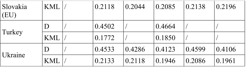
Slovakia (EU)

KML / 0.2118 0.2044 0.2085 0.2138 0.2196

Turkey D / 0.4502 / 0.4664 / /

KML / 0.1772 / 0.1850 / /

Ukraine D / 0.4533 0.4286 0.4123 0.4599 0.4106 KML / 0.2133 0.2118 0.1946 0.2086 0.1961 *Croatia joined the EU in 2014. Source: ESS 2014, own calculation with design weight.

Table 5 – Industry-specific segregation (General Social Survey - GSS)

Wave 2002 2004 2006 2008 2010 2012

US Census Index ICC80 ICC80 ICC80 ICC80 ICC80 ICC10

United States

D 0.4581 0.4844 0.4596 0.5402 0.5027 0.5060

KML 0.2279 0.2415 0.2286 0.2696 0.2491 0.2520