An Assessment of Case Based Reasoning for Spam Filtering

An Assessment of Case-Based Reasoning for

Spam Filtering

Sarah Jane Delany1_{, Pádraig Cunningham}2_{, Lorcan Coyle}2

1_{Dublin Institute of Technology, Kevin St., Dublin 8, Ireland.} [email protected] 2_{Trinity College Dublin, College Green, Dublin 2, Ireland.} {Padraig.Cunningham,Lorcan.Coyle}@tcd.ie

Abstract. Because of the changing nature of spam, a spam filtering system that uses machine learning will need to be dynamic. This suggests that a case-based (memory-based) approach may work well. Case-Based Reasoning (CBR) is a lazy approach to machine learning where induction is delayed to run time. This means that the case base can be updated continuously and new training data is immediately available to the induction process. In this paper we present a detailed description of such a system called ECUE and evaluate design decisions concerning the case representation. We compare its performance with an alternative system that uses Naïve Bayes (NB). We find that there is little to choose between the two alternatives in cross-validation tests on data sets. However, ECUE does appear to have some advantages in tracking concept drift over time.

1

Introduction

Spam classification is a challenging task for a number of reasons. Not least of these is the fact that something of an “arms race” has developed between spammers and the filtering systems developed to identify spam. The content and structure of spam messages is constantly changing as spammers attempt to bypass the techniques used by the filtering systems to catch the spam. This poses a difficult challenge as systems need to identify and learn new types of spam as this arms race continues.

Lazy learning is good for dynamically changing situations. With lazy learning the decision of how to generalise beyond the training data is deferred until each new unseen instance is considered. In comparison to this, eager learning systems determine their generalisation mechanism by building a model based on training data in advance of considering any new unseen instances. In this paper we present E-mail Classification Using Examples (ECUE), a lazy learning system using CBR that seamlessly incorporates new training data.

ECUE incorporates an effective case-based editing technique [1] which allows the number of training cases to remain at a manageable and efficient level.

The existing research on using a memory or case-based based approach [2,3] has a number of limitations. Firstly the evaluation is based on a restrictive data set incorporating legitimate email messages sent to a linguistics mailing list and “old-fashioned” spam emails that contain few of the obfuscations common in spam email today. Secondly all evaluations are static evaluations and do not take into account the changing nature of spam. In addition to static cross-validation tests, our evaluation of the approach presented in this paper includes dynamic evaluation of two independent datasets of over 10,000 email messages each received over the period of a year.

This paper begins with an overview of other work using machine learning techniques in spam filtering in Section 2. Section 3 presents ECUE, our case-based spam filtering approach and describes the feature selection, case retrieval and case-base management techniques we use. A preliminary evaluation of ECUE and comparison with NB is presented in Section 4. Section 5 outlines directions for future work while our conclusions are presented in Section 6.

2

Spam Filtering and Machine Learning

Existing research on using machine learning for spam filtering primarily uses NB as the technique of choice [2,4-6] with many unpublished implementations reported on the Web. In addition to NB there has been work using Support Vector Machines [7,8], Latent Semantic Indexing [9], and work using memory based classifiers [2,3,10]. Sakkis et al. [3] reported that their memory based classifier compared favourably to NB for spam filtering mailing lists and newsgroups while our preliminary findings [10] suggested that CBR would outperform NB.

Algorithms incorporating the NB classifier have proven to be among the most successful learners in the categorisation of text documents [11] and are good for high dimension data, hence their popularity in spam classification.

2.1 Naïve Bayes for Text Classification

NB is a probabilistic classifier that can handle a large number of features that other machine learning techniques cannot. It is ‘naïve’ in the sense that it assumes that the features are independent.

Consider a group of documents that are labelled as one of a set of classifications

ci∈ C. Each document is described by a set of attributes {a1,a2,…,an} where ai. indicates the presence of that attribute in the document. The classification returned from a NB classifier for a new document is given in Equation 1.

∏

∈

=

j j i

i C c

NB Pc Pa c

c

i

) | ( ) ( max

arg ₍₁₎

Due to the significance of false positives (legitimate emails identified incorrectly as spam) in spam filtering, the NB classifier is not generally used in this simple

argmax form. In practice the classification threshold is set to bias the classifier away from false positives (see Section 5.2).

njis the number of documents with classification cj. This provides a good estimate of the probability in many situations but in situations where nijis very small or even equal to zero this probability will dominate, resulting in an overall zero probability. A solution to this is to incorporate a small-sample correction into all probabilities called the Laplace correction [12]. The corrected probability estimate is given by Equation 2, where nki is the number of values for attribute ai. Kohavi et al. [13] suggest a value of f = 1/m where m is equal to the number of training documents.

) (

) ( ) |

(ai cj nij f nj f nki

P = + + × (2)

3

Case-Based Spam Filtering

This section describes ECUE, the case-based system we have implemented for spam filtering. The description includes details of the feature extraction and representation, feature selection, case retrieval and case-base editing techniques we have used.

3.1 Feature Extraction

In order to identify the possible lexical features from the training set of emails, each email was parsed and tokenised. No stop word removal, stemming or lemmatisation was performed on the text before tokenisation. Email attachments were removed before parsing but any HTML text present in the email was included in the tokenisation. The datasets used were personal datasets, i.e. all emails in each dataset were sent to the same individual. Hence it was felt that certain headers may contain useful information so a selection of header fields, including the Subject, To and From headers were included in the tokenisation.

Three types of features were identified:

• word features (i.e. sequences of characters separated by white space or separated by start and end HTML tag markers),

• letter or single character features,

• statistical features, e.g. the proportion of uppercase or lowercase characters.

No domain specific feature identification was performed at this stage although work by Sahami et al. [5] has indicated that the effectiveness of filters will be enhanced by their inclusion.

3.2 Feature Representation

For numeric features the standard way to determine the value of fi for feature xi is to use the normalised frequency fi,j of the feature, see Equation 3, where freqi,j is the number of times that feature xi occurs in email ej.

j l l

j i j

i

freq freq f

, , ,

max

= (3)

In the evaluation presented here we used this normalised frequency for word and letter features (separate normalisations for each type) and simply the proportion calculated for the statistical features (which is between 0 and 1 by definition).

A binary representation for the different types of feature is not so straightforward. For word features we use the simple existence rule that if the word exist in the email the feature value fi = 1 otherwise fi = 0. However for letter features, almost all letters or characters will occur within an email so using the existence rule is not useful. For letter features we use the Information Gain [14] value of the feature as calculated during the feature selection process (see Section 3.3) to determine whether to set

fi = 1. If the normalised frequency of the letter feature is greater than or equal to the normalised frequency which returns the highest information gain for that letter then the feature value is set to 1 in the case representation, otherwise it is zero. Given that statistical features are also values between 0 and 1, this rule was also applied to features of this type to determine their binary representation.

A series of experiments to evaluate whether features should be represented as binary or numeric features was performed (as discussed in Section 4.1). It is more normal in text classification for lexical features to carry frequency information but the results of our evaluations showed no significant improvements were demonstrated when using numeric features over binary features.

In addition using binary features allowed use of an efficient case retrieval algorithm (discussed in Section 3.4) to improve performance.

3.3 Feature Selection

Tokenising 1000 emails results in a very large number of features, (tens of thousands of features). Feature selection is necessary to reduce the dimensionality of the feature space. Yang and Petersen’s [15] evaluation of dimensionality reduction in text categorisation found that Information Gain (IG) [14] was one of the top two most effective techniques for aggressive feature removal without losing classification accuracy. We calculated the IG of each feature and the top 700 features were selected. Our cross validation experiments, varying between 100 and 1000 features across 4 datasets, indicated best performance at 700 features.

3.4 Case Retrieval

and/or missing features in cases. Because our spam cases have both of these characteristics, and our feature representation was binary, we use an alternative similarity retrieval algorithm based on Case Retrieval Nets (CRNs) [16].

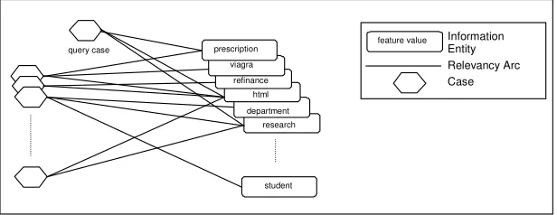
A CRN is a memory structure which allows an efficient yet flexible retrieval of cases. They borrow ideas from neural networks and associative memory models. They are made up of the following components:

• Case nodes represent stored cases.

• Information Entity Nodes (IEs) represent feature-value pairs within cases

• Relevance Arcs link case nodes with the IEs that represent them. They have

weights that capture the importance of the IE.

• Similarity Arcs connect IEs that refer to the same features, and have

weights relative to the similarity between connected IEs.

The idea behind the CRN architecture is that a target case is activated by connecting it to the net via a set of relevance arcs and this activation is then spread across the net. Each of the other case nodes accumulates an activation score appropriate to its similarity to the target case. The case nodes with the highest activation are the most similar cases to the target case.

We implemented a CRN for case retrieval that was configurable for different k -nearest neighbour classifiers. As the features in our case representation are binary (implemented as boolean values), IEs are only included for features with a true value and similarity arcs are not needed. The relevancy arcs are all weighted with a weight of 1.

Fig. 1 depicts an example of our CRN for spam filtering. Our implementation of the CRN is similar in some respects to a Concept Network Graph (CNG) [17] with thresholds set so that the activations are not spread beyond the first level of nodes.

refinance viagra prescription

department html

student research

feature value Information Entity Relevancy Arc Case query case

Fig. 1. Case Retrieval Net

3.5 Case Base Management

Case base editing techniques involve reducing a case base or training set to a smaller number of cases while endeavouring to maintain or even improve the generalisation accuracy. There is significant research in this area [18-20]. The case base editing technique that we used is Competence Based Editing [1] that uses the competence properties of the cases in the case base to identify noisy and redundant cases to remove.

The Competence Based Editing technique initially builds a competence model of the case base identifying for each case its usefulness (represented by the cases that it contributes to classifying correctly) and also the damage that it causes (represented by the cases that it causes to be misclassified). These properties of each case are used in a two step process to identify the cases to be removed. The first stage is the competence enhancement or noise reduction stage which removes mislabelled or exceptional cases. The second stage is the competence preservation or redundancy reduction stage. Redundant cases are those that are in the centre of a cluster of cases of the same classification and are not needed for classification.

The advantage of our CBE technique applied to the spam domain is that it results in a conservative pruning of the case base which we found resulted in larger case bases but better generalisation accuracy [1].

4

Static Evaluation

Two types of evaluation of ECUE were performed. Firstly, evaluations on 4 static datasets of 1000 emails each were performed to determine which feature representation was appropriate for the cases in the case base and to evaluate how a case-based classifier would perform compared to a Naïve Bayes classifier. These evaluations are discussed in this section. The second type of evaluation, the performance of the case-based system, ECUE, in a dynamic situation is discussed in Section 5.

It is worth noting that rudimentary feature extraction techniques, described in Section 3, were used for all evaluations. To achieve a high performance comparable with existing commercial spam filtering systems, such as Spamassassin, “commercial grade” feature extraction techniques need to be implemented.

4.1 Experimental Setup

The objectives of the static evaluations were two-fold, to determine the most appropriate case representation and to compare a case-based classifier with a Naïve Bayes classifier. Four datasets were used. The datasets were derived from two corpora of spam and legitimate email collected by two individuals over a period of approximately eighteen months up to and including December 2003 for Dataset 1 and up to and including January 2004 for Dataset 2. The legitimate emails in each corpus include a variety of personal, business and mailing list emails.

2003 and November 2003. Given the evolving nature of spam it was felt that these datasets gave a representative collection of spam.

4.2 Evaluation Metrics

Since FPs are much more serious that FNs, accuracy (or error) as a measure of performance does not present the full picture. Two filters with similar accuracy may have very different FP and FN rates.

In previous work on spam filtering a variety of measures have been used to report performance. The most common performance metrics are precision and recall [9]. Sakkis et al. [3] introduce a weighted accuracy measure which incorporates a measure of how much more costly an FP is than an FN. Although these measures are useful for comparison purposes, the actual FP and FN rate are not visible so the true effectiveness of the classifier is not evident. For these reasons, where appropriate, we will use the rate of FPs, the rate of FNs, and the average within class error rate,

AvgError = (FPRate+FNRate)/2 as our evaluation metrics.

4.3 Evaluation of Feature Representation

The objective of this evaluation was to determine whether a binary or numeric feature representation resulted in better generalisation accuracy. For each dataset we used 50 fold cross-validation, dividing the dataset into 50 stratified divisions or folds. Each fold in turn is considered as a test set with the remaining 49 folds acting as the training set.

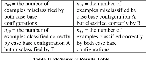
For each test fold and training set combination we built two case bases, the first using a binary feature representation for the cases and the second using numeric features. Section 3.2 discusses how these representations were achieved. Each case base representation was then edited using CBE (see Section 3.5). We then calculated the performance measures of the test set against each of the four case base configurations; binary and numeric feature representation, edited and not edited. Confidence levels were calculated using McNemar’s test [21] between each combination of two case base configurations to determine whether significant differences existed. For each test example the result is recorded and, in order to compare case base configuration A with B, a table such as Table 1 is constructed.

n00 = the number of examples misclassified by both case base

configurations

n01 = the number of examples misclassified by case base configuration A but classified correctly by B

n10 = the number of

examples classified correctly by case base configuration A but misclassified by B

n11 = the number of

examples classified correctly by both case base

configurations Table 1: McNemar’s Results Table

statistic in Equation 4 to be calculated. This statistic is distributed (approximately) as

2

χ with 1 degree of freedom.

(

)

The advantage that McNemar’s test has over the cross-validated paired t-test is a lower Type I error (the probability of incorrectly detecting a difference when no difference exists) but it also has good power (the ability to detect a difference where one exists) [21].

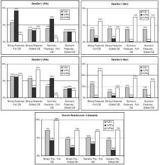
The results of our evaluations for each dataset and the average over all datasets are presented in Fig 2. It is worth noting that in the overall results, since we are calculating confidence levels using 4000 test examples, significance can be observed where the effect is quite marginal.

DataSet 1 (Feb)

5.7% 3.7% 4.0% 3.0% 9.2% 3.4% 6.8% 3.0% 2.2% 4.0% 1.2% 3.0% 0% 5% 10% Binary Features

- Full CB Binary Features- Edited CB Features - FullNum eric CB Num eric Features -Edited CB %Err %FPs %FNs

DataSet 1 (Nov)

3.7% 4.0% 3.8% 3.8%

1.2% 1.0% 0.2% 0.2% 6.2% 4.0% 7.4% 7.4% 0% 5% 10% Binary Features - Full CB

Binary Features - Edited CB

Num eric Features - Full

CB Num eric Features -Edited CB %Err %FPs %FNs

DataSet 2 (Feb)

6.4% 5.7% 3.3% 2.5% 6.2% 3.0% 5.8% 2.8% 6.6% 8.4% 0.8% 2.2% 0% 5% 10% Binary Features - Full CB

Binary Features - Edited CB

Num eric Features - Full

CB Num eric Features -Edited CB %Err %FPs %FNs

DataSet 2 (Nov)

12.3%

5.2%

9.0%

7.6%

0.4% 1.8% 0.6% 0.4%

24.2% 8.6% 17.4% 14.8% 0% 10% 20% 30% Binary Features - Full CB

Binary Features - Edited CB

Num eric Features - Full

CB Numeric Features -Edited CB %Err %FPs %FNs

Overall Results (over 4 datasets)

7.0%

4.7% 5.0% 4.4%

4.3%

2.3%

3.4%

1.6% 9.8%

7.0% _6.7% 7.2%

0% 5% 10%

Binary Ftrs - Full CB

Binary Ftrs -Edited CB

Numeric Ftrs - Full CB

Numeric Ftrs -Edited CB %Err %FPs %FNs

The results can be summarised as follows:

(i) Case base editing improves performance for both case representations although the performance for numeric features is not as significant (It only measures as significant at 95% confidence level for the overall result across all datasets whereas 2 of the 4 datasets demonstrate significant improvement for binary features at 99% level or higher with an overall significance level of 99.9%).

(ii) Case base editing also improves the performance on FPs with the binary feature representation showing higher levels of significance.

(iii) Using numeric features on a full (non-edited) case base has significantly better performance (at 99% or higher) than binary features in 3 of the 4 datasets. However, the FP performance is not significantly different except in Dataset 1 (Feb) (at the 95% level).

(iv) The performance of an edited case base with binary features is not consistently significantly better than a full or edited case base with numeric features.

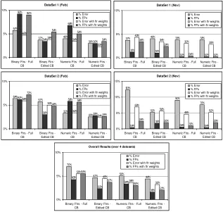
We then evaluated whether feature weighting improved performance or not. Each feature was weighted with a weight equal to the IG value of the feature identified during the feature selection process as suggested by Sakkis et al. [3]. We evaluated each case base configuration with and without feature weighting. The results are shown in Fig 3.

The results can be summarised as follows:

(i) Using feature weights has a negative effect on FP performance, with 5 of the 12 comparisons showing a significant difference (at 95% or higher) indicating that the rate of FPs is better without feature weighting. The remaining comparisons have no significant difference.

(ii) Using feature weights significantly improves the accuracy only in Dataset 2 (Nov) where 3 of the 4 comparisons show a lower error rate, with feature weighting, significant at 99% or higher. The remaining datasets do not demonstrate any significant improvement using feature weighting. Looking at the overall results for feature weighting, the best performance appears to be using numeric features on an edited case base. There is a significant difference in accuracy (at the 99.9% level) using feature weighting, but no significant difference in FP rate. A close second is using binary features on an edited case base with no feature weighting. The accuracy is not as good (a difference of 1.5%) significant at the 99.9% level but the difference in FP rate is not significant. Therefore in terms of classification accuracy, numeric features on an edited case base using feature weights wins.

rate is not affected. We expect that including domain specific feature extraction methods will improve the accuracy.

DataSet 1 (Feb)

5.7% 3.7% 4.0% 3.0% 9.2% 3.4% 6.8% 3.0% 4.7% 3.8% _3.4% 2.3% 9.0% 5.4% _5.0% 3.4% 0% 5% 10%

Binary Ftrs - Full

CB Binary Ftrs -Edited CB Numeric Ftrs - FullCB Numeric Ftrs -Edited CB % Error % FPs % Error with ftr weights % FPs with ftr weights

DataSet 1 (Nov)

3.7% 4.0% 3.8% 3.8%

1.2% 1.0% 0.2% 0.2% 4.3% 3.4% _3.0% 2.8% 3.4% 2.4% 0.4% 0.2% 0% 5% 10%

Binary Ftrs - Full

CB Binary Ftrs -Edited CB Numeric Ftrs - FullCB Numeric Ftrs -Edited CB % Error % FPs % Error with ftr weights % FPs with ftr weights

DataSet 2 (Feb)

6.4% 5.7% 3.3% 2.5% 6.2% 3.0% 5.8% 2.8% 5.9% 5.0% 3.4% 2.4% 7.2% 4.8% 5.6% 2.6% 0% 5% 10%

Binary Ftrs - Full

CB Binary Ftrs -Edited CB Numeric Ftrs - FullCB Numeric Ftrs -Edited CB % Error % FPs % Error with ftr weights % FPs with ftr weights

DataSet 2 (Nov)

12.3% 5.2% 9.0% 7.6% 0.4% 1.8% 0.6% 0.4% 6.9% 5.6% 4.6% 5.2% 2.4% _2.0% 1.0% 2.0% 0% 5% 10% 15%

Binary Ftrs - Full

CB Binary Ftrs -Edited CB Numeric Ftrs - FullCB Numeric Ftrs -Edited CB % Error % FPs % Error with ftr weights % FPs with ftr weights

Overall Results (over 4 datasets)

7.0%

4.7% 5.0% _4.4%

4.3% 2.3% 3.4% 1.6% 5.5% 4.5% 3.6% 3.2% 5.5% 3.7% 3.0% 2.1% 0% 5% 10%

Binary Ftrs - Full

CB Binary Ftrs -Edited CB Numeric Ftrs - FullCB Numeric Ftrs -Edited CB % Error

% FPs % Error with ftr weights % FPs with ftr weights

Fig 3: Results of Feature Weighting Evaluation

4.4 CBR vs NB

A key objective was to evaluate the generalisation accuracy of ECUE using a k-NN classifier with different values of k. A number of k-NN classifiers were evaluated. Once the k-NN classifier returns the cases that are determined to be closest to the query case, a voting algorithm is implemented to determine the classification of the query case. For this evaluation we used a distance weighted voting algorithm. The vote returned for classification ci for query case xq, over the k nearest neighbours

x1,…,xk using distance weighted voting is given in Equation 5 where 1(a,b)=1 if

b

a= , 1(a,b)=0if a≠b, wj is given in Equation 6 and cj is the classification of neighbour xj. The classification with the highest vote is deemed to be the classification of the query case.

) , ( 1 ) ( 1 = = k j i j j

i w c c

c

2

1

) ( )

( −

=

=

n

m

j m q m

j a x a x

w (6)

The votes for spam and non spam are normalised and the spam normalised vote is compared with a set threshold. If the spam vote is greater than the threshold the query case is considered to be spam. By varying the threshold from 0 to 1 and plotting the resulting rate of False Positive (FP) classifications (legitimate emails classified incorrectly as spam), against 1 minus the rate of False Negative (FN) classifications (spam emails classified incorrectly as legitimate), an ROC curve can be plotted [22].

In order to compare ECUE with the current spam filtering technique of choice, a NB classifier was implemented using the algorithm described in Section 2.1. Normalising the probabilities returned by the NB algorithm and varying the threshold for a spam classification as described above allowed an ROC curve to be plotted for the NB classifier. The larger the area under the curve for an ROC curve, the better the classifier. The results of the best k-NN classifier, for an edited and non edited case base and the NB classifier are presented in Fig. 4. To show the detail of the curve more clearly, only the top left hand corner of the graphs are presented.

The results presented above do not show that one classifier outperforms in all cases. NB seems to perform best in the February datasets while the k-NN classifier on an edited case base performs best in the November datasets.

DataSet Feb-1 - ROC curves

0.6 0.8 1

0 0.2 0.4

FPs

1-F

N

s _{k=5 (edited CB)}

k=5 (full CB) Naive Bayes

DataSet Nov-1 - ROC curves

0.6 0.8 1

0 0.2 0.4

FPs

1-F

N

s k=5 (edited CB)

k=5 (full CB) Naive Bayes

DataSet Feb-2 - ROC curves

0.6 0.8 1

0 0.2 0.4

FPs

1-F

N

s k=3 (full CB)

k=3 (edited CB) Naive Bayes

DataSet Nov-2 - ROC curves

0.6 0.8 1

0 0.2 0.4

FPs

1-F

N

s k=3 (full CB)

k=3 (edited CB) Naive Bayes

Fig. 4. Results of comparing different classifiers

5

Dynamic Evaluation

training data with examples of spam and legitimate email that were incorrectly classified.

5.1 Experimental Setup

Two datasets were used. The datasets were derived from the same two corpora of email as described above. A case base of 1000 cases, 500 spam emails and 500 legitimate emails were set up in each case. This training data included the last 500 spam and non spam emails received up to and including February 2003 in the case of Dataset 1 and up to and including January 2003 in the case of Dataset 2. This left the remainder of the data for testing. Table 2 shows the number of spam and legitimate emails received each month for both datasets.

A case base was set up for each training dataset using binary word and letter features. The classifier selected was k-nearest neighbour with k = 3. Due to the fact that an FP is much more serious than an FN, the classifier used unanimous voting to determine whether the target case was spam or not. All neighbours returned had to have a classification of spam in order for the target case to be classified as spam. This corresponds to the leftmost point on the ROC curve in Fig. 4. This strongly biases the classifier away from false positives.

Each case base was edited using the k-NN classifier with k = 3 and the CBE editing technique. Our previous experiments with case editing using CBE and a unanimous voting classifier indicated that generalisation accuracy increased using an edited case base [1]. Each email in the testing datasets, documented in Table 2, was presented for classification in date order to closely simulate what would happen in a real-time situation.

Table 2: Profile of the testing data Feb

‘03 Mar Apr May Jun Jul Aug Sep Oct Nov Dec Jan ‘04 Tot

Data

Set 1 spam 629 314 216 925 917 1065 1225 1205 1830 576 8902 non

spam 93 228 102 89 50 71 145 103 85 105 1076

Data

Set 2 spam 142 391 405 459 406 476 582 1849 1746 1300 954 746 9456 non

spam 151 56 144 234 128 19 30 182 123 113 99 130 1409

5.2 Evaluation Methods

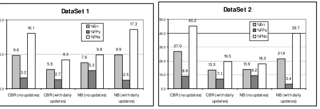
DataSet 1

9.6

5.5

7.6

9.9

3.2 2.7

5.3

2.5 16.1

8.3 9.8

17.3

0.0 10.0 20.0

CBR (no updat es) CBR (wit h daily updat es)

NB (no updat es) NB (wit h daily updat es) %Err

%FPs %FNs

DataSet 2

27.0

13.3 13.6

21.6

8.8 _7.1 9.2

3.4 45.2

19.5 _18.0

39.7

0.0 10.0 20.0 30.0 40.0 50.0

CBR (no updat es) CBR (wit h daily updat es)

NB (no updat es) NB (wit h daily updat es) %Err %FPs %FNs

Fig. 5. Results of evaluations over a period of time

The same experiments were performed using the NB classifier on unedited training data. The training data could not be edited for the NB classifier as the editing technique is a competence-based editing technique which uses a k-NN classifier to determine the competence of each case in the case base and analyses the competence properties of the cases to determine which cases should be removed. Due to the significance of FPs, the NB classifier was configured to be biased away from false positives by setting the threshold equal to 1.0. Fig. 5 includes the results of using NB.

5.3 Results

Although NB has a lower overall error rate over the datasets with no updating, the CBR system performs better in both datasets when dynamically updating the data to learn from incorrectly classified emails. It can be seen that daily updating of the training data with misclassified emails improves performance of the CBR system but has an overall detrimental effect on the NB classifier. NB with daily updates does improve the FP rate more than ECUE but the degradation of the FN rate has an overall negative effect on performance.

CBR only needs individual marker cases to construct its model whereas NB requires a full concept description. This may affect the performance of the NB classifier however the need to train the NB classifier on a full set of data presents its own set of data management problems.

It is worth noting that updating a system using NB with any new training data requires a separate learning process to recalculate the probabilities for all features. Updating a CBR system, such as ECUE, with new training data simply requires new cases to be added to the case base.

6

Future Work

The focus of the research presented in this paper is on the case base classifier’s ability to dynamically update the training data as new examples of spam and non spam are encountered. However, we envisage a hierarchy of learning within this domain where this continuous updating with misclassified emails is only the first level within three levels of learning.

training data. This level of retraining may need to be performed infrequently, e.g. every month or every other month. The highest level of learning, performed even more infrequently than feature selection, is to allow new feature extraction techniques to be added to the system. For instance, when domain specific features are used in the system, new feature extraction techniques will allow new features to be included. The benefit of using a CRN for implementing the second and third levels of learning is that it can easily handle cases with new features. The fact that these features may be missing in old cases is not a problem.

Future work on our CRN will also incorporate CNG-type activation spreading to allow cases that do not include the actual selected features to influence the classification process.

7

Conclusions

The initial stage of this research focused on identifying the most appropriate case base configuration for a case-based classifier for spam filtering. Evaluations indicated that the best accuracy was provided by a numeric feature representation using feature weighting. However, this benefit is marginal (1.5% in accuracy and not significant on the all important FP figures) and using numeric features has a significant impact on the speed of the system, particularly at the case editing stage. For this reason we are inclined to stay with the binary representation and seek to achieve accuracy improvements from improved feature extraction techniques. An alternative is to seek to speed up the editing of a case base that incorporates numeric features using caching of similarity scores for case pairs.

Using CBR for spam filtering is certainly no worse than using NB. As techniques which utilise a probabilistic classifier to detect spam e-mail are already patented [24], it is necessary to find other techniques which offer at least comparable results. In fact, our research suggests that CBR demonstrates better performance for learning over time than NB. CBR as a lazy learner offers significant advantages; it provides capabilities to learn seamlessly without the need for a separate learning process and facilitates extending the learning process over different levels of learning.

References

1.Delany SJ., Cunningham P.: An Analysis of Case-Based Editing in a Spam Filtering System, to be presented at 7th _{European Conference in Case-Based Reasoning (2004)}

2.Androutsopoulos, I., Koutsias, J., Paliouras, G., Karkaletsis, V., Sakkis, G., Spyropoulos, C., Stamatopoulos, P.: Learning to Filter Spam E-mail: A Comparison of a Naive Bayesian and a Memory-Based Approach. 4th _{PKDD Workshop on Machine Learning and}

Textual Information Access. (2000)

3.Sakkis G., Androutsopoulos I., Paliouras G., Karkaletsis V., Spyropoulos C.D., Stamatopoulos P.: A Memory-Based Approach to Anti-Spam Filtering for Mailing Lists. Information Retrieval, 6 (1), Kluwer Academic Publishers (2000) 49-73

5.Sahami M., Dumais S., Heckerman D., Horvitz E.: A Bayesian Approach to Filtering Junk Email. AAAI-98 Workshop on Learning for Text Categorization. AAAI Technical Report WS-98-05 (1998) 55-62

6.Androutsopoulos I., Koutsias J., Konstantinos V., Chandrinos V., Paliouras G., Spyropoulos C.: An evaluation of Naive Bayesian Anti-Spam Filtering. Proc. of the Workshop on Machine Learning in the New Information Age. G. Potamias, V. Moustakis and M. van Someren (eds.), 11th European Conference on Machine Learning, Barcelona, Spain (2000) 9-17

7.Androutsopoulos I., Paliouras G., Michelakis E.: Learning to Filter Unsolicited Commercial E-Mail, Tech rpt 2004/2, NCSR "Demokritos", (2004) http://www.iit.demokritos.gr/skel/i-config/publications/

8.Drucker HD., Wu D., Vapnik V.: Support Vector Machines for Spam Categorization. IEEE Transactions On Neural Networks, 10(5) (1999) 1048–1054

9.Gee K.R.: Using Latent Semantic Indexing to Filter Spam. Proceedings of the 2003 ACM Symposium on Applied Computing (SAC) Melbourne, FL, USA. ACM (2003) 460-464 10.Cunningham P., Nowlan N., Delany S.J., Haahr M.: A Case-Based Approach to Spam

Filtering that Can Track Concept Drift, The ICCBR'03 Workshop on Long-Lived CBR Systems, Trondheim, Norway,. (2003)

11.Lewis D., Ringuette M.: Comparison of Two Learning Algorithms for Text Categorization. SDAIR (1994) 81-93

12.Niblett: Constructing Decision Trees in Noisy Domains. Proceedings of the Second European Working Session on Learning. Bled Yugoslavia Sigma (1987) 67-78

13.Kohavi R., Becker B., Sommerfield D.: Improving Simple Bayes. ECML-97 Proceedings of the Ninth European Conference on Machine Learning (1997)

14.Quinlan J. R.: C4.5 Programs for Machine Learning. Morgan Kaufmann Publishers, San Mateo, CA. (1997)

15.Yang Y., Pedersen J.O.: A Comparative Study on Feature Selection in Text Categorization. Proceedings of ICML-97 14th Int Conf on Machine Learning. Nashville, US,. (1997) 412–420.

16.Lenz M., Auriol E., Manago M.: Diagnosis and Decision Support. M. Bartsch-Sporl, H. D. B., and Wess, S., eds., Case-Based Reasoning Technology: From Foundations to Applications, LNCS Vol 1400. Springer-Verlag (1998)

17.Ceglowski M., Coburn A., Cuadrado J.: Semantic Search of Unstructured Data using Contextual Network Graphs. http://www.nitle.org/semantic_search.php

18.McKenna E., Smyth B.: Competence-Guided Editing Methods for Lazy Learning. Proceedings of the 14th European Conference on Artificial Intelligence, Berlin (2000) 19.Wilson D.R., Martinez T.R.: Instance Pruning Techniques. Proceedings of the 14th _Int.

Conference on Machine Learning, Fisher D. (ed.). Morgan Kaufmann, San Francisco, C.A. (1997) 404-411

20.Brighton H., Mellish C.: Advances in Instance Selection for Instance-Based Learning Algorithms. Data Mining and Knowledge Discovery, Vol 6. Kluwer Academic Publishers (2002) 153-172

21.Dietterich T.G. Approximate Statistical Tests for Comparing Supervised Classification Learning Algorithms. Neural Computation 10 (1998) 1895-1923

22.Bradley A.P.: The Use of the Area under the ROC Curve in the Evaluation of Machine Learning Algorithms. Pattern Recognition, Vol 30. (1997) 1145-1150.

23.Baeze-Yates R., Ribeiro-Neto B.: Modern Information Retrieval. Addison-Wesley, ACM Press New York (1999)