Dynamical determinants and their applications

(1)

University of Warwick institutional repository: http://go.warwick.ac.uk/wrap

A Thesis Submitted for the Degree of PhD at the University of Warwick

http://go.warwick.ac.uk/wrap/54674

This thesis is made available online and is protected by original copyright. Please scroll down to view the document itself.

(2)

Dynamical Determinants and their Applications

by

Philip Felton

Thesis

Submitted to The University of Warwick

for the degree of

Doctor of Philosophy

Mathematics Institute

(3)

Chapter 1 Introduction

The general theme of this work is to examine a variety of settings in which transfer operators can be defined and be shown to be trace class, so that we may then define the associated dynamical zeta function, enabling us to finally say something useful about appropriate characteristics in that setting. Previous examples include the following:

• Jenkinson and Pollicott (22; 23) approximate the Hausdorff dimension of re-pellers of analytic expanding maps, using Bowen’s pressure formulaP(₋slog_|T0_|) = 0 where T is the map restricted to the repeller, and s is then the Hausdorff dimension of the repeller. This applies, for example, to hyperbolic Julia sets, and limit sets of convex cocompact Fuchsian groups. It offers an alternative to an earlier method of McMullen who used the transfer operator more directly to estimate solutions of P(₋slog_|T0_|) = 0, without using a zeta function.

• In (24), the same authors exhibit a super-exponentially converging numerical integration technique for analytic functions on the closed unit intervalI. This relies on knowing the value of the function on a uniform set of points (the fixed points of Tn _for _T₍_x_{) = 2}_x_{(mod 1)). This can be generalised to functions on}

In_{. This method is efficient amongst algorithms which use values at evenly}

(9)

1. Introduction 2

distributed points, although other algorithms can be more efficient by choosing points to sample as part of the algorithm.

• Their paper (21) estimates the absolutely continuous invariant measure den-sity function for a piecewise analytic expanding map T of the interval. The density function for the absolutely continuous invariant measure here is an analytic function, and it can be expanded as a Fourier series. They estimate the individual Fourier coefficients using periodic points of the transformation

T.

• Pollicott and Rocha (45) calculate the determinant of the Laplacian on a manifold of constant negative curvature. The Laplacian is a second order self-adjoint linear operator which has countably many eigenvalues. The de-terminant of the Laplacian is a spectral invariant, formally defined via the meromorphic extension of a suitable complex function. The determinant is an important geometric characteristic. There are now other, more accurate, approximations of this quantity, see (60).

Transfer operators perform a kind of averaging on a function, where the points to sample are pre-images of an underlying transformation. They arose from statis-tical physics, and were first studied by Ruelle (47). His work established them as interesting objects in their own right. They were first applied to symbolic codings of dynamical systems, i.e. subshifts of finite type, on Banach spaces of Lipschitz continuous functions. This work was popularised by Bowen’s book (7), which unified the ideas of Ruelle with Sinai’s paper on Gibbs measures (56).

(10)

1. Introduction 3

transfer operator has a spectral gap. The key ingredient in the proof is what Ruelle called the ‘basic inequality’, and is now commonly referred to as the Lasota-Yorke inequality, however in different settings, it is much older (W. Doeblin and R. Fortet in 1937 showed quasi-compactness for a particular family of operators. In 1948 T. Ionescu and G. Marinescu generalised this result to obtain it for a larger family).

The Lasota-Yorke inequality is also used to show more abstract results, not just about transfer operators on subshifts of finite type, for example Nussbaum’s formula for the essential spectral radius (36), and Hennion’s theorem that in particular gives conditions for an operator to be quasi-compact. Other examples of its uses include the work of Hofbauer and Keller (18) who applied the inequality in the context of expanding interval maps with bounded variation functions, Pollicott (41) who used the inequality to study subshifts of finite type and Gibbs measures, and Liverani

et al who considered operators for invertible transformations. The book of Hen-nion and Herv´e (17) has a detailed description of the general method. Liverani’s work provided a new perspective, where expanding maps were replaced by diffeo-morphisms, by means of special distributional Banach spaces. However, there is not yet a theory of determinants for this setting.

An important application of transfer operators is to find absolutely continuous invariant measures for certain types of transformations. Such a measure exists, for example, when T is C2 and expanding, in this case originally due to the work of Lasota and Yorke (28) which generalised earlier results for more specific maps. In these circumstances we can define a transfer operator _L which has a positive fixed point φ0, and whose dual preserves the Lebesgue measure. It then follows that

R

f_◦T _·φ0dm =

R

f φ0dm wherem is the Lebesgue measure, i.e. the measure φ0dm

(11)

1. Introduction 4

An advantage of studying transfer operators is that they often preserve a space of higher regularity, depending on the underlying transformation T. Assume T is expanding, and the weight is 1/_|T0_|. Under these assumption, for example, if T is

Ck_, _k _∈

N, then L(Ck−1) ⊂ Ck−1. If T is C1+α then L preserves Cα (α-H¨older continuous functions). The spectrum on the smaller spaces is often smaller, and eigenvalues in the smaller space are also in the larger one.

It is possible to define transfer operators in a variety of settings, but we are interested in the case when they work on Banach spaces of holomorphic functions, so that we can use the work of Grothendieck and also obtain convenient trace formulae. At the beginning of the 20th century, Fredholm studied integral equations, where the general problem is to find a function f, given a function g and a kernel K (in some spaces) satisfying:

g(t) =

Z

K(s, t)f(s)ds.

Fredholm showed that the integral operator Lf(t) = R K(s, t)f(s)ds is trace-class, and defined

det(I ₋zL) = exp ₋

∞ X

n=1

zn

n trL

n

!

,

and this definition is natural because for finite matrices, it is an identity. For suitable conditions on the kernel, this gives us an entire function whose zeros are related to eigenvalues of the operator, and a product formula holds,

det(I₋zL) =

∞ Y

n=1

(1₋zλn),

where (λn)n∈Nis the eigenvalue sequence, in decreasing order of magnitude, repeated

(12)

1. Introduction 5

rate of convergence. It became a general problem to find conditions on operators which ensures that their eigenvalue sequence is well behaved, e.g. belongs to `p _for 0< p <_∞.

Grothendieck (13) defined the class of nuclear operators, and proved that any nuclear operator has a square-summable eigenvalue sequence. This was notable in that it applies in the more general setting of Banach spaces rather than Hilbert spaces. A linear operatorL : _B1 → B2 between Banach spaces B1 andB2 is nuclear

of order p_≥0 if there exists sequences of elements (un)n∈N inB2 of unit length, and

linear functionals (`n)n∈_N in B₁? such that Lx = P∞_n₌₁`n(x)un for all x ∈ B1, and

P∞

n=1k`nkq <∞for allq > p. Nuclear operators of order p <2/3 are trace class, so there is a bounded linear functional on nuclear operators _{B → B} which generalises the usual finite dimensional trace functional, and allows us to define the Fredholm determinant as above.

It is also interesting that a formal link between transfer operators and integral operators exists because a transfer operator can be thought of as an integral operator with a kernel given by K(x, y) =δ(T y₋x) where δ is the Dirac Delta function.

Ruelle (47) first studied transfer operators on spaces of holomorphic functions, since this setting could employ Grothendieck’s results. His paper establishes a gen-eral result about the transfer operator of the complexification of real analytic ex-panding maps on compact connected real analytic manifolds (that they are nuclear and have a particular equation for their traces), then applies this to express the Artin-Mazur and Smale zeta-functions as Fredholm determinants of specific trans-fer operators. In this paper, Ruelle claimed that det(I₋zL) for the transfer operator

Lhas a power series whose coefficients obey O(e−Cn2

(13)

1. Introduction 6

Zeta functions are meromorphic functions analogous to the famous Riemann zeta function in number theory - they are defined in terms of some objects we are interested in the cardinality or distribution of, and are useful for coding this information in the location of their zeros or poles. In dynamics, particular zeta functions can often be related to the Fredholm determinant of a particular transfer operator.

The use of zeta functions in dynamics arose from counting periodic orbits. For a map f : X _→ X, we wish to consider the asymptotic behaviour of the numbers #Fix(fn_{), where Fix(}_fn_{) =}_{_x_∈ _X _: _fn_x₌_x_}_{. The Artin-Mazur zeta function is} defined by

ζ(z) = exp

∞ X

n=1

zn

n #Fix(f

n₎

!

.

For example, for a subshift of finite type σ : ΣA→ΣA, given by the matrix A, the Bowen-Lanford result tells us that ζ(z) = (det(I ₋zA))−1, i.e. the zeta function is rational. This has a pole for z = 1/λ where λ is the largest eigenvalue of A, so we can read off the entropy from this zeta function, which tells us the asymptotic growth rate of the number of period orbits.

The Artin-Mazur zeta function can be generalised by introducing a weighting function. If f : M _→M is a map, and φ : M _→_Ca weight function, then we can define the Ruelle zeta function by

Z(φ) = exp



 ∞ X

n=1

1

n

X

x∈Fix(fn₎ n−1

Y

k=0

φ(fkx)





(14)

1. Introduction 7

surfaces of constant negative curvature,

Z(s) =Y γ

∞ Y

k=0

1₋e−(s+k)`(γ),

where the outer product is taken over all closed geodesics γ, and `(γ) is the length of γ. This is an entire function with trivial zeros at 0,₋1,₋2, . . . and zeros on (0,1) and Res = 1/2 which relate to the eigenvalues of the Laplacian operator on the surface. Smale generalised this zeta function to geodesic flows on surfaces of curvature ₋1, and proposed extending this to Axiom A flows.

In 1972 Bowen showed that the closed orbits of Axiom A flows are uniformly dis-tributed in the non-wandering set with respect to the measure of maximum entropy. Parry (37) gave an alternative proof using zeta functions. For Axiom A flows, a partial meromorphic extension of the zeta function follows from the work of Parry and Pollicott. For special Anosov flows, where the stable and unstable foliations are real analytic, the work of Ruelle related these to determinants.

The Grothendieck theory tells us that a trace functional exists for nuclear op-erators, however many uses of this theory require us to have an expression for the trace of a transfer operator. Ruelle (47) gave a formula for the trace, and this has since been generalised to operators on wider classes of function spaces by Mayer (31), and Bandtlow and Jenkinson (5), who also prove that eigenvalue sequence for certain transfer operators is in some sense universal; the eigenvalue sequence is de-termined by the weights and inverse branches, not the particular ‘favourable space’ of functions the transfer operator acts on.

An outline of the remainder of this work is as follows:

• Chapter 2 contains standard definitions and results required in the remainder of the work.

(15)

1. Introduction 8

of families of matrices. Motivated by the work of Pollicott on approximating the Lyapunov exponent for discrete families of matrices, we investigate many of the details, and attempt a generalisation for the case of continuous families. The main result in this chapter is a new expression for the Lyapunov exponent of the continuous case, albeit of limited numerical use as it stands. We also arrive at a slightly modified version of the approximation of Pollicott for the discrete case.

• Chapter 4 is concerned with extracting information from the spectrum of a particular transfer operator about eigenvalues and eigenfunctions of the Lapla-cian on a surface of constant negative curvature. We know that the zeros of the Selberg zeta function determine the spectrum of the Laplacian. Moreover the Selberg zeta function can be realized as the determinant of a suitable transfer operator, thus allowing the possibility of accurate computations of such values. Moreover we are interested in the more ambitious programme of estimating the associated eigenvectors.

• The subject of chapter 5 is Mahler measures, their numerical approximations, and a couple of applications. Mahler measures are a special type of integral as-sociated to polynomials, and in some cases we can apply the work of Jenkinson and Pollicott to enable numerical approximations. Their work uses dynamical determinants to derive a rapidly converging sequence converging to the value of an integral with Cω integrand. If the zeros of the polynomial are unfortu-nately located, we might hope to split the integral up at the location of this zero, and divide by a polynomial which removes the zero. This hopefully only changes the answer by an amount given by a standard integral.

(16)

1. Introduction 9

(17)

Chapter 2 Background Material

Throughout we denote an open ball in a metric space (X, d) centred at x _∈ X of radiusr >0 byBd(x, r), and when the metric used is unambiguous we writeB(x, r). Similarly for a normed vector space (X,_{k · k}) we use the notation Bk·k(x, r).

2.1 Functional Analysis

Let (_B,_{k · k}) denote a Banach space, and let L : _{B → B} be a linear operator. The quantity

kL_k= sup_{kLx_k : x_{∈ B},_kx_k= 1_}

is called theoperator normofL. If this is finite, we sayLis bounded, and we denote the set of all such bounded linear operators on _B as _L(_B).

The resolvent set res(L) of Lis the set of z _∈_Csuch that L₋zI has an inverse and (L₋zI)−1 _{∈ L}₍_B_{). The}_spectrum_of_L_{, sp(}_L_{), is the complement of the resolvent,}

sp(L) =_{z _∈_C : z /_∈res(L)_},

and is a compact subset of _C. The eigenvalues of L are defined as the points

λ _∈ sp(L) where L₋λI fails to be injective. The multiplicity of an eigenvalue is

(18)

2. Background Material 11

the dimension of the eigenspace _{v _{∈ B} : (L₋λI)v = 0_}, if this equals 1 we say the eigenvalue is simple. An eigenvalue λ is isolated if there exists δ >0 such that sp(L)_∩B(λ, δ) =_{λ_}. Any isolated point of the spectrum is an eigenvalue.

The spectral radiusR(L) ofL is

R(L) = sup_{|z_| : z _∈sp(L)_},

and the essential spectral radius Ress(L) is the smallest number Ress ≥ 0 such that

any eigenvalue λ_∈sp(L) with _|λ_|> Ressis an isolated eigenvalue of finite

multiplic-ity. If Ress(L)< R(L), the operator is called quasicompact.

An operator L _{∈ L}(_B) is compact if the image _{Lxn : n ∈ N} of any bounded sequence (xn)n∈N inB contains a Cauchy sequence. An operator L is finite rank if the image L(_B) is finite-dimensional. Finite rank operators are compact.

The dual of _B is the set _B? _{of bounded linear functionals} _φ _: _{B →}

C and is a Banach space with the operator norm. The dual L? _: _B? _{→ B}? _{of an operator}

L_{∈ L}(_B) is defined by

(L?φ)(x) = φ(Lx),

for all φ _{∈ B}? and x_{∈ B}.

We now define what it means for a map from an open subset of _C to a Banach space to be holomorphic, which we require for using the perturbation theorem.

Let U _⊂ _C be open and _B a complex Banach space. Consider f : U _{→ B}. Fix

x_∈U. If there exists a bounded complex-linear mappingL :_C_{→ B} such that

lim h→0

kf(x+h)₋f(x)₋L(h)_k

kh_k = 0

(19)

If f : U _{→ B} is locally bounded and the mapping

λ_7→φ(f(x+λ))

is holomorphic in the usual sense at λ = 0 for all x _∈ U, and bounded linear functionalsφ _{∈ B}?_{, we say} _f _is_{weakly holomorphic}_.

Fortunately these two definitions are equivalent (for a proof, see for example the lectures notes of Omri Sarig (52)), so a function that satisfies either is called holomorphic. Holomorphic functions are closed under addition, multiplication by scalar, and composition. We can also extend this definition to say that a map

f : _B1 → B2 between two Banach spaces is holomorphic if f ◦g is holomorphic

whenever g :_C_{→ B}1 is holomorphic.

If we restrict ourselves to maps from _Cto a Banach space, we have the following result, which generalises some results in complex analysis of one variable. Proofs for these results can also be found in (52).

Proposition 2.1. Let U _⊂ _C be an open simply connected set, and _B a Banach space. Then

1. (Morera’s Theorem) f : U _{→ B} is holomorphic if and only if for every closed smooth curve γ in U, we have

I

γ

f(z)dz = 0.

2. (Cauchy’s Integral Formula) If f : U _{→ B} is holomorphic, any point ξ _∈ U, any closed smooth curve γ in U, and an integer n _≥0, we have

f(n)(ξ) = n! 2πi

I

γ

f(z) (z₋ξ)n+1dz.

(20)

is holomorphic if and only if there is a power series expansion

f(z) =f(z0) +

∞ X

n=1

an(z−z0)n, |z−z0|< r,

where an ∈ B for all n and the series converges uniformly in the norm of B

on compact subsets B(z0, r).

Let_{Lz}z∈U denote a family of operators inL(B), parameterised byz ∈U where

U _⊂_C is an open neighbourhood of zero. The family is called an analytic family if the map U _{→ L}(_B) given by z _7→ Lz is holomorphic. An important result about analytic families is the following, for a proof see Kat¯o’s book (26), or again (52).

Theorem 2.2. (Perturbation Theorem) Let _{Lz}z∈U be an analytic family of

oper-ators, such that L0 has an isolated simple eigenvalue λ. Then there exists an >0,

and a family _{λz}z∈B(0,) ⊂ C, such that λ0 = λ, the map z 7→ λz is holomorphic,

and λz is an isolated simple eigenvalue of Lz.

We also need to define a Banach space of holomorphic functions, which provides us with a space on which to define trace-class transfer operators. Let D be a open, bounded and connected set in _Cn.

Definition 2.3. We denote by Hol(D) the Fr´echet space of holomorphic functions

D _→ _C, and by C(D) the Banach space of continuous functions D _→ _C with the supremum norm. We finally define the set

F(D) =_{f _∈C(D) : f_|D ∈Hol(D)},

and the norm _{k · k}F(D) by

kf_kF(D) = sup

z∈D |f(z)_|

(21)

Here, ‘holomorphic’ means holomorphic in the single variable case in each vari-able separately. Many of results in single varivari-able complex analysis generalise, in par-ticular Montel’s theorem (see the book of Krantz (27)), which makes (F(D),_k·kF(D))

into a Banach space. We will make use of Morera’s theorem on each variable sepa-rately to show membership of this space.

Another common space is L2(D)_∩Hol(D) which we denote L2_ω(D). We have that F(D)_⊂L2

ω(D) but they do not co-incide because for example whenD =D= {z _∈ _C : _|z_| < 1_} the function f(z) = (z ₋1)−1/2 _{is not bounded in}

D so is not a member of F(_D). However, by using the substitutionz = 1 +reiθ_{, we have}

Z

D

|f(z)_|2dxdy_≤

Z 2

0

Z π

−π

(1/r)rdrdθ = 4π < _∞,

hence f _∈L2

ω(D).

2.2 Nuclear Operators

The theory in this section is mostly due to Grothendieck, see (13), and generalises the situation of integral operators considered by Fredholm. A relevant survey is in Ruelle’s book (49), and many of the details may be found in the books of Ryan (51), Pietsche (39), and Schaefer (53).

As part of a very brief account of nuclear operators, we define tensor products of Banach spaces. One way to construct the tensor product of two Banach spaces X

andY is as follows. The tensor productx_⊗yof elementsx_∈Xandy_∈Y is a linear functional onB(X_×Y), the set of bilinear forms. It is given by (x_⊗y)(A) =A(x, y). The tensor product X _⊗ Y is then the the subspace of B(X _×Y)? _{spanned by} the elements x _⊗y. An element u _∈ X _⊗Y is given by u = Pn

(22)

representation is not unique. We define the projective norm π onX_⊗Y by

π(u) = inf

( _n

X

i=1

kxikkyik : u= n

X

i=1

xi⊗yi

)

,

and define the projective tensor product Banach space X_⊗ˆπY to be the completion ofX_⊗Y with respect to the projective norm. We have the following useful formula for the projective norm on X_⊗ˆ_πY:

π(u) = inf

( _∞

X

n=1

|λn| : u=

∞ X

n=1

λnxn⊗yn,kxnk= 1,kynk= 1

)

.

There is a canonical operator J : X?_⊗ˆπY → L(X, Y) of unit norm that associates

u=P∞

n=1φn⊗yn with the operator Lu : X →Y given by Lu(x) =

P∞

n=1φn(x)yn. We call the range of J the nuclear operators. They form a Banach space denoted by N(X, Y), with projective norm carried across. All nuclear operators are compact.

An important property of nuclear operators is that we can define their traces. Tensor product theory shows that there exists a functional Tr :_N(X)_→_C, which is continuous and coincides with the usual trace for finite dimensional spaces. It is defined by

Tru=

∞ X

n=1

φn(xn),

and this does not depend on the representation of u. Nuclear operators also form an ideal. If S : X _→ Y is a nuclear operator and T _{∈ L}(W, X) and R _{∈ L}(Y, Z), then RST is a nuclear operator.

We now turn to determinants of nuclear operators. For u_∈X?_⊗_ˆ

πX, defining

Det(1 +u) = 1 +

∞ X

n=1

X

i1<···<in

det(φil(xik)) n

l,k=1 (2.1)

makes sense because there is a similar formula in the finite case.

(23)

1. u_7→Det(1 +u) is an entire holomorphic function.

2. Det(1 +u)₆= 0 if and only if Lu is invertible in L(X).

3. If λ is an eigenvalue of multiplicity n for Lu then λ−1 is a zero of order n of

z _7→Det(1₋zu).

4. The identity

Det(1₋zu) = exp ₋

∞ X

n=1

zn

n Tru

n

!

(2.2)

holds where the power series converges for a neighbourhood of zero.

The rate in which the terms of u tend to zero gives further information, so we state the following definition.

Definition 2.5. An operator _L : X _→ X on a complex Banach space X is called nuclear of orderp_≥0 (alternatively,p-nuclear) if there exists sequences (λn)n∈N∈C,

(φn)n∈N∈ X

? _{and (}_x

n)n∈N ∈X with kφnk= 1 and kxnk= 1 for all n such that for allx_∈X:

Lx=

∞ X

n=1

λnφn(x)xn,

and P∞

n=1|λn|

q _< _∞ _{for all} _{q > p}_{. It is called strongly nuclear if it is nuclear of} order zero.

For each p_≥0, the p-nuclear operators form an ideal.

Proposition 2.6. Ifuisp-nuclear forp_≤2/3, then the eigenvalue sequence(λn)n∈_N

of Lu has

P∞

n=1|λn|p <∞ and

Tru=

∞ X

n=1

λn.

Furthermore we have the following usual connection between the determinant and

the trace:

Det(1₋zu) =

∞ Y

n=1

(24)

Example 2.7. Define the linear operator Ls : F(D) → F(D) by Lf(z) = f(z/s) for s > 1. Define the sequence (un)n∈_N0 of functions D → D by un(z) = z

n_{, which} is a basis for F(_D), and the dual basis (φn)n∈_N0 by φn(um) = 1 if n = m, and 0

otherwise. Clearly _kunkF(D)= supz∈_D|un(z)|= 1 andkφnk= 1 for alln ∈N0.

Fix an arbitrary f _∈ F(_D), and write it as f = P∞

n=0anun where (an)n∈N0 is a

sequence in _C. We can then write the operator as

Lsf(z) =

∞ X

n=0

anun(z/s) =

∞ X

n=0

an(1/s)nun(z) =

∞ X

n=0

(1/s)nφn(f)un(z).

Then Ls is of the form Lsf(z) = P

∞

n=0λnφn(f)un(z) where φn and un are

nor-malised, and λn = 1/sn. Now P

∞

n=0|λn|

p ₌ P∞

n=0(1/s

p₎n _< _∞ _{provided 1}_/sp _<_1, i.e. p > 0. This shows Ls is strongly nuclear.

Furthermore, since Ls(un) = 1/snun, we see that 1/sn is an eigenvalue for each

n _≥ 0. From this and the strong nuclearity we have that TrLs =

P∞

n=0s

−n ₌ 1/(1₋s−1_{). Since} _Ln

s =Lsn, we can see that TrLn_s = TrL_sn = 1/(1−s−n).

The standard ways of showing an operator is p-nuclear or strongly nuclear is using Cauchy’s theorem to obtain the linear functionals, or using the fact the space of nuclear operators is an ideal to factor an operator L into a composition RST

where R and T are any bounded linear operators, and S is an operator already known to be nuclear.

We also have a source of nuclear operators because some spaces are nuclear, that is spaces where any bounded linear operator from that space to any Banach space is nuclear. An example of a nuclear space is the Fr´echet space Hol(D) whereD _⊂_Cd

is a bounded, open, connected set.

We can give a power series expansion of the determinant using equation 2.2,

Det(1₋zu) = 1 +

∞ X

n=1

(25)

with the terms bn worked out as follows.

Det(1₋zu) = 1 +

∞ X

n=1

1

n! −

∞ X

m=1

zm mTru

m

!n

= 1 +

∞ X

n=1

(₋1)n

n!

∞ X

p=1

zp X

m₁,...,mn∈N

m1+···mn=p n

Y

i=1

Trumi

mi

= 1 +

∞ X

n=1

znbn,

where

bn =

X

n₁,...,nm∈_N n1+···nm=n

(₋1)m

m! m

Y

i=1

Truni

ni

. (2.3)

This is central to using this theory to construct quickly converging numerical ap-proximations to various quantities. This requires bounding the terms bn (and also requires a suitable expression for the trace, discussed later). Assume u is nuclear and can be written in the form u =P∞

n=1anφn⊗xn with kφnk =kxnk = 1 for all

n _∈_N, and the terms an∈C are controlled by

0<_|an|< Aαn

1/d

(2.4)

for constants A >0, 0 < α <1 and d_∈_N. First, equation 2.1 gives

bn =

X

i1<···<in

ai1ai2· · ·aindet(φil(xik)) n

l,k=1. (2.5)

By a result of Hadamard (14) we have that anyN_×N matrix with entries of modulus at most 1 has determinant with modulus bounded by NN/2_{, hence}

|bn| ≤nn/2An

X

i1<···<in

αi11/d+i21/d+···+in1/d_.

(26)

fα(z) = 1 +P

∞

n=1βn(α)z

n ₌Q∞

i=1(1 +α

i1/d

z), so that

|bn| ≤nn/2Anβn(α). (2.6) Fried (12) showed that βn(α) = O(δn

1+1/d

) where 0 < δ < 1, and Jenkinson and Pollicott in (23) reproduce Fried’s analysis. Fried used Cauchy’s estimate, then examined the number of zeroes in the ball _|z_| < r, to show that βn(α) ≤

r−n_exp(_a

αP(logr)) for allr >0 whereaα = (−logα)−d>0, andP(x) =

Pd+1

j=0

d!

j!x

j_. Define rn = exp((n/aα)1/d). Then βn(α) ≤ r−nnexp(aαP(logrn)) = O(n

1+1/d ) for any 1 > > αd/(d+1). Substituting this into equation 2.6 gives bn =O(δn

1+1/d ) for any < δ <1. This is summarised in the following proposition.

Proposition 2.8. If an operatorL is nuclear, and can be written in the form Lf =

P∞

n=1anφn(f)un, with kφnk= kunk= 1 and 0<|an|< Aα

n1/d

, A > 0, 0< α < 1, then the determinant det(1₋zL) = 1 +P∞

n=1bnzn has coefficients which decrease

super-exponentially fast. We have bn=O(δn

1+1/d

) for any αd/(d+1) _{< δ <}₁_.

Use of the Hadamard estimate doesn’t affect the rate of the convergence but it suggests that we lose information which might be used to tighten up the con-stant implied in the _O notation. For the case where d = 1, we can write _|bn| ≤

nn/2_An_αn2

αP(−nlogα) _where _P₍_x_{) = 1 +}_x₊_x2_/_2.

The bound on the (an)n∈_N sequence is usually established in practice using

Cauchy estimates. Alternatively, if a similar bound can be established on the eigen-values of the operator instead, we can obtain a similar result about the rate of convergence of the determinant.

Proposition 2.9. If a strongly nuclear operator _L has eigenvalues(λn)n∈N, and we

have a bound

0<_|λn|< Aαn

1/d

for all n, for some A > 0 and 0 < α < 1, then we have bn = O(δn

1+1/d

(27)

αd/(d+1) _{< δ <}₁_.

Proof. Since the operator is strongly nuclear we have

1 +X n=1

bnzn = det(1−zL) =

∞ Y

i=1

(1₋zλn) = 1 +

∞ X

n=1

(₋1)nzn X

i1<···<in

λi1· · ·λin,

so bn = (−1)nP_i₁_<···<inλi1· · ·λin. We can then bound

|bn| ≤An

X

i1<···<in

αi11/d+···in1/d_, and perform Fried’s analysis as before.

Example 2.10. Returning to example 2.7, we can write

det(1₋zLs) = exp −

∞ X

n=1

zn 1

n(1₋s−n₎

!

,

and also notice that the determinant of the matrix in equation 2.5 is now 1, hence the terms in the power series for the Fredholm determinant are in this case bounded by_|bn| ≤s−n

2

s−P(nlogs)_{. Here}_L

s is a composition operator, and the underlying map is a contraction, and we observe that the stronger the contraction ratio (the larger we make s) then the faster the rate of convergence of the determinant.

2.3 Transfer Operators

Transfer operators are usually of the following flavour. Consider a transformation

T :X _→X, on some space X, with T−1₍_x_{) countable or finite for each}_x_∈_X_{, and}

let g : X _→ _C be a weight function such that P

y∈T−1₍_{_x_}₎g(y) is convergent. Let

(28)

Lg :B → B is defined as

Lgf(x) =

X

y:T y=x

f(y)g(y).

The archetypal setting for transfer operators is subshifts of finite type. The reader is referred to the book of Parry and Pollicott (38) for more information and proofs. This setting arises for example as a result of looking at the coding of an expanding map on a Markov partition, or lattice spin systems in statistical physics. LetAdenote ak_×kmatrix with each entry either zero or one, which is furthermore aperiodic, i.e. some iterate An _{is strictly positive. Let} _S ₌_{₁_{, . . . , k}_}_and

Σ+_A =_{x_∈SN _: _A₍_x

n, xn+1) = 1 for all n}

with the Tychonov product topology. This topology is generated by cylinders, let

j _≥1 and x1, . . . , xn ∈S, then the cylinderZ(j;x1, x2, . . . , xn) is given by

Z(j;x1, x2, . . . , xn) ={y∈Σ+A : yj =x1, yj+1 =x2, . . . , yj+n=xn}.

Note that a cylinder might be empty. The topology is also metrizable. Given 0< θ <1 definedθ(x, y) = θN whereN = min{k|xk 6=yk}. The shiftσ : Σ+A →Σ

+

A

is then the transformation which deletes the first term in the sequence,σx=ywhere

yn=xn+1. For a function f : Σ+_A →Cand n ≥0 define

varnf = sup{|f(x)−f(y)| : xi =yi,0≤i≤n}

and

(29)

This is only a pseudo-norm, so define _kf_kθ =|f|∞+|f|θ. Let

F+

θ ={f : Σ

+

A →C : f continuous, kfkθ <∞},

the space of dθ-Lipschitz continuous functions.

Let g _{∈ F}_θ+. The Ruelle transfer operator _Lg : Fθ+ → F

+

θ , a bounded linear operator, is defined by

Lgf(x) =

X

σy=x

g(y)f(y).

The following important theorem, a generalisation of the classical Perron-Frobenius theorem, is due to Ruelle (48). In other settings for transfer operators, the hope is that similar results hold.

Theorem 2.11. (Ruelle-Perron-Frobenius) Let g _{∈ F}_θ+ be real valued and strictly positive.

1. There is a simple maximal positive eigenvalue β of _Lg with corresponding

strictly positive eigenfunction h_{∈ F}_θ+.

2. The remainder of the spectrum of _Lg is contained in a disc of radius strictly

less than β. Hence _Lg is quasicompact.

3. There is a unique σ-invariant probability measure µ such that µ(_Lg(v)) =

βµ(v) for all v _∈C(Σ+_A), the set of continuous functions on Σ+_A. 4. β−n_Ln

gv →h µ(v)/µ(h) uniformly for all v ∈C(Σ

+

A).

Ifgis real and strictly positive, the measureµfrom this theorem is an equilibrium state for logg, and

β =eP(logg),

(30)

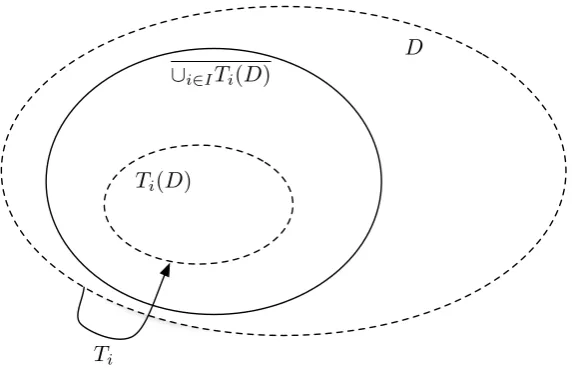
Transfer operators have also been extensively studied on Banach spaces of holo-morphic maps. Less smooth settings have been studied, but the theory of Grothendieck discussed in the next section ensures that the operators will be trace class. Here we have that the transfer operator is a sum of composition operators, multiplied by a weight. So we consider an open, bounded and connected domainD_⊂_Cd, a finite or countable indexing setI, a family of functions (often called inverse branches)_{Ti}i∈I where Ti : D → D is holomorphic, and another family of functions {wi}i∈I with

wi : D→C holomorphic. The transfer operator can be defined on a variety of Ba-nach spaces of holomorphic functions, with the case that Ruelle studied beingF(D). We will also use this space as our setting. The transfer operator _L : F(D)_→F(D) is defined, for f _∈F(D), z _∈Dby

Lf(z) =X i∈I

f(Ti(z))wi(z).

We also require the condition that

[

i∈I

Ti(D)⊂D, (2.7)

in order to get unique fixed points of the inverse branches, and to make sure the operator is ‘analyticity improving’. See figure 2.1.

Ruelle (47) proved that the transfer operator _L is nuclear. Bandtlow and Jenk-inson (5) proved nuclearity for a wide variety of Banach spaces, including F(D). Mayer (33) looked at the case where inverse branches Ti are on an infinite dimen-sional Banach space, and gave technical conditions (including that the derivatives of the branches are nuclear) for the transfer operator to be nuclear.

(31)

D ∪i∈ITi(D)

Ti

[image:31.595.180.467.101.292.2]

Ti(D)

Figure 2.1: The condition _∪i∈ITi(D)⊂D.

M : F(D)_→F(D) given by _Mf(z) =f(T(z))w(z) for f _∈F(D) and z _∈ D. We again require T(D)_⊂D. Let z0 ∈Ddenote the unique fixed point T(z0) = z0. We

have the following formula for the trace,

Tr_M= w(z0) det(I ₋DT(z0))

(2.8)

The formula for Tr_Ln_{is built up using this simpler formula. Fix}_i_{= (}_i

1, . . . , in)∈In. Define Ti =Ti1 ◦Ti2 ◦ · · · ◦Tin, let zi ∈ D be its unique fixed point, and define the map wi : D →C bywi(z) =Qnm=1wim(Tim+1· · ·Tinz). Then the trace formula for Ln _{follows from equation 2.8,}

Tr_Ln =X i∈In

wi(zi) det(I₋DTi(zi))

. (2.9)

Example 2.12. We give an example illustrating the use of the theory in the paper of Jenkinson and Pollicott (23). Let U = B(1/2,3/2), and Ti : U → U, i = 1,2 be given by T1(z) = z/3 and T2(z) = z/3 + 2/3. Define a transfer operator Ls :

(32)

dimension of the middle third Cantor setX, which is the attractor for the IFS given by the two maps T1 and T2, which are inverse branches of the dynamical system

T : X _→X given by T(x) = 3x(mod 1). For transfer operators of this type, there is a maximal real eigenvalue given byeP(−slog|T0|)_{, and if it is 1 then this must mean}

P(₋slog_|T0_|) = 0, and by Bowen’s elegant formula, s is then the dimension of the repeller for T.

In general, X is a compact set in a C∞ manifold which is the attractor for a dynamical system T : X _→X, such that T is expanding, analytic, conformal, and locally maximal, i.e. for a sufficiently small open neighbourhood U of X, we have ∩∞

n=1T

−n_U ₌ _X_{. We also require that the dynamics of} _T _{are coded by a subshift} of finite type. The point of these hypotheses is so that it is always possible to find inverse branches which behave nicely, and can be complexified, so that there is a rich setting to define transfer operators, including being able to use nuclear operator theory. As mentioned in the introduction, the determinant associated with the transfer operator provides the necessary information to find this eigenvalue, and provides a method for a numerical approximation.

Remark 2.13. If_Lt : F(U)→F(U) is a holomorphic family of transfer operators defined by _Ltf(z) =

P

if(Tiz) exp(tw(Tiz)), and µ is aL0-invariant measure, then

there is a nice connection between w and the spectrum of _L0. Let ht ∈ F(U) be the family of eigenvectors corresponding to eigenvaluesλt we get from applying the perturbation theorem with λ0 =h0 = 1. Differentiate Ltht =λtht with respect tot, to get_Lt(h0t+htw) = λ0tht+λtht0. Att = 0, this reduces toL0(h0t|t=0+w) = λ0t|t=0+

h0_t_|t=0. Applying µ, using the L0 invariance, and simplifying gives the equation

Z

wdµ=λ0_t_|t=0.

(33)

Lebesgue measure.

Remark 2.14. Sometimes the weight function is of the form _|w_| where w is a holomorphic function. The imaginary part of_|w_| is always zero, so it cannot satisfy the Cauchy-Riemann equations, so is not holomorphic. However, a trick can be performed, which allows us to use the Grothendieck machinery again. This doesn’t quite come for free because it increases the dimension of the domain we work in, so the convergence of the power series of the determinant isn’t as fast.

Let T : _C_→_C be the underlying transformation. Write

T(x+iy) =T1(x, y) +iT2(x, y),

for x, y _∈ _R, and complexify each of T1 : R2 → R and T2 : R2 → R to get a

function ˜T : _C2 _→

C2 where ˜

T(x1+ix2, y1+iy2) = (T11(x1 +ix2, y1+iy2) +iT12(x1+ix2, y1+iy2),

T21(x1+ix2, y1+iy2) +iT22(x1+ix2, y1 +iy2)).

We have

T11(x1+ 0i, y1 + 0i) = T1(x1, y1)

T12(x1+ 0i, y1 + 0i) = 0

T21(x1+ 0i, y1 + 0i) = T2(x1, y1)

T22(x1+ 0i, y1 + 0i) = 0,

for all x1, y1 ∈ R. These relations tell us derivatives such as ∂T22/∂x1 = 0,

(34)

equations in each variable separately, we may consider the value of the matrix

DT˜(x1+ 0i, y1+ 0i) =



 

∂T˜1

∂x(x1, y1) ∂T˜1

∂y(x1, y1) ∂T˜2

∂x(x1, y1) ∂T˜2

∂y(x1, y1)



 

and using the correspondence between complex numbers and real 2x2 matrices, we get

DT˜(x1, y1) =



 

∂T1

∂x(x1, y1) ∂T1

∂y(x1, y1) ∂T2

∂x(x1, y1) ∂T2

∂y(x1, y1)





,

hence

det(I₋DT˜(x1, y1)) = |1−T0(x1+iy1)|2.

(35)

Chapter 3 Lyapunov Exponents of Random

Matrix Products

3.1 Introduction

Let I be a compact topological space equipped with a probability measure ρ. Con-sider a family of strictly positive non-singular d_×d matrices _{Aα}α∈I, such that each component varies continuously with α.

The Lyapunov exponent λ of this system is defined to be

λ= lim n→∞

1

n

Z

I

Z

I · · ·

Z

I

log_kAα1Aα2· · ·Aαnkdρ(α1)dρ(α2)· · ·dρ(αn). (3.1)

Because the sequence (λn)n∈_N given by

λn =

Z

I · · ·

Z

I

log_kAα1· · ·Aαnkdρ(α1)· · ·dρ(αn)

is easily seen to be sub-additive (λn+m ≤ λn+λm for alln, m ∈N), we may apply the well-known lemma (see for example the book of Walters (61)), to give that

λ _∈ [_−∞,_∞). To exclude the possibility that λ = _−∞, we use that there exists

(36)

3. Lyapunov Exponents of Random Matrix Products 29

constants B >0,C _∈_R such that

kAα1· · ·Aαnk ≥Be

Cn

for alln _∈_Nand allα_∈In_{, which immediately gives}_λ _≥_C_{. To show the inequality,} if the smallest entry of a d_×d matrixAisa, then_kAx_{k ≥ k}x_k1ad1/2 for allx∈Rd+,

where _Rd

+ denotes elements of Rd with strictly positive components. Let aα be the smallest entry for Aα, anda = infα∈Iaα. Each entry in any product Aα1· · ·Aαn is then at least dn−1an. Hence, using that _kA_k = sup_{kAx_k : _kx_k = 1, x _∈ _Rd₊_} for strictly positive A, we have

kAα1· · ·Aαnk ≥ sup

kxk=1k

x_k1d−1/2dnan =BeCn,

for some constants B, C. Showing an upper bound is simpler, since

λn ≤n

Z

I

log_kAαkdρ(α),

for all n, we have λ_≤R_Ilog_kAαkdρ(α).

Consider the case where I =_{1, . . . , m_} is equipped with the discrete topology, and ρis a probability measure on I, so is given by ρ=Pm

i=1piδi where eachpi ≥0,

p1+· · ·+pn = 1, and δi is the Dirac delta function at i, i.e. δi(A) = χA(i). Then equation 3.1 becomes

λ= lim n→∞

1

n

X

i∈In

pi1pi2· · ·pinlogkAi1Ai2· · ·Aink,

(37)

We would like to recast the quantity λas something involving a suitably defined transfer operator, to find a new expression for the Lyapunov exponent. We can then invoke the tools of Grothendieck and write the Lyapunov exponent in terms of the determinant, involving periodic points of the transformations used to define the transfer operator.

Transfer operators sum or integrate over a family of composition operators. The tools for calculating the trace of these transfer operators rely heavily on complex analysis. We therefore need to study a family of maps which encode spectral in-formation about the matrices, and are nice from a complex analysis point of view. These maps are the multi-dimensional linear fractional transformations, which are used in the study of multi-dimensional continued fractions.

First note that if we set

A0_α =aαAα

whereaα is some scaling variable which depends continuously onα then we see that the Lyapunov exponent λ0 of this family is

λ0 = lim n→∞

1

n

Z

I

Z

I· · ·

Z

I

log_kAα1Aα2· · ·Aαnk

+ n

X

i=1

log_|aαi|dρ(α1)dρ(α2)· · ·dρ(αn) = λ+

Z

I

log_|aα|dρ(α),

(38)

[image:38.595.198.451.100.332.2]

Figure 3.1: z _∼ z0 and w _∼w0 because the lines which connect them pass through the origin.

3.2 A Family of Maps

We first examine the manifold _CPd−1, the complex projective space, and show that it naturally gives rise to the linear fractional transformation associated with a matrix

Aα.

For 0 ₆= z, w _∈ _Cd_{, we say that} _z _∼ _w _{if there exists} _λ _∈

C such that z = λw, see figure 3.1. We write [z] =_{w_∈_Cd _: _w_∼_z_}_{, and define}

CPd−1 as the quotient space

CPd−1 = (Cd− {0})/∼={[z] : z ∈Cd− {0}}.

We equip it with the quotient topology, that is defining π : _Cd _→ _CPd−1 by

πz = [z], we declare πU to be open in _CPd−1 whenever U _⊂ _Cd is open. For readability [z1, . . . , zd] is understood to mean [(z1, . . . , zd)].

(39)

Ui ={[z1, . . . , zd] : zi 6= 0} and then maps φi : Ui →Cd−1− {0} by

φi[z1, . . . , zd] =zi−1(z1, . . . , zi−1, zi+1, . . . , zd).

The setsUi coverCPd−1, and that the mapsφi are well defined bijections. We show that they are homeomorphisms. LetU _⊂_Cd−1_{− {}₀_} _{be open. Then}_φ−1

i (U) is open because V = _{0 ₆= (z1, . . . , zd) ∈ Cd : zi−1(z1, . . . , zi−1, zi+1, . . . , zd) ∈ U} is open in _Cd_{, since} _πV ₌ _φ−1

i (U). Let U ⊂ CPd

−1 _{be open. So} _U ₌ _πV _{for some open}

V _⊂ _Cd, and φi(U) = φi(πV) = {zi−1(z1, . . . , zi−1, zi+1, . . . , zd) : (z1, . . . , zd) ∈ V}, which is open. Hence φj(U) is open in Cd−1.

For the inverse, we can write

φ−_i 1(z1, . . . , zd−1) = [z1, . . . , zi−1,1, zi+1, . . . , zd−1],

and then see that the co-ordinate change functionsφi◦φ−j1 : Cd−1−{0} →Cd−1−{0} are holomorphic.

So _CPd−1 _{is a complex manifold of dimension} _d₋_{1. We are interested in an}

open sub-manifold. Let _R+ denote the strictly positive reals. We embed Rd+ in Cd

in the obvious way. Define an open set

Q=_{(z1, . . . , zd) : zj =xj +iyj ∈C, xj, yj >0, j = 1, . . . , d}=Rd++iR

d

+,

soπQgives an open sub-manifold which we callM. The family of positive matrices (Aα)α∈I act naturally on this manifold. We may define functions

Aα : M →M; Aα([z1, . . . , zd]) = [Aα(z1, . . . , zd)].

Since Aαλz = λAαz when z ∈ Cd and λ ∈ C, and since it is readily seen that

(40)

Note that M _⊂Ui for each i, so an atlas for M need only contain one map, so we may define

φ :M _→_Cd−1; φ[z1, . . . , zd] =z1−1(z2, . . . , zd),

which is injective, so we’d like to know what the imageφ(M) is. Ifw= (w1, . . . , wd−1) =

φ([r1eiθ1, . . . , rdeiθd]) for some ri > 0 and θi ∈ (0, π/2) for each i = 1, . . . , d, then argwj = θj+1−θ1 ∈(−π/2, π/2) and argwi−argwj =θi+1−θj+1 ∈(−π/2, π/2).

These conditions are equivalent to Rewj >0 and Rewiwj >0. Define

D =_{(z1, . . . , zd−1)∈Cd−1 : Rezi >0 and min

i6=j Rezizj >0}

and let (w1, . . . , wd−1)∈D. Let θ =−miniargwi+for some small >0. If θ >0 then set instead θ =. Set z =eiθ(1, z1, . . . , zd−1). We have that [z]∈M and that

any other pre-image is equal to [z]. So henceforth we writeφ :M _→D, upgrading

φ to a bijection.

The set D is open, convex, and contains the positive real axis

Rd+−1 ={z ∈Cd

−1 _: _Re_z

i >0, Imzi = 0}. (3.2)

This suggests there are links with the complex cones of Rugh, see (50) for example, in which case far more could be said of the maps we define on this set.

The maps φ_◦Aα◦φ−1 : D →D have simple expressions and are holomorphic in each variable separately by the algebra of holomorphic functions.

Definition 3.1. For α_∈I, we define the mapTα : D →D by

(41)

To be explicit, if Aα has entriesa

(α)

ij , for z = (z1, . . . , zd−1) we can write

Tα(z) =

a₂₁(α)+a₂₂(α)z1+· · ·+a (α) 2d zd−1

a₁₁(α)+a₁₂(α)z1+· · ·+a (α) 1d zd−1

, . . . ,a

(α)

d1 +a (α)

d2 z1+· · ·+a (α)

dd zd−1

a₁₁(α)+a₁₂(α)z1+· · ·+a (α) 1dzd−1

!

.

For α_∈In we define Tα =Tα1 ◦ · · · ◦Tαn.

We remark that in looking at this expression directly, it may not be immediately clear that it maps D_→D. These maps have useful properties and correspond well with the original matrices, and similar maps are used in multidimensional continued fraction theory, see the book of Schweiger (54). Similar maps can be used to prove the Perron-Frobenius theorem for finite matrices (see (2) for a proof), but this variation is so that the maps are holomorphic.

It is sometimes useful to define the linear fractional transformation for an arbi-traryd_×d matrix B, not just ones with positive entries. Where it makes sense, we define TB : Cd−1 →Cd−1 by

TB(z) =

A2·z˜

A1·z˜

, . . . ,Ad·z˜ A1·z˜

,

where Ai is the vector given by the ith row of the matrix B, and ˜z is the vector in Cd given by (1, z1, . . . , zd−1).

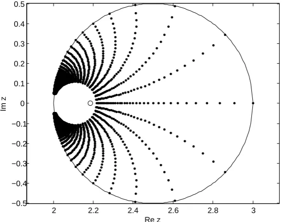
Example 3.2. We consider the complex linear fractional transformation associated with the positive 2_×2 matrix (a b

c d). The transformation is then the mapT : D→D where D=_{z _∈_C : Rez >0_} given by

T(z) = c+dz

a+bz.

The boundary of the image T(D) consists of pointsT(is) for s_∈_R(where we have extended the domain of T to include points on the imaginary axis).

(42)

2 2.2 2.4 2.6 2.8 3

−0.5 −0.4 −0.3 −0.2 −0.1 0 0.1 0.2 0.3 0.4 0.5

Re z

[image:42.595.170.460.96.324.2]

Im z

Figure 3.2: A plot of T(z) for various (regularly spaced) z _∈ D for a 2_×2 matrix in example 3.2. The small circle at z = 2.18 is the fixed point.

T, finding s2 in terms of xand substituting into y2, we arrive at

x₋ bc+ad

2ab

2

+y2 = (bc−ad)

2

4a2_b2 ,

so T(D) is always the interior of a circle centred on the real axis, and contained entirely in the positive imaginary half of the complex plane. In figure 3.2, we plot the images of regularly spaced points in [0,1.8]+i[₋10,10] _⊂Dfor the matrix (1 2

3 4),

and include the bounding circle, and the fixed point.

We now need to state and prove some important properties of these maps before we employ them to define transfer operators.

Lemma 3.3. For allα _∈I, the mapTα associated with the matrix Aα has Tα(D)⊂

D. In fact,

∪α∈ITα(D)⊂D (3.3)

and this set is compact in D.

(43)

of (d _×d)-dimensional positive matrices _{Aα}α∈I where I is a compact set, and the entry for the ith row and jth column of Aα is denoted by a

(α)

ij . We show this by induction on d. For d = 2, _kTαk∞ = max(|a(₁₁α)/a₂₁(α)|,|a₁₂(α)/a(₂₂α)|) by a routine

calculation, and this right hand side is uniformly bounded because it is a continuous function of α on a compact set. This establishes the basis for the induction.

Assume now d > 2, and the result holds for d₋1. If the result does not hold for d, there exists a sequence (yn)n∈N in ∪αTα(D) where yn = Tαn(xn) for some sequences (xn)n∈Nand (αn)n∈N inDand I respectively, where some componentj of

yn is unbounded. Write

y_n(j) = An+a

(αn) jd x

(d−1)

n

Bn+a

(αn)

1d x

(d−1)

n

where An=a

(αn) j1 +a

(αn) j2 x

(1)

n +· · ·+a(_jα₍_dn₋)₁₎x(nd−2) and Bn=a

(αn)

11 +a (αn)

12 x (1)

n +· · ·+

a(αn)

1(d−1)x (d−2)

n . Hence y(nj) = fn(x

(d−1)

n ) where fn : D → C is defined by fn(x) = (An +a

(αn)

jd x)/(Bn+a

(αn)

1d x). But kfnk∞ ≤ max{|An|/|Bn|,|a

(αn) jd |/|a

(αn)

1d |}. Since

An/Bn looks like a fractional transformation of a (d − 1)×(d − 1)-dimensional family, by induction it is bounded, by M say. Also α _{7→ |}a(_jdα)_|/_|a(₁α_d)_| is a continuous function on a compact spaceI, hence bounded. Hence (fn)n∈Nis uniformly bounded,

and therefore so is y(nj), a contradiction.

We next show that _∪α∈ITα(D) ⊂ D. Let zn ∈ ∪α∈ITα(D) such that zn → z for some z _∈ D. Since Tα(D) = φ ◦Aα ◦ φ−1(D) = φ◦ Aα(M), we may write

zn = φ(Aαn(wn)) where wn ∈ M. Write wn = [xn+iyn] where xn, yn ∈ R d

+ have

positive co-ordinates. Picking a component j of zn, we see that

z_n(j) = A

(αn)

j+1 ·xn+iA

(αn) j+1 ·yn

A(αn)

1 ·xn+iA

(αn)

1 ·yn

(44)

where A(αn)

i is the vector given by the ith row of Aαn, and hence

Rez_n(j) = (A

(αn)

j+1 ·xn)(A

(αn)

1 ·xn) + (A

(αn)

j+1 ·yn)(A

(αn)

1 ·yn) (A(αn)

1 ·xn)2+ (A

(αn)

1 ·yn)2 ≥ (minia

(αn)

j+1,i)(minia

(αn)

1,i )(kxnk12+kynk21)

kA(αn)

1 k2(kxnk2+kynk2) ≥ (minia

(αn)

j+1,i)(minia

(αn)

1,i )k2 kA(αn)

1 k2

≥B,

whereB >0 does not depend onn, and the second to last inequality is because_{k · k} and _{k · k}1 are equivalent norms givingk · k1 ≥kk · k. The last inequality is because

α _7→ (minia

(α)

j+1,i)(minia

(α) 1,i)/kA

(α)

1 k2 is a strictly positive continuous function on a

compact set, hence its minimum B is strictly positive. Therefore Relimn→∞zn(j) ≥

B >0.

It only remains to show that for any components i, j we have Rez(i)_z(j) _> _0.

This works in a very similar fashion to the previous paragraph, and we use the same notation.

Rez(i)z(j) ₌ Re(A (αn)

i+1 ·wn)(A

(αn) j+1 ·wn) |A(αn)

1 ·wn|2 ≥ (minka

(αn)

i+1,k)(minka

(αn)

j+1,k)(kxnk

2

1+kynk21)

kA(αn)

1 k2(kxnk2+kynk2)

≥B >0.

This completes the proof that z _∈D.

The fixed points ofTαtell us the eigenvectors ofAαand vice versa. The derivative ofTα evaluated at the fixed point tells us about the spectral radius ofAα. The next lemma gives the details of these relationships. We anticipate this result is already in the literature about linear fractional transformations, but have not been able to find a reference.

Lemma 3.4. Fix any α _∈ I, and let λα be the maximal positive eigenvalue for Aα

by the Perron-Frobenius Theorem. Let Xα = (X

(1)

(45)

eigenvector. Then xα = (X

(2)

α /Xα(1), . . . , Xα(d)/Xα(1)) is the unique fixed point ofTα.

We can recover information about the maximal eigenvalue from the fractional

transformation using the formula

λα =

detAα detDTα(xα)

1_d

Proof. We have

Tα(xα) =

a(₂₁α)Xα(1)+· · ·+a(₂α_d)Xα(d)

a(₁₁α)Xα(1)+· · ·+a(₁α_d)Xα(d)

, . . . , a

(α)

d1 X (1)

α +· · ·+a(_ddα)Xα(d)

a(₁₁α)Xα(1)+· · ·+a(₁α_d)Xα(d)

!

=

(AαXα)2

(AαXα)1

, . . . , (AαXα)d

(AαXα)1

=

λαX2

λαX1

, . . . ,λαXd λαX1

=xα.

That it is unique follows from a version (55) of the Perron-Frobenius theorem which tells us that the only positive eigenvector is the one corresponding to the maximal positive eigenvalue. This gives uniqueness because if y is another fixed point, then (1, y1, . . . , yd−1) would be another positive eigenvector.

To prove the formula for the eigenvalue, we fix α and writeAα=QJ Q−1 where

J is the block Jordan form matrix for Aα and Q is the associated change of basis matrix. This decomposition is not unique, because we can re-order the blocks in J

and this permutes columns of Q. Consider the term TQ−1(x_α). If the first column

of Q isXα, we have

TQ−1(x_α) = φ◦Q−1◦φ−1(x_α) =φ(X_α(1)Q−1(X_α)) = (0, . . . ,0),

and if Xα is not the first column of Q then the term is undefined. Since this term occurs in the subsequent equations, we require that the ordering of the decompo-sition has Xα as the first column, and therefore has λα as the first element of the Jordon block. The rest of the ordering does not matter.

(46)

hence

DTα(xα) = D(TQ◦TJ ◦TQ−1)(x_α)

= DTQ(TJ ◦TQ−1x_α)DT_J(T_Q−1x_α)DT_Q−1(x_α)

= DTQ(TQ−1xα)DT_J(T_Q−1xα)DT_Q−1(xα),

and taking the determinant, rearranging, then unapplying the chain rule for Jaco-bians, we have

detDTα(xα) = det(DTQ(TQ−1x_α)DT_Q−1(x_α)) detDT_J(T_Q−1x_α)

= detDTJ(TQ−1x_α).

We denote the diagonal of J as (λ1, . . . , λd) with λ1 = λα and the upper diagonal as (ρ1, . . . , ρd−1) with each ρi equalling 0 or 1. Sinceλ1 is in a 1×1 block, ρ1 = 0.

A calculation gives that detDTJ(TQ−1x_α) = λ −(d−1) 1

Qd

i=2λi. Hence we have

detAα detDTα(xα)

1_d

=

detJ

detDTJ(TQ−1x_α) 1_d

=

Qd

i=1λi

λ−₁(d−1)Qd

i=2λi

!1_d

=λ1,

completing the proof.

Note that the previous lemma also works for α _∈In in place ofα _∈I.

If we restrict our attention to the family (Tα)α∈I on a suitable compact set, which contains the fixed points, then we retain information about the spectral radii of the matrices. We first need a standard result from point set topology.

Lemma 3.5. LetF be a compact set, and U be open, such that F _⊂U. Then there exists an open bounded set V such that F _⊂ V and V _⊂ U. In addition if U is convex then V can be made to be convex.

(47)

Rudin (46), which applies to any locally compact Hausdorff topological space. This gives us an open bounded set V satisfying F _⊂ V _⊂ V _⊂ U. To obtain convexity, we replaceV by its convex closureV0. This is still open, and certainlyF _⊂V0 _⊂U. If x _∈ V0 then x = limn→∞tnan+ (1−tn)bn with tn ∈ [0,1], an ∈ V, and bn ∈ V. We may pass to subsequences to assume tn → t ∈ [0,1], an → a ∈ V ⊂ U and

bn → b ∈ V ⊂ U. Hence x = ta+ (1− t)b, and since U is convex, x ∈ U, so

V0 _⊂U.

The convexity ensures that the sets this lemma produces are connected. Now ∪α∈ITα(D) is compact by lemma 3.3. So apply lemma 3.5, to get an open, bounded, connected set U such that _∪α∈ITα(D) ⊂ U ⊂ U ⊂ D. Now we have ∪α∈ITα(U) ⊂ ∪α∈ITα(D) ⊂ U, so we can now take the maps Tα to be defined Tα : U → U. Note that U still contains all of the fixed points, because if Tαxα = xα then xα ∈ ∪α∈ITα(D) ⊂ U. Because D is a large set, we have a large choice for the set U. It might be possible to simplify subsequent work by choosing it to be a suitable polydisc. This is certainly possible for 2_×2 matrices.

Lemma 3.6. There exists an >0 such that _kTα(x)₋y_{k ≥} for all α_∈I, x_∈U

and y_∈_Cd−1_\_U_.

Proof. Set K = _∪α∈ITαU which is compact by lemma 3.3, and K ⊂ U. For each

x _∈ K, there exists δx > 0 such that B(x,2δx) ⊂ U. The compactness of K gives the existence of a finite subset _{x1, . . . , xN} ⊂ K such that K ⊂ ∪Ni=1B(xi, δxi). Fix x _∈ U, α _∈ I, y _∈ _Cd−1 _\_U_. _T

α(x) ∈ K so Tα(x) ∈ B(xi, δxi) for some i.

y /_∈B(xi,2δxi) so 2δxi ≤ kxi−yk ≤ kxi−Tα(x)k+kTα(x)−yk ≤δxi+kTα(x)−yk implying δxi ≤ kTα(x) − yk. The proof of this lemma is completed by setting

= min_{δxi|i= 1, . . . , N}.

(48)

We will also require a suitable metric which makes _{Tα}α∈I a family of uniform contractions.

Lemma 3.7. There exists a metric d on U, and a constant 0< k <1 such that

d(Tαx, Tαy)≤kd(x, y) (3.4)

for all α_∈I and all x, y _∈D. There exists a constant m >0 such that

kx₋y_{k ≤}md(x, y) (3.5)

for all x, y _∈ U. (As usual _{k · k} is the Euclidean norm in _Cd−1). For each x _∈ U, there exists a constant r >0 and a constant Mx >0 such that

d(x, y)_≤Mxkx−yk (3.6)

for all y_∈Bd(x, r).

Proof. The metric is the Carath´eodory-Reiffen Finsler metric used in the paper (10) of Earle and Hamilton to prove their fixed point theorem. We give an outline of the construction used in the paper, and add in detail to show the uniformity of the contraction constant for our maps, and the existence of the local bound to the Euclidean metric.

Let H∞(U) denote the bounded holomorphic functions on U. Define

α(x, v) = sup_{kDf(x)v_k : _kf_k∞ ≤1, f ∈H∞(U)}

for allx_∈U andv _∈_Cd−1_{. Let Γ denote the set of curves [0}_,_1]_→_U _{with piecewise}

continuous derivatives. For γ _∈Γ, set

Lα(γ) =

Z 1

0