Subspace Learning from Image Gradient
Orientations
Georgios Tzimiropoulos,
Member, IEEE,
Stefanos Zafeiriou
Member, IEEE,
and Maja Pantic
Fellow, IEEE
Abstract—We introduce the notion of subspace learning from image gradient orientations for appearance-based object recognition. As image data is typically noisy and noise is substantially different from Gaussian, traditional subspace learning from pixel intensities fails very often to estimate reliably the low-dimensional subspace of a given data population. We show that replacing pixel intensities with gradient orientations and the2norm with a cosine-based distance measure offers, to some extend, a remedy to this problem. Within this framework, which we coin IGO (Image Gradient Orientations) subspace learning, we first formulate and study the properties of Principal Component Analysis of image gradient orientations (IGO-PCA). We then show its connection to previously proposed robust PCA techniques both theoretically and experimentally. Finally, we derive a number of other popular subspace learning techniques, namely Linear Discriminant Analysis (LDA), Locally Linear Embedding (LLE) and Laplacian Eigenmaps (LE). Experimental results show that our algorithms outperform significantly popular methods such as Gabor features and Local Binary Patterns and achieve state-of-the-art performance for difficult problems such as illumination- and occlusion-robust face recognition. In addition to this, the proposed IGO-methods require the eigen-decomposition of simple covariance matrices and are as computationally efficient as their corresponding 2 norm intensity-based counterparts. Matlab code for the methods presented in this paper can be found at http://ibug.doc.ic.ac.uk/resources.
Index Terms—image gradient orientations, robust principal component analysis, discriminant analysis, non-linear dimensionality reduction, face recognition
✦
1
I
NTRODUCTIONS
UBSPACE learning for computer vision applications has recently attracted a lot of interest in the scientific community [1], [2], [3], [4], [5], [6], [7], [8], [9], [10], [11], [12], [13], [14], [15]. This research has been primarily motivated by the development of a multitude of tech-niques for the efficient analysis of high-dimensional data via non-linear dimensionality reduction [3], [4], [5], [6], [10], [13]. These techniques have provided valuable tools for understanding and capturing the intrinsic non-linear structure of visual data encountered in many important machine vision problems. At the same time, there has been a substantially increasing interest in related appli-cations such as appearance-based object/face recognition and image retrieval.Scientific efforts in the field have mainly revolved around two lines of research. Kernel-based methods
• The research presented in this paper has been funded by the European
Research Council under the ERC Starting Grant agreement no. ERC-2007-StG-203143 (MAHNOB). The work by G. Tzimiropoulos is currently sup-ported in part by the European Communitys 7th Framework Programme [FP7/2007-2013] under grant agreement no. 288235 (FROG). The work of S. Zafeiriou was funded in part by the Junior Research Fellowship of Imperial College London.
G. Tzimiropoulos is with the School of Computer Science, University of Lincoln, LN6 7TS, U.K. He is also with the Department of Com-puting, Imperial College London, SW7 2AZ, U.K. (e-mail: [email protected]).
S. Zafeiriou is with the Department of Computing, Imperial College London, SW7 2AZ, U.K. (e-mail: [email protected]).
M. Pantic is with the Department of Computing, Imperial College Lon-don, SW7 2AZ, U.K. She is also with the Department of Computer Science, University of Twente, Enschede 7522 NB, the Netherlands (e-mail: [email protected]).
extend linear subspace analysis, such as Principal Com-ponent Analysis (PCA) and Linear Discriminant Analy-sis (LDA), in arbitrary dimensional Hilbert spaces [16], [5], [6], [17], [10], [18], [13]. These methods perform an implicit mapping of input data into a high-dimensional Hilbert space (also referred to as feature space) where efficient representations are obtained through linear sub-space analysis, while all computations are efficiently performed via the inner product of the feature space (the so-called kernel trick). Manifold learning algorithms [1], [2], [3], [4], [19], [7], [11], [12] assume that input data points are actually samples from a low-dimensional manifold embedded in a high-dimensional space. This assumption is not unreasonable in computer vision where large amounts of collected data often result from changes in very few degrees of freedom. This, in turn, attributes input data with a well-defined and probably predictable structure. Manifold learning methods per-form dimensionality reduction with the goal of finding this underlying structure. This is typically performed by preserving local neighborhood information in a certain sense. Typical examples include Isomap [2], Locally Lin-ear Embedding (LLE) [1], [4] and Laplacian Eigenmaps (LE) [3].
A fundamental problem of the majority of subspace learning techniques (both linear and non-linear) for appearance-based object recognition is that they are not robust. Most methods are usually based on linear correlation of pixel intensities (for example [20], [21], [7]) which fails very often to model reliably visual sim-ilarities/correlations. For example, Eigenfaces [20] uses Principal Component Analysis (PCA) of pixel intensities
to estimate the K−rank linear subspace of a set of training face images by minimizing the 2 norm. The
solution, given by the eigen-analysis of the training data covariance matrix, enjoys optimality properties only when noise is i.i.d. Gaussian; for data corrupted by outliers, such as occlusions, illumination changes and cast shadows, the estimated subspace can be arbitrarily biased.
In this paper, to remedy (at least to some extend) this problem, we introduce a new framework for appearance-based object recognition: subspace learning from image gradient orientations (IGO subspace learning). We pro-pose a class of IGO-algorithms whichdo not operate on pixel intensities but use gradient orientations and replace linear correlation of pixel intensities with the cosine of gradient orientation differences. We formalize and statistically verify the observation that local orientation mismatches caused by outliers can be well-described by a uniform distribution which, under a number of mild assumptions, is cancelled out when the cosine kernel is applied. This last observation has been noticed in recently proposed schemes for image registration [22] and provides the basis for a robust measure of visual correlation.
Based on this line of research, we show that a cosine-based distance measure has a functional form which en-ables us to define an explicit mapping from the space of gradient orientations into a subset of a high-dimensional sphere where essentially linear or non-linear dimension-ality reduction is performed. Then, we formulate and study the properties of PCA of image gradient orien-tations (IGO-PCA) and show its connection to previ-ously proposed robust PCA techniques both theoretically and experimentally. Next, we derive a number of other popular subspace learning techniques, namely Linear Discriminant Analysis (LDA), Locally Linear Embed-ding (LLE) and Laplacian Eigenmaps (LE). Similarly to previous work on dimensionality reduction, the basic computational module of the IGO-algorithms requires the eigen-decomposition of simple covariance matrices, while high dimensional data can be efficiently analyzed following the strategy suggested in [20].
Our work and contributions in this paper are summa-rized as follows. In Section 2, we define and statistically verify a notion of pixel-wise image dissimilarity by look-ing at the distribution of gradient orientation differences. This provides the intuition and the basis for measuring image correlation using the cosine of gradient orientation differences as explained in the first part of Section 3. The remaining of this section describes the key points for IGO subspace learning and introduces our IGO-PCA. This section concludes with a theoretical analysis which shows the connection of IGO-PCA to the general M-estimation framework of [23] for robust PCA. In Section 4, we evaluate the robust properties of IGO-PCA for the applications of face reconstruction and recognition and present comparisons with previously proposed methods. In Section 5, we study LDA, LLE and LE within the
proposed IGO-framework. In Section 6, we present face recognition experiments on the extended Yale B, PIE, FERET and AR databases. Our results show that our al-gorithms outperform significantly popular methods such as Gabor features and Local Binary Patterns and achieve state-of-the-art performance for difficult problems such as illumination- and occlusion-robust face recognition. In Section 7, we propose an efficient and exact online version of our IGO-PCA and show how this algorithm can boost the performance of appearance-based tracking. Section 8 concludes the paper. Finally, Matlab code for the methods presented in this paper can be found at http://ibug.doc.ic.ac.uk/resources.
2
R
ANDOM NUMBER GENERATION FROM IM-AGE GRADIENT ORIENTATION DIFFERENCES
Before describing our contributions, we have to define some useful notation. S, {.} denotes a set, examples include which is the set of reals and C is the set of complex numbers.x,xandXdenote a scalar or a com-plex number, a column vector and a matrix, respectively. Re[x] and Im[x] are the real and imaginary part of x, respectively.x(k)is the k-th element of vector x,N(X)
is the cardinality of set X and Nx number of neighbors ofx.Im×mis them×midentity matrix and1is vector or
matrix of ones.||.||and||.||F denote the2and Frobenius
norm, respectively.X∗andXHare the conjugate and the conjugate transpose of X, respectively. Finally,U[a, b] is a uniform distribution in [a, b], E[.] is the mean value operator andx∼U[a, b]means thatxfollowsU[a, b].
Central to the IGO-methods is the distribution of im-age gradient orientation differences and the cosine kernel which provide us a consistent way to measure image correlation/similarity when image data is corrupted by outliers. In this section, we formalize an observation for the distribution of gradient orientation differences and describe an experiment which verifies the validity of our argument. In the next section, we will assume that, for data corrupted by outliers, the corresponding distribution will also have this well-defined structure.
Consider a set of images {Ji},Ji ∈ m1×m2. At each
pixel location, we estimate the image gradients and the corresponding gradient orientation 1. We denote by
{Φi},Φi ∈ [0,2π)m1×m2 the set of orientation images
and compute the orientation difference image
ΔΦij =Φi−Φj. (1)
We denote by P the set of indices corresponding to the image support and by φi and Δφij φi − φj the N(P)−dimensional vectors obtained by writing Φi and ΔΦij in lexicographic ordering. We introduce the
1. More specifically, we compute Φi = arctanGi,y/Gi,x, where
following definition.
Definition I. Images Ji and Jj are pixel-wise dissimilar
if ∀k∈ P,Δφij(k)∼U[0,2π).
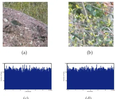
Not surprisingly, nature is replete with images exem-plifying Definition I. This, in turn, makes it possible to set up a naive image-based random number generator. To confirm this, we used more than70,000pairs of image patches of resolution200×200randomly extracted from natural images [24]. For each pair, we computed Δφij and formulated the following null hypothesis
• H0:∀k∈ P Δφij(k)∼U[0,2π)
which was tested using the Kolmogorov-Smirnov test [25]. For a significance level equal to 0.01, the null
hy-pothesis was accepted for94.05%of the image pairs with mean p-value equal to 0.2848. In a similar setting, we
tested Matlab’s random generator. The null hypothesis was accepted for 99.48% of the cases with mean p -value equal to 0.501. Fig. 1 (a)-(b) show a typical pair of
image patches considered in our experiment. Fig. 1 (c) and (d) plot the histograms of the gradient orientation differences and 40,000 samples drawn from Matlab’s random number generator respectively.
(a) (b)
0 1 2 3 4 5 6.2832
0 50 100 150
Δ Φ(radius)
Number of Pixels
(c)
0 1 2 3 4 5 6.2832
0 50 100 150
ΔΦ(radius)
Number of Pixels
[image:3.612.333.558.256.324.2](d)
Fig. 1. (a)-(b) An image pair used in our experiment, (c) Image-based random number generator: histogram of 40,000 gradient orientation differences and (d) Histogram of 40,000 samples drawn from Matlab’s random number generator.
3
IGO-PCA
3.1 Cosine-based correlation of image gradient ori-entations
Assume that we are given a set of n images {Ii},Ii ∈ m1×m2 with the goal of subspace learning for
appearance-based object recognition. We compute the corresponding set of orientation images {Φi} and mea-sure image correlation using the cosine kernel [22], [26]
s(φi,φj)
k∈P
cos[Δφij(k)] =cN(P) (2)
where c ∈ [−1,1] and k is the pixel index. Notice that for highly spatially correlated images Δφij(k) ≈0 and
c→1.
Assume that there exists a subset P2 ⊂ P
corre-sponding to the set of pixels corrupted by outliers. For P1=P − P2, we have
s1(φi,φj) =
k∈P1
cos[Δφij(k)] =c1N(P1) (3)
wherec1∈[−1,1].
Not unreasonably, we assume that in P2 the images
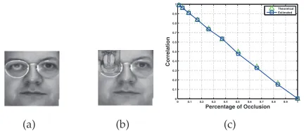
are pixel-wise dissimilar according to Definition I. For example, Fig. 2 (a)-(b) show an image pair where P2
is the part of the face occluded by the scarf. Fig. 2 (c) plots the distribution ofΔφinP2. Before proceeding for
(a) (b)
0 1 2 3 4 5 6.2832
0 5 10 15 20 25
ΔΦ (radius)
(c)
Fig. 2. (a)-(b) An image pair used in our experiments. (c) The distribution ofΔφfor the part of the face occluded by the scarf.
computing the value of s in P2, we need the following
theorem [22] (please refer to Section I of supplementary material for a proof).
Theorem I Let u(.) be a random process and u(t) ∼
U[0,2π)then:
• E[Xcosu(t)dt] = 0for any non-empty intervalX ∈ R.
• Ifu(.)is mean ergodic, then Xcosu(t)dt= 0.
We also make use of the following approximation
Xcos[Δφij(t)]dt∝
k∈P
cos[Δφij(k)] (4)
where with some abuse of notation, Δφij is defined in the continuous domain on the left hand side of (4). Analogously, the above hold for the case of the sine kernel as well.
Based on the above results, forP2, we have
s2(φi,φj) =
k∈P2
cos[Δφij(k)]0. (5)
Overall, unlike 2-based correlation of image
inten-sities where the contribution of outliers can be arbi-trarily large, s(.) measures correlation as s(φi,φj) = s1(φi,φj)+s2(φi,φj)c1N(P1), i.e. the effect of outliers
is approximately canceled out 2.
To exemplify the above concept, we considered the following experiment. We calculated sfrom face image
[image:3.612.78.269.350.515.2]pairs where the second image was directly obtained from
the first one after applying a synthetic occlusion with a
“Baboon” patch of increasing size. Fig. 3 (a) and (b) show an example of image pairs considered. Note that, for all image pairs, we are guaranteed that c1 = 1 and, given
that the above analysis holds, we also have s1=N(P1)
(the image P1 is exactly the same in both images)
and hence s ≈ N(P1). Under the assumption that the
gradient orientation differences of dissimilar objects are uniformly distributed, then s2 ≈0. If s2 was exactly 0
then s = N(P1) would be the number of pixels that
have not been occluded. If s is normalized by the total number of pixels N(P) then the correlation coefficient
s/N(P) would be the percentage of the image that has not been occluded. Fig. 3 (c) shows both the theoretical value of s/N(P), which is N(P1)/N(P), as well as, its
value as estimated from the data as a function of the percentage of the occlusion (the percentage of occlusion is N(P2)/N(P)). As we may observe, the difference
between the theoretical and estimated values is almost negligible.
(a) (b)
0 0.1 0.2 0.3 0.4 0.5 0.6 0.7 0.8 0.9 1
0 0.1 0.2 0.3 0.4 0.5 0.6 0.7 0.8 0.9 1
Correlation
Percentage of Occlusion
Theoretical Estimated
[image:4.612.67.283.345.438.2](c)
Fig. 3. Cosine-based correlation of image gradient orien-tation for the case of synthetic occlusions. (a)-(b) A pair of images considered for our experiment. (c) Theoretical and expected values of s/N(P) as a function of the percentage of occlusionN(P2)/N(P).
3.2 The principal components of image gradient ori-entations
To show how (2) can be used as the basis for our IGO-PCA, we first define the distance
d2(φi,φj)
k∈P
1−cos[Δφij(k)]) (6)
We can write (6) as follows
d2(φi,φj) = 12
k∈P
2−2 cos[φi(k)−φj(k)]
= 1
2
k∈P
(cos2φ
i(k) + sin2φi(k))
+(cos2φ
j(k) + sin2φj(k))
−2(cosφi(k) cosφj(k)
+ sinφi(k) sinφj(k))
= 1
2
k∈P
(cosφi(k)−cosφj(k))2
+(sinφi(k)−sinφj(k))2
= 1
2ejφi−ejφj
2
(7)
where ejφi = [ejφ1, . . . , ejφN(P)]T. The last equality
makes the basic computational module of our scheme apparent. We define the mapping from [0,2π)p onto a subset of complex sphere with radiusN(P)3
zi(φi) =ejφi (8)
and apply complex linear PCA to the transformed data
zi. That is, we look for a set of K < n orthonormal bases U = [u1| · · · |uK] ∈ CN(P)×K by minimizing the error function
(U) =||Z−UUHZ||2F (9)
where Z = [z1| · · · |zn] ∈ CN(P)×n and, without loss of generality, we assume zero-mean data. Equivalently, we can solve
Uo = arg maxUtr UHZZHU
subject to (s.t.) UHU=I. (10)
The solution is given by theK-th eigenvectors of ZZH corresponding to the K-th largest eigenvalues. Finally, theK−dimensional embeddingC= [c1| · · · |cn]∈ CK×n ofZ are given byC=UHZ.
Using the results of the previous subsection, we can remark the following.
Remark I.IfP =P1∪ P2 withΔφij(k)∼U[0,2π) ∀k∈
P2, then Re[zHi zj]c1N(P1)
Remark II.IfP2=P, then Re[zHi zj]0and Im[zHi zj]
0.
Further geometric intuition about the mapping zi is
provided by the chord between vectorszi and zj
crd(zi,zj) =
(zi−zj)H(zi−zj) =
2d2(φi,φj) (11)
Using crd(.), the results of Remark I and II can be
re-formulated as crd(zi,zj)
2((1−c1)N(P1) +N(P2))
and crd(zi,zj)2N(P)respectively.
Let us denote by Q = {1, . . . , n} the set of image indices and Qi any subset of Q. Let us also denote by Λthe positive eigen-spectrum ofZZH. We can conclude
the following
Remark III. If Q = Q1∪ Q2 with zHi zj 0 ∀i ∈ Q2,
∀j ∈ Q and i = j, then, ∃ eigenvector ul of Un such
that ul N(1P)zi. In Remark III, we assume that the data population Q can be written as a union of two disjoint subsets. The samples belonging to subset Q1
are not orthogonal to each other. This subset could be for example a collection of face images. Q2 denotes
the samples which are all (approximately) orthogonal to each other and are all (approximately) orthogonal to each of the samples of Q1. Soj can either belong toQ1 or to
Q2, that is could be any sample of Q. The subset Q2
is supposed to contain samples which are all extra-class outliers (to the samples ofQ1).
A special case of Remark III is the following.
Remark IV. If Q = Q2, then N(1P)Λ In×n and Un
1 N(P)Z.
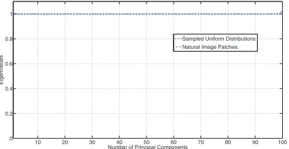
To exemplify Remark IV, we applied IGO-PCA to 100 natural image patches (please see Section 3 of our sup-plementary material for the implementation details of IGO-PCA). Since we have seen that such images are very likely to be pixel-wise dissimilar according to Definition I, we expect that zHi zj 0,∀i, j which further implies
Q = Q2. Then according to Remark IV, the obtained
eigen-spectrum should be approximately equal to the identity matrix. In a similar setting (using IGO-PCA), we computed the eigen-spectrum of samples drawn from Matlab’s random number generator. Fig. 4 plots the two eigen-spectrums.
10 20 30 40 50 60 70 80 90 100 0
0.2 0.4 0.6 0.8 1
Number of Principal Components
Eigenvalues
Sampled Uniform Distributions Natural Image Patches
Fig. 4. The eigen-spectrum of natural images and the eigen-spectrum of samples drawn from Matlab’s random number generator.
3.3 Connection to robust PCA
In this section, we show how the proposed method is related to previously proposed robust extensions to PCA. Such extensions have been the focus of research in statistics [28], [29] and computer vision [23], [30], [31], [32], [33] for several decades. Here, we focus on the general M-Estimation framework of [23] where the problem is posed as the minimization of a robust en-ergy function. This minimization is reformulated as a weighted least-squares problem which can be solved using iteratively re-weighted least-squares. For complex
data, this weighted least-squares energy function has the following form
(U,C,W) =
n
i=1
(zi−Uci)HWi (zi−Uci)
= n
i=1 zH
i Wizi −2zHi Wi Uci
+ cH
i UHWi Uci (12)
where U are the projection bases, ci ∈ CK is the K−dimensional embedding of zi and Wi ∈ RN(P)×N(P)=diag(wi )is the diagonal matrix
contain-ing the weightcontain-ing coefficients used to down-weigh the outliers in zi. Note that
• The embedding ci is not obtained from a least-squares projection, i.e.ci =UHzi.
• AllU,ci,Wi are unknown and have to be estimated from the data.
• The minimization is performed iteratively (using it-erative least-squares) and results in a local minimum of the energy function in (12).
• At each iteration, we updateci from
cnew
i = ((Uold)HWoldi Uold)−1(Uold)HWoldi zi. (13)
To show how robust weighted least-squares is related to our method, we first assume that the projection bases can be written as a linear combination of the data, i.e.
U = ZA for problem (12) and similarly U = ZA for problem (9). Note that this assumption is always true for Small Size Problems (i.e.N(P)n) which is the typical case in subspace learning for appearance-based object recognition. Based on this assumption, we can write
(U,C,W) =
n
i=1 zH
i Wizi−2ziHWiZAci
+ cH
i AHZHWiZAci, (14)
while at each iterationci is updated from
cnew
i = ((Aold)HZHWioldZAold)−1(Aold)HZWoldi zi. (15)
Let us now consider the cost function of IGO-PCA in (9). By plugging C = UHZ and U = ZA into (9) and then expanding, we have
(U,C) =
n
i=1 zH
i zi−2zHi Uci+cHi UHUci
=
n
i=1 zH
i zi−2zHi ZAci+cHi AHZHZAci,
(16)
where we can also write
ci = UHzi =IAHUHzi
[image:5.612.72.281.426.534.2]A simple comparison between (14) and (16) as well as (15) and (17) shows that the main difference is the inclusion of the weights Wi in (14) and (15). We now outline the main result of this section
In IGO-PCA, the weights used to down-weigh the effects of outliers are calculated implicitly.
More specifically, for any of the inner products, if Remark I and II hold, then we can write
zH
i zj =zHi Wijzj (18)
where Wij =diag(wij)is a diagonal matrix containing weights according to
wij(k) =
1 if k∈ P1
if k∈ P2 (19)
where →0 and Wii =I. UsingWij and the fact that
ZHZ= [zH
l zk] = [zHl Wlkzk](16) can be written as
(U,C) =
n
i=1 zH
i Wiizi
− 2[zH
i Wi1z1. . .ziHWinzn]Aci (20)
+ cH
i AH[zHl Wlkzk]Aci
Similarly to standard weighted least-squares, Wij is used to down-weigh the effect of outliers in eitherzi or
zj or both. Note however that Wij is never calculated explicitly by our algorithm and is simply a direct by-product of our analysis in the previous subsections.
A second difference is that there is no fixed Wi for each zi, but weighting matrices Wij corresponding to pairs (zi, zj). We believe that this difference results in a more natural way for defining the notion of outliers at least for computer vision applications. Consider for example the problem of subspace learning for face recog-nition where one or more subjects wear glasses. In this case, it is unclear if glasses should be considered as a part of the appearance or not. In the weighted least-squares of [23], the algorithm would attempt to down-weigh the effect of glasses by assigning small valueswi(kglasses)for
all subjects wearing glasses for the corresponding pixel locations kglasses. However, it is unclear whether this is
correct or not when, for example, 50%of the subjects in the database wear glasses. On the other hand, the notion of outliers in our algorithm is defined more naturally in a bilateral way. If one of zi and zj wears glasses, then
wij(kglasses) =. Note that if bothzi andzj wear glasses,
then wij(kglasses) = 1.
Finally, compared to weighted least-squares, the pro-posed IGO-PCA is non-iterative, requires the eigen-decomposition of a covariance matrix and results in a global optimum solution.
4
E
VALUATION OF ROBUSTNESS OFIGO-PCA
4.1 Face reconstruction
The estimation of a low-dimensional subspace from a set of a highly-correlated images is a typical application of PCA [34]. As an example, we considered a set of 50 aligned face images of image resolution192×168taken from the Yale B face database [35]. The images capture the face of the same subject under different lighting conditions. This setting usually induces cast shadows as well as other specularities. Face reconstruction from the principal subspace is a natural candidate for removing these artifacts.
We initially considered two versions of this experi-ment. The first version used the set of original images. In the second version, 20% of the images was artifi-cially occluded by a 70 ×70 “Baboon” patch placed at random spatial locations. For both experiments, we reconstructed pixel intensities and gradient orientations with standard PCA and IGO-PCA respectively, using the first 5 principal components (please see Section IV of the supplementary material for the implementation details of IGO-PCA).
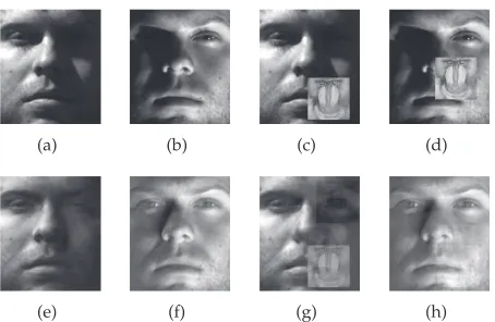
Fig. 5 and Fig. 6 illustrate the quality of reconstruc-tion for 2 examples of face images considered in our experiments. While PCA-based reconstruction of pixel intensities is visually appealing in the first experiment, Fig. 5 (g)-(h) clearly illustrate that, in the second exper-iment, the reconstruction results suffer from artifacts. In contrary, Fig. 6 (e)-(f) and (g)-(h) show that IGO-PCA not only reduces the effect of specularities but also reconstructs the gradient orientations corresponding to the “face” component only.
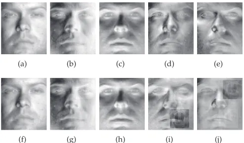
This performance improvement becomes more evident by plotting the principal components for each method and experiment. Fig. 7 shows the 5 dominant Eigenfaces of PCA on image intensities. Observe that, in the second experiment, the last two Eigenfaces (Fig. 7 (i) and (j)) contain “Baboon” ghosts which largely affect the quality of reconstruction. On the contrary, a simple visual in-spection of Fig. 8 reveals that, in the second experiment, the principal subspace of gradient orientations (Fig. 8 (f)-(j)) appears to be artifact-free which in turn makes dis-occlusion in the orientation domain feasible.
Finally, to exemplify Remark III (from section 3.2), we considered a third version of our experiment where 20% of the images were replaced bythe same 192×168
“Baboon” image. Fig. 9 (a)-(e) and (f)-(j) illustrate the principal subspace of pixel intensities and gradient ori-entations respectively. Clearly, we can see that 2 PCA
experiment.
4.1.1 Quantitative evaluation
We used the second version of the above experiment (i.e., 20% of the images were artificially occluded by a “Baboon” patch placed at random spatial locations) to evaluate the robust performance of IGO-PCA quantita-tively and compare it with that of previously proposed robust versions of PCA, namely theR1-PCA [36], the1
-PCA[31], the very recently proposed HQ-PCA [37], the state-of-the-art R-PCA? of [33] as well as the standard
2-PCA. Because these methods operate in the intensity
domain, while IGO-PCA operates in the gradient orien-tation domain, we used a performance measure which does not depend on the specific domain. More specifi-cally, for each of these methods, we computed a measure of total similarity between the principal subspace for the noise-free case Unoise-free and the principal subspace for the noisy caseUnoisy as follows
Q=
k
i=1 k
j=1
cosαij, (21)
where αij is the angle between each of the k
eigen-vectors defining the principal components of Unoise-free and each one of Unoisy [38] 4. The value of Q lies betweenk(coincident spaces) and 0 (orthogonal spaces) [38]. Fig. 10 shows the mean values of Q obtained for each method over 20 repetitions of the experiment for generatingUnoisy. As we may observe, IGO-PCA largely outperforms R1-PCA, 1-PCA, HQ-PCA as well as 2
-PCA while up to k = 5 components the difference from the ideal case (i.e.Unoise-free =Unoisy) is essentially negligible.
Additionally, the performance of IGO-PCA is compa-rable to that of the recent breakthrough of [33]. At this point, we note that
• IGO-PCA is as efficient as standard 2 norm PCA
and thus orders of magnitude faster than [33] (for example for the proposed method needs 0.05secs in a machine running i7 1.7GHz with 8GB Ram and Matlab 64 while the exact method by Candes et. al. 16secs ).
• In contrast to [33], IGO-PCA enables the straightfor-ward embedding of new samples. This is necessary for many computer vision applications such as face recognition and tracking.
• In contrast to [33], our IGO-PCA can be imple-mented incrementally. Please see section 7 of our paper where we propose an efficient and exact online version of our IGO-PCA and show how this algorithm can boost the performance of appearance-based tracking.
4. Note that Q is meaningful as a measure of robustness only if the eigenvectors are orthogonal to each other. Therefore, in our experiments, we have not considered the robust PCA of [23].
(a) (b) (c) (d)
[image:7.612.325.552.54.202.2](e) (f) (g) (h)
Fig. 5. PCA-based reconstruction of pixel intensities. (a)-(b) Original images used in version 1 of our experiment. (c)-(d) Corrupted images used in version 2 of our ex-periment. (e)-(f) Reconstruction of (a)-(b) with 5 principal components. (g)-(h) Reconstruction of (c)-(d) with 5 prin-cipal components.
(a) (b) (c) (d)
(e) (f) (g) (h)
Fig. 6. PCA-based reconstruction of gradient orienta-tions. (a)-(b) Original orientations used in version 1 of our experiment. (c)-(d) Corrupted orientations used in version 2 of our experiment. (e)-(f) Reconstruction of (a)-(b) with 5 principal components. (g)-(h) Reconstruction of (c)-(d) with 5 principal components.
4.2 Face recognition
PCA-based feature extraction for face recognition goes back to the classical work of eigenfaces [20] and still re-mains a standard benchmark for performance evaluation of new algorithms. We considered a single-sample-per-class experiment using aligned frontal-view neutral face images taken from the AR database [39]. Our training test consisted of 100 face images of 100 different subjects, taken fromsession 1. Our testing set consisted of 1 image per subject taken fromsession 2.
4.2.1 Robustness to occlusion
[image:7.612.324.552.297.445.2](a) (b) (c) (d) (e)
[image:8.612.51.298.56.201.2](f) (g) (h) (i) (j)
Fig. 7. The 5 principal components of pixel intensities for (a)-(e) version 1 and (f)-(j) version 2 of our experiment.
(a) (b) (c) (d) (e)
[image:8.612.315.563.56.204.2](f) (g) (h) (i) (j)
Fig. 8. The 5 principal components of gradient orien-tations for (a)-(e) version 1 and (f)-(j) version 2 of our experiment.
features) achieved by IGO-PCA as a function of the percentage of occlusion. The same figure also shows the performance of complex Gabor features combined with PCA, Gabor-Magnitude features combined with PCA, and histograms of Local Binary Patterns (LBP) of cell size 8×8and16×16(please see our experimental section for more details on how these methods were implemented). As we may observe, our method features by far the most robust performance with a recognition rate over 80% even when the percentage of occlusion is about75%. LBP features also perform well, but as further experiments have shown, this performance significantly drops for the case of real occlusions (please see experiment 3 of section 6.4).
4.2.2 Robustness to misalignment
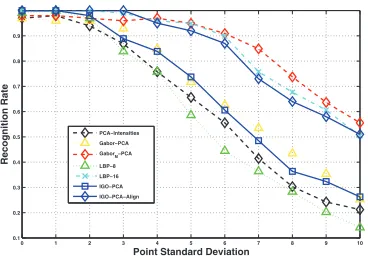
We evaluated the effect of misalignment on the per-formance of our algorithm. Each misaligned test image was artificially generated as follows. We initially selected three fixed canonical points and perturbed these points using Gaussian noise of standard deviation σ. Using the affine warp that the original and perturbed points defined, we generated the affine distorted image. Fig. 12 shows the best recognition rate (over 100 features
(a) (b) (c) (d) (e)
(f) (g) (h) (i) (j)
Fig. 9. (a)-(e) The 5 principal components of pixel in-tensities for version 3 of our experiment and (f)-(j) The 5 principal components of gradient orientations for the same experiment.
1 2 3 4 5 6 7 8 9
1 2 3 4 5 6 7 8 9
Q
Number of Components k
IDEAL
PCA
R1−PCA
L1−PCA
R−PCA?
IGO−PCA
HQ−PCA
Fig. 10. The mean values of the measure of robustness Qas a function of the number of principal componentsk.
0 0.1 0.2 0.3 0.4 0.5 0.6 0.7 0.8 0.9 1 0
0.1 0.2 0.3 0.4 0.5 0.6 0.7 0.8 0.9 1
Recognition Rate
Percentage of Occlusion
PCA−Intensities Gabor−PCA Gabor
M−PCA
LBP−8 LBP−16 IGO−PCA
Fig. 11. Recognition rate as a function of the percentage of occlusion.
[image:8.612.52.298.251.395.2] [image:8.612.359.517.280.413.2] [image:8.612.347.527.466.608.2]robust performance is achieved by Gabor-Magnitudes and16×16LBPs. We found however that these features performed notably well only on the specific experiment. For example, Gabor-Magnitudes do not perform well for the case of illumination (please see section 6.1) or occlusion (sections 4.2.1 and 6.4). Additionally,8×8LBPs largely outperform the 16×16 implementation for case of illumination changes (section 6.1) and real occlusions (section 6.4).
Finally, it is unclear how to use Gabor-Magnitudes or LBP features (or any kind of invariant features) for per-forming joint alignment and recognition as for example in [40], [41]. In contrast, this is feasible with IGO-PCA. For instance, here, we have considered a combination of IGO-PCA with the alignment framework of [40] which we coin IGO-PCA-Align. Fig. 12 shows the performance improvement using IGO-PCA-Align. We may observe that for moderate misalignment (σ = 5), the
improve-ment over IGO-PCA is more than15%.
0 1 2 3 4 5 6 7 8 9 10
0.1 0.2 0.3 0.4 0.5 0.6 0.7 0.8 0.9 1
Recognition Rate
Point Standard Deviation PCA−Intensities
Gabor−PCA
GaborM−PCA
LBP−8 LBP−16
IGO−PCA
[image:9.612.84.268.295.424.2]IGO−PCA−Align
Fig. 12. Recognition rate as a function of the point standard deviation.
5
D
ISCRIMINANT AND MANIFOLD LEARNING FROM IMAGE GRADIENT ORIENTATIONSDiscriminant and manifold subspace analysis is a natural extension to PCA for appearance-based object recogni-tion. Perhaps, the most popular and well-established discriminant and manifold learning methods include Fisher’s Linear Discriminant Analysis (LDA) [21], Lo-cally Linear Embedding (LLE) [1] and Laplacian Eigen-maps (LE) [3]. In this section, we show how to formulate the IGO-versions of these methods.
To do so in a principled way, we need the following theorem (please, see Section II of supplementary material for a proof).
Theorem II. Let A ∈ Cr×r and B ∈ Cr×r be two
Hermitian positive definite matrices. Then, the optimal solution Uo to the following optimization problem
Uo = arg min(max)U∈Cr×Ktr UHAU
s.t. UHBU=I. (22)
is given by the K eigenvectors ofB−1A corresponding to the K smallest (largest) eigenvalues.
Based onTheorem II, the derivation of many popular subspace learning techniques within our framework of image gradient orientations becomes straightforward. As a first example, note that IGO-PCA solves (22) withA=
ZZH and B=I.
As a second example, we describe how to formulate LDA. Let us assume that our training set consists of C
classesC1,· · · ,CC. LDA aims at finding discriminant
pro-jection bases by exploiting this class-label information [21], [18]. Let us also define the complex within-class scatter matrixSzw
Sz w
C
c=1
zi∈Cc
(zi−mc)(zi−mc)H, (23)
where mc = N1(C)Nzi∈Cczi and the complex between-class scatter matrix Szb
Sz b
C
c=1
N(Cc)(mc−m)(mc−m)H. (24)
Then, to find K optimal projections U = [u1|. . .|uk] ∈
CN(P)×K, we solve the following optimization problem Uo = arg maxUtr UHSzbU
s.t. UHSzwU=I (25)
According to (22), the solution is given by theK eigen-vectors of (Szw)−1Szb corresponding to the K largest eigenvalues. Finally, in a similar fashion, we derive the IGO-versions of LLE and LE as well as a number of extensions in Sections III and IV of the supplementary material of this paper.
6
F
ACE RECOGNITION EXPERIMENTSWe evaluated the performance of the proposed IGO-methods for the application of face recognition, per-haps the most representative example of appearance-based object recognition. For our experiments we used the widely used Extended Yale B [35], [42], PIE [43], FERET [44], [45] and AR databases [39]. Our experiments span a wide range of facial variability and moderately controlled capturing conditions: facial expressions (PIE, AR and FERET), illumination changes (Yale B, PIE, AR and FERET), occlusions (AR), aging (FERET) and slight changes in pose (PIE and FERET). We performed experi-ments using a single sample per class (AR and FERET) as well as more than one samples per class (Extended Yale B, PIE and AR). For all experiments, we used manually aligned cropped images of resolution64×64.
In all experiments, we encountered Small Sample Size (SSS) problems (i.e. n N(P)). This setting inevitably
[21]. Finally, given a test vector z, we extracted features using c = UHz and performed classification using the nearest-neighbor rule based on normalized correlation [46], [47], [14]. More details on the implementation of IGO-Methods can be found in Section IV of the accom-panying supplementary material.
We also compared the performance of IGO-methods with that of subspace methods based on pixel intensities and Gabor features as well as with that of LBP methods. For Gabor features, we used the popular approach of [5], [46], [47]. In particular, we used a filter bank of 5 scales and 8 orientations and then down-sampled the obtained features by a factor of 4 (so that the number of features is reasonably large). We considered both phase and magnitude (denoted as Gabor) as well as magnitude information solely (denoted as GaborM). We also produced standard (of radius 2 with 8-samples) uniform LBP descriptors using the MATLAB source code available from [48], [49]. We considered cells of size8×8 (denoted as LBP-8) and 16×16 (denoted as LBP-16). Finally, we found that LBP methods did not perform well for image size 64×64; therefore, for all experiments, we used images of resolution 128×128.
Our methods performed the best in three important as-pects. First, with the exception of the expression experi-ment on AR database, they achieved the best recognition performance in all experiments. The gain in recognition accuracy (in absolute terms) is approximately up to 18% for Yale B, 8% for PIE, 25% for FERET and 20% for AR. Second, there is no other method which performed better than any of the proposed IGO-methods. Even with IGO-PCA, we obtained performance improvement which goes up to 20%. Third, there is no other method which performed the second best consistently. In some experiments, Gabor features outperform LBP features and vice versa.
Finally, to evaluate the statistical significance of our results, we used the McNemars test [50]. McNemars test is a null hypothesis statistical test based on a Bernoulli model. If the resulting p-value is below a desired sig-nificance level (for example, 0.02), the null hypothesis is rejected and the difference in performance between two algorithms is considered to be statistically significant. The McNemars test has been widely used to evaluate the statistical significance of the performance improve-ment between different recognition algorithms [51], [6]. With the exception of experiments 1 (expression) and 2 (illumination) on AR database, for all experiments, we found that p0.02. Thus, we conclude that the
perfor-mance improvement obtained using the IGO-methods is statistically significant.
6.1 Extended Yale B database
The extended Yale B database [52] contains 16128 images of 38 subjects under 9 poses and 64 illumination condi-tions. We used a subset which consists of 64 near frontal images for each subject. For training, we randomly se-lected a subset with 5 images per subject. For testing,
we used the remaining images. Finally, we performed 20 different random realizations of the training/test sets. Table 1 and Fig. 4 of supplementary material show the obtained results. As we may observe, the IGO-methods outperform the second best method (8×8LBPs) in terms of recognition accuracy (in absolute terms) for approxi-mately up to 18%. Additionally, Fig. 5 of supplementary material summarizes the results of manifold embedding IGO methods.
6.2 PIE database
The CMU PIE database [43] consists of more than 41,000 face images of 68 subjects. The database contains faces under varying pose, illumination, and expression. We used the five near frontal poses (C05, C07, C09, C27, C29) and a total of 170 images for each subject. For training, we randomly selected a subset with 5 images per sub-ject. For testing, we used the remaining images. Finally, we performed 20 different random realizations of the training/test sets. Table 2 and Fig. 6 of supplementary material summarize our results. As we can see, the IGO-methods outperform the second best method (Gabor-Magnitude PCA) in terms of recognition accuracy (in absolute terms) for approximately up to 8%. Finally, Fig. 7 of supplementary material summarizes the results of manifold embedding IGO methods.
6.3 FERET database
We carried out single-sample-per-class face recognition experiments on the FERET database [44], [45]. The eval-uation methodology requires that the training must be performed using the FA set which contains one frontal view per subject and in total 1196 subjects. No other data set was used for training. The testing sets include the FB, DupI and DupII data sets. Since current techniques achieve almost 100% recognition performance on FB, we used only Dup I and II in our experiments. DupI and DupII probe sets contain 727 and 234 test images, respectively, captured significantly later than FA. These data sets are very challenging due to significant appear-ance changes of the individual subjects caused by aging, facial expressions, glasses, hair, moustache, non-uniform illumination variations and slight changes in pose.
Table 3 summarizes our results. Previously published results are summarized in Table III of supplementary material. The proposed IGO-PCA achieved recognition rates equal to 89.1% and 85.3% for DupI and DupII respectively which are among the best reported results according to the best of our knowledge.
6.4 AR database
IGO Methods Intensity Methods Gabor Methods LBP Methods IGO-PCA IGO-LDA Intens-PCA Intens-LDA Gabor-PCA Gabor-LDA GaborM-PCA GaborM-LDA LBP-8 LBP-16 95.65%(188) 97.80%(37) 76.10%(161) 72.23%(37) 73.90%(74) 64.38%(12) 64.57%(174) 68.86%(22) 80.00% 60.35%
TABLE 1
Average recognition rates on the extended Yale B database. In parentheses the dimension that results in the best performance for each method is given.
IGO Methods Intensity Methods Gabor Methods LBP Methods
IGO-PCA IGO-LDA Intens-PCA Intens-LDA Gabor-PCA Gabor-LDA GaborM-PCA GaborM-LDA LBP-8 LBP-16 84.56%(335) 88.36%(50) 32.35%(339) 77.53%(67) 68.75%(136) 67.19%(31) 72.17%(296) 80.35%(51) 68.60% 65.00%
TABLE 2
Average recognition rates on the PIE database. In parentheses the dimension that results in the best performance for each method is given.
Methods Intens-PCA LBP-8 LBP-16 Gabor-PCA GaborM-PCA IGO-PCA
DupI 45% 65% 58% 60% 57% 88.9%
[image:11.612.155.461.228.268.2]DupII 29% 62% 53% 55% 50% 85.4%
TABLE 3
Recognition rates for DupI and DupII.
IGO Methods Intensity Methods Gabor Methods LBP Methods
[image:11.612.47.568.310.368.2]IGO-PCA IGO-LDA Intens-PCA Intens-LDA Gabor-PCA Gabor-LDA GaborM-PCA GaborM-LDA LBP-8 LBP-16 Exper. 1 97.33%(131) 97.67%(99) 91.67%(169) 94.33%(99) 96.67%(101) 89.33%(70) 98.00%(170) 98.67%(96) 89.67% 95.33% Exper. 2 100.00%(30) 99.67%(30) 94.67%(358) 92.67%(99) 97.67%(145) 96.67%(99) 97.00%(307) 96.77%(99) 99.00% 98.67% Exper. 3 94.50%(99) 95.20%(99) 37.72%(344) 45.58%(99) 28.33%(178) 30.00%(68) 40.00%(322) 47.66%(94) 73.33% 60.66%
TABLE 4
Recognition rates on the AR database for facial expressions (experiment 1), illumination variations (experiment 2), and occlusions-illumination changes (experiment 3). In parentheses the dimension that results in the best
performance for each method is given.
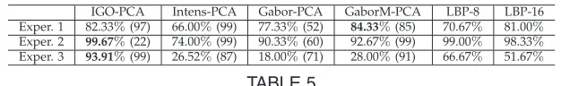
[image:11.612.149.462.424.472.2]IGO-PCA Intens-PCA Gabor-PCA GaborM-PCA LBP-8 LBP-16 Exper. 1 82.33%(97) 66.00%(99) 77.33%(52) 84.33%(85) 70.67% 81.00% Exper. 2 99.67%(22) 74.00%(99) 90.33%(60) 92.67%(99) 99.00% 98.33% Exper. 3 93.91%(99) 26.52%(87) 18.00%(71) 28.00%(91) 66.67% 51.67%
TABLE 5
Recognition rates for the single-sample-per-class experiment on the extended AR database facial expressions (experiment 1), illumination variations (experiment 2), and occlusions-illumination changes (experiment 3). In
parentheses the dimension that results in the best performance for each method is given.
different facial expressions (1-4), illumination changes (5-7), and different occlusions under different illumination changes (8-13). The second session duplicates the first session two weeks later. We randomly selected a subset with 100 subjects. Fig. 13 shows a sample of images used in our experiments. We investigated the robustness of our scheme for the case of facial expressions (ex-periment 1), illumination variations (ex(ex-periment 2), and occlusions-illumination changes (experiment 3). More specifically, we carried out the following experiments.
[image:11.612.385.489.543.613.2]1) In experiment 1, we used images 1-4 of session 1 for training and images 2-4 of session 2 for testing. 2) In experiment 2, we used images 1-4 of session 1 for training and images 5-7 of session 2 for testing. 3) In experiment 3, we used images 1-4 of session 1 for training and images 8-13 of session 2 for testing.
Fig. 13. Face images of the same subject taken from the AR database.
database, IGO-methods largely outperformed all other methods. More specifically the gain in recognition accu-racy goes up to 20%. In contrast to experiments 1 and 2, these results are statistically significant. Additionally, Fig. 9 of supplementary material summarizes the results of manifold embedding IGO methods.
Furthermore, Table 5 and Fig. 10 of supplementary material summarize the results for our single sample per class experiments. For this setting, we used only image 1 of session 1 for training. As our results show, IGO-PCA achieves almost 100% recognition rate for the case of illumination changes (experiment 2) and approximately 94% recognition rate for the case of occlusions (exper-iment 3). The latter result is approximately 20% better than the best reported recognition rate [53], which was obtained on a subset of the occluded images with no illumination variations and more than 25% better than the rate achieved by 8×8 LBP. Finally, for the case of facial expressions (experiment 1) Gabor-Magnitude PCA performs better than IGO-PCA. A further analysis of this result has shown that all of the misclassified face images were faces having the expression of scream. This result is somewhat expected, since, as Fig. 13 (c) illustrates, screaming results in severe non-rigid facial deformations which, in turn, cause significant local orientation mis-matches. These mismatches inevitably render the values of within and between-class similarity comparable.
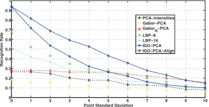
Finally, we carried out perhaps one of the most dif-ficult experiments in face recognition: single sample per class recognition of misaligned frontal faces with occlusions and illumination changes in the testing set. More specifically, our experimental setting combined the single sample per class experiment 3 on AR database with the misalignment experiment of Section 4.2.2. Fig. 14 shows the recognition rates achieved by all methods as a function of misalignment. We may observe that the proposed methods and especially IGO-PCA-Align largely outperform all other methods.
0 1 2 3 4 5 6 7 8 9 10
0 0.1 0.2 0.3 0.4 0.5 0.6 0.7 0.8 0.9 1
Recognition Rate
Point Standard Deviation
[image:12.612.70.280.530.638.2]PCA−Intensities Gabor−PCA GaborM−PCA LBP−8 LBP−16 IGO−PCA IGO−PCA−Align
Fig. 14. Recognition rate as a function of the point standard deviation.
7
A
PPLICATION TO TRACKINGSubspace learning for appearance-based tracking has been one of the de facto choices for tracking objects in image sequences [54], [55], [56]. Here, we propose a
subspace-based tracking algorithm closely related to the incremental visual tracker of [56]. As such, our tracker can deal with drastic appearance changes, does not require offline training, continually updates a compact object representation and uses the Condensation algo-rithm to robustly estimate the object’s location.
Similarly to [56], the proposed tracker is essentially an eigen-tracker [54], where the eigen-space is adap-tively learned and updated online. The key element which makes our approach equally fast but significantly more robust, is how the eigen-space is generated. The method in [56] uses the incremental version of stan-dard intensity-based PCA [57]. On the contrary, the proposed tracker is based on the eigenspace gener-ated by IGO-PCA. Let us assume that, given n images
{I1, . . . ,In}, we have already computed the principal
subspace Unp and Σnp =Λ1/2p . Then, given a new image
set {In+1, . . . ,In+m}, our target is to obtain Un+m and
Σn+m
p corresponding to{I1, . . . ,In+m}efficiently.
Algo-rithm 3 of our supplementary material summarizes the steps of incremental IGO-PCA. Finally, similarly to [56], the proposed tracker combines our incremental IGO-PCA with a variant of the Condensation algorithm for the dynamical estimation of the object’s location.
We evaluated the performance of the proposed tracker on two very popular video sequences, “Dudek” and “Trellis”, available from http://www.cs.toronto.edu/dross/ivt/. The goal was to assess the proposed algorithm’s performance for face tracking under pose variation, occlusions and non-uniform illumination. “Dudek” is provided along with seven annotated points which are used as ground truth. We also annotated seven fiducial points for “Trellis”. As usual, quantitative performance evaluation is based on the RMS errors between the true and the estimated locations of these seven points. The performance of our tracker is compared with that of [56]. No attempt to optimize the performance of our method was attempted. For both methods, we used the same particle filter parameters (taken from [56]).
For both methods and sequences, Fig. 12 of supple-mentary material plots the RMS error as a function of the frame number, while Table 6 gives the mean and median RMS error. The proposed tracker outperforms the method of [56] in two important aspects. First, it is more robust. Only the proposed tracker successfully tracked the face for the whole video sequence for both “Dudek” and “Trellis”. Second, the proposed scheme is more accurate. This is illustrated by the RMS error com-puted for frames where the face region was successfully tracked. Finally, Fig. 13 of supplementary material illus-trates the performance of the proposed tracker, as well as the performance of IVT tracker, for some cumbersome tracking conditions.
8
C
ONCLUSIONSorienta-IGO-PCA Intensity-based PCA “Dudek” 6.79 (5.70) 8.24 (7.28)
“Trellis” 2.59 (2.42) 3.83 (3.73)
TABLE 6
Mean (Median) RMS error for “Dudek” and “Trellis” sequences.
tions. Our IGO-based learning framework is as simple as standard intensity-based learning, yet much more pow-erful for efficient subspace-based data representation. Central to the proposed methodology is the distribution of gradient orientation differences and the cosine kernel which provide us a powerful and consistent way to measure image correlation/similarity. We showed that this measure can be naturally used to provide the basis for robust subspace learning. We demonstrated some of the favorable properties of IGO subspace learning for the application of face recognition and tracking.
R
EFERENCES[1] S.T. Roweis and L.K. Saul, “Nonlinear dimensionality reduction by locally linear embedding,”Science, vol. 290, no. 5500, pp. 2323, 2000.
[2] M. Balasubramanian, E.L. Schwartz, J.B. Tenenbaum, V. de Silva, and J.C. Langford, “The isomap algorithm and topological stability,”Science, vol. 295, no. 5552, pp. 7, 2002.
[3] M. Belkin and P. Niyogi, “Laplacian eigenmaps for dimensionality reduction and data representation,” Neural computation, vol. 15, no. 6, pp. 1373–1396, 2003.
[4] L.K. Saul and S.T. Roweis, “Think globally, fit locally: unsu-pervised learning of low dimensional manifolds,” The Journal of
Machine Learning Research, vol. 4, pp. 119–155, 2003.
[5] L. Chengjun, “Gabor-based kernel PCA with fractional power polynomial models for face recognition,” IEEE Transactions on
Pattern Analysis and Machine Intelligence, vol. 26, no. 5, pp. 572 –
581, May 2004.
[6] J. Yang, A.F. Frangi, J. Yang, D. Zhang, and Z. Jin, “KPCA plus LDA: A complete kernel Fisher discriminant framework for feature extraction and recognition,” IEEE Transactions on Pattern
Analysis and Machine Intelligence, vol. 27, no. 2, pp. 230–244, 2005.
[7] X. He, S. Yan, Y. Hu, P. Niyogi, and H.J. Zhang, “Face recognition using laplacianfaces,” IEEE Transactions on Pattern Analysis and
Machine Intelligence, pp. 328–340, 2005.
[8] H. Cevikalp, M. Neamtu, M. Wilkes, and A. Barkana, “Discrimi-native common vectors for face recognition,”IEEE Transactions on
Pattern Analysis and Machine Intelligence, vol. 27, no. 1, pp. 4–13,
2005.
[9] M. Zhu and A.M. Martinez, “Subclass discriminant analysis,”
IEEE Transactions on Pattern Analysis and Machine Intelligence, pp.
1274–1286, 2006.
[10] L. Chengjun, “Capitalize on dimensionality increasing techniques for improving face recognition grand challenge performance,”
IEEE Transactions on Pattern Analysis and Machine Intelligence, vol.
28, no. 5, pp. 725–737, 2006.
[11] D. Cai, X. He, J. Han, and H. Zhang, “Orthogonal laplacianfaces for face recognition,” IEEE transactions on image processing, vol. 15, no. 11, pp. 3608, 2006.
[12] E. Kokiopoulou and Y. Saad, “Orthogonal neighborhood pre-serving projections: A projection-based dimensionality reduction technique,” IEEE Transactions on Pattern Analysis and Machine
Intelligence, vol. 29, no. 12, pp. 2143, 2007.
[13] G. Goudelis, S. Zafeiriou, A. Tefas, and I. Pitas, “Class-Specific Kernel-Discriminant Analysis for Face Verification,” IEEE
Trans-actions on Information Forensics and Security, vol. 2, no. 3 Part 2,
pp. 570–587, 2007.
[14] X. Jiang, B. Mandal, and A. Kot, “Eigenfeature regularization and extraction in face recognition,” IEEE Transactions on Pattern
Analysis and Machine Intelligence, vol. 30, no. 3, pp. 383–394, 2008.
[15] J. Wright, A. Yang, A. Ganesh, S. Sastry, and Y. Ma, “Robust face recognition via sparse representation,” IEEE Transactions on
Pattern Analysis and Machine Intelligence, vol. 31, no. 2, pp. 210–227,
2009.
[16] G. Baudat and F. Anouar, “Generalized discriminant analysis using a kernel approach,”Neural Comput., vol. 12, pp. 2385–2404, 2000.
[17] H. Cevikalp, M. Neamtu, and M. Wilkes, “Discriminative com-mon vector method with kernels,” IEEE Transactions on Neural
Networks, vol. 17, no. 6, 2006.
[18] H. Li, T. Jiang, and K. Zhang, “Efficient and robust feature extraction by maximum margin criterion,” IEEE Transactions on
Neural Networks, vol. 17, no. 1, pp. 157–165, Jan. 2006.
[19] X. He, D. Cai, S. Yan, and H.-J. Zhang, “Neighborhood preserving embedding,”Computer Vision, IEEE International Conference on, vol. 2, pp. 1208–1213, 2005.
[20] M. Turk and A. Pentland, “Eigenfaces for recognition,”Journal of
cognitive neuroscience, vol. 3, no. 1, pp. 71–86, 1991.
[21] P. N. Belhumeur, J. P. Hespanha, and D. J. Kriegman, “Eigenfaces vs. Fisherfaces: Recognition using class specific linear projection,”
IEEE Transactions on Pattern Analysis and Machine Intelligences, vol.
19, no. 7, pp. 711–720, 1997.
[22] G. Tzimiropoulos, V. Argyriou, S. Zafeiriou, and T. Stathaki, “Robust FFT-Based Scale-Invariant Image Registration with Image Gradients,” IEEE Transactions on Pattern Analysis and Machine
Intelligence, accepted for publication.
[23] F. De La Torre and M.J. Black, “A framework for robust subspace learning,” International Journal of Computer Vision, vol. 54, no. 1, pp. 117–142, 2003.
[24] H.P. Frey, P. Konig, and W. Einhauser, “The Role of First and Second-Order Stimulus Features for Human Overt Attention,”
Perception and Psychophysics, vol. 69, pp. 153–161, 2007.
[25] A. Papoulis and S.U. Pillai, Probability, random variables, and
stochastic processes, McGraw-Hill New York, 2004.
[26] AJ Fitch, A. Kadyrov, W.J. Christmas, and J. Kittler, “Orientation correlation,” inBritish Machine Vision Conference, 2002, vol. 1, pp. 133–142.
[27] A. Ros, “A two-piece property for compact minimal surfaces in a three-sphere,” Indiana University Mathematics Journal, vol. 44, no. 3, pp. 841–850, 1995.
[28] N.A. Campbell, “Robust procedures in multivariate analysis I: Robust Covariance estimation,” Applied Statistics, vol. 29, no. 3, pp. 231–237, 1980.
[29] C. Croux and G. Haesbroeck, “Principal component analysis based on robust estimators of the covariance or correlation matrix: influence functions and efficiencies,”Biometrika, vol. 87, no. 3, pp. 603, 2000.
[30] Q. Ke and T. Kanade, “Robust L/sub 1/norm factorization in the presence of outliers and missing data by alternative convex programming,” inIEEE Computer Society Conference on Computer
Vision and Pattern Recognition, 2005. CVPR 2005, 2005, vol. 1.
[31] N. Kwak, “Principal component analysis based on L1-norm maximization,” IEEE transactions on pattern analysis and machine
intelligence, vol. 30, no. 9, pp. 1672–1680, 2008.
[32] V. Chandrasekaran, S. Sanghavi, P.A. Parrilo, and A.S. Willsky, “Rank-sparsity incoherence for matrix decomposition,” preprint, 2009.
[33] E.J. Candes, X. Li, Y. Ma, and J. Wright, “Robust principal component analysis?,” Arxiv preprint arXiv:0912.3599, 2009. [34] M. Kirby and L. Sirovich, “Application of the karhunen-loeve
procedure for the characterization of human faces.,” IEEE
Trans-actions Pattern Analysis and Machine Intelligence, vol. 12, no. 1, pp.
103–108, Jan. 1990.
[35] A.S. Georghiades, P.N. Belhumeur, and D.J. Kriegman, “From few to many: Illumination cone models for face recognition under variable lighting and pose,” IEEE Transactions on Pattern Analysis
and Machine Intelligence, vol. 23, no. 6, pp. 643–660, 2001.
[36] C. Ding, D. Zhou, X. He, and H. Zha, “R 1-pca: rotational invari-ant l 1-norm principal component analysis for robust subspace factorization,” inProceedings of the 23rd international conference on
Machine learning. ACM, 2006, pp. 281–288.
[37] R. He, B.-G. Hu, W.-S. Zheng, and X.-W. Kong, “Robust principal component analysis based on maximum correntropy criterion,”
IEEE Transactions on Image Processing, vol. 20, no. 6, pp. 1485 –
[38] WJ Krzanowski, “Between-groups comparison of principal com-ponents,” Journal of the American Statistical Association, pp. 703– 707, 1979.
[39] AM Martinez and R. Benavente, “The AR face database,” Tech. Rep., CVC Technical report, 1998.
[40] S. Yan, H. Wang, J. Liu, X. Tang, and T.S. Huang, “Misalignment-robust face recognition,” Image Processing, IEEE Transactions on, vol. 19, no. 4, pp. 1087–1096, 2010.
[41] A. Wagner, J. Wright, A. Ganesh, Z. Zhou, and Y. Ma, “Towards a practical face recognition system: robust registration and illumi-nation by sparse representation,” inComputer Vision and Pattern
Recognition, 2009. CVPR 2009. IEEE Conference on. Ieee, 2009, pp.
597–604.
[42] K.C. Lee, J. Ho, and D.J. Kriegman, “Acquiring linear subspaces for face recognition under variable lighting,”IEEE Transactions on
Pattern Analysis and Machine Intelligence, pp. 684–698, 2005.
[43] T. Sim, S. Baker, and M. Bsat, “The CMU pose, illumination, and expression database,” IEEE Transactions on Pattern Analysis and
Machine Intelligence, pp. 1615–1618, 2003.
[44] P. J. Phillips, H. Moon, P. J. Rauss, and S. Rizvi, “The FERET evaluation methodology for face recognition algorithms,” IEEE
Transactions on Pattern Analysis and Machine Intelligence, vol. 22,
no. 10, pp. 1090–1104, 2000.
[45] P.J. Phillips, H. Wechsler, J. Huang, and P. Rauss, “The FERET database and evaluation procedure for face recognition algo-rithms,” Image and Vision Computing, vol. 16, no. 5, pp. 295–306, 1998.
[46] L. Chengjun and H. Wechsler, “Gabor feature based classification using the enhanced Fisher linear discriminant model for face recognition,” IEEE Transactions on Image Processing, vol. 11, no. 4, pp. 467 – 476, Apr. 2002.
[47] L. Chengjun and H. Wechsler, “Independent component analysis of gabor features for face recognition,”IEEE Transactions on Neural
Networks, vol. 14, no. 4, pp. 919–928, July 2003.
[48] T. Ahonen, A. Hadid, and M. Pietikainen, “Face description with local binary patterns: Application to face recognition,”IEEE
Transactions on Pattern Analysis and Machine Intelligence, pp. 2037–
2041, 2006.
[49] “http://www.ee.oulu.fi/mvg/page/lbp matlab,” .
[50] Q. McNemar, “Note on the sampling error of the difference between correlated proportions or percentages,” Psychometrika, vol. 12, no. 2, pp. 153–157, 1947.
[51] B.A. Draper, K. Baek, M.S. Bartlett, and J.R. Beveridge, “Rec-ognizing faces with PCA and ICA,” Computer vision and image
understanding, vol. 91, no. 1-2, pp. 115–137, 2003.
[52] K.C. Lee, J. Ho, and D. Kriegman, “Acquiring linear subspaces for face recognition under variable lighting,”IEEE Trans. Pattern
Anal. Mach. Intelligence, vol. 27, no. 5, pp. 684–698, 2005.
[53] H. Jia and A.M. Martinez, “Face recognition with occlusions in the training and testing sets,” inProc. Conf. Automatic Face and
Gesture Recognition. Citeseer, 2008.
[54] M.J. Black and A.D. Jepson, “Eigentracking: Robust matching and tracking of articulated objects using a view-based representation,”
International Journal of Computer Vision, vol. 26, no. 1, pp. 63–84,
1998.
[55] T.F. Cootes, G.J. Edwards, and C.J. Taylor, “Active appearance models,” Pattern Analysis and Machine Intelligence, IEEE
Transac-tions on, vol. 23, no. 6, pp. 681–685, 2001.
[56] D.A. Ross, J. Lim, R.S. Lin, and M.H. Yang, “Incremental learning for robust visual tracking,”International Journal of Computer Vision, vol. 77, no. 1, pp. 125–141, 2008.
[57] A. Levey and M. Lindenbaum, “Sequential karhunen-loeve basis extraction and its application to images,” Image Processing, IEEE
Transactions on, vol. 9, no. 8, pp. 1371–1374, 2000.
Georgios Tzimiropoulosreceived the diploma degree in Electrical and Computer Engineer-ing from Aristotle University of Thessaloniki, Greece, in 2004 and the M.Sc. and Ph.D. de-grees in Signal Processing and Computer Vision both from Imperial College London, U.K., in 2005 and 2009, respectively. He is currently a Lecturer (Assistant Professor) with the School of Com-puter Science at the University of Lincoln, UK. After the completion of his Ph.D., he was working as a Research and Development engineer with Imperial College/Selex Galileo. From 2010 to 2012, he was a Research Associate at the Intelligent Behaviour Understanding Group in the De-partment of Computing at Imperial College working on face analysis. His main research interests are in the areas of face and object recognition, alignment and tracking and facial expression analysis.
Stefanos Zafeiriouis a Research Fellow with Department of Computing, Imperial College London holding one of the prestigious Junior Research Fellowships (JRF) of Imperial College London. He received both B.Sc and PhD de-grees in Informatics with highest honors from the Aristotle University of Thessaloniki, Greece in 2003 and 2007, respectively. He has received various scholarships and awards during his un-dergraduate, Ph.D. and postdoctoral studies. Dr. Zafeiriou is an associate editor of Image and Vision Computing Journal and of IEEE Transactions on Systems, Man, and Cybernetics Part B. He has also served as a program committee member for a number of IEEE international conferences. He has co-authored more than 50 technical papers including more than 20 papers in the most prestigious journals in his field like IEEE Transactions on Pattern Analysis and Machine Intelligence, IEEE Transactions on Image Processing, IEEE Transaction on Visualization and Computer Graphics, IEEE Transactions on Neural Networks, Data Mining and Knowledge Discovery, Pattern Recognition etc.