Removal of Random Valued Impulse Noise with Modified Weighted Mean Filter by using Denoising Algorithm: Emerging Opportunities of Image Processing Application

Removal of Random Valued Impulse Noise with

Modified Weighted Mean Filter by using Denoising

Algorithm: Emerging Opportunities of Image

Processing Application

Nihar Ranjan Hota1, Sitanshu Prativa Pattanaik2, Rajalaxmi Padhy3 1

Assistant Professor, in Dept. of Computer Science & Engineering Einstein Academy of Technology & Management (EATM), Bhubaneswar (India).

2

Research Scholar, Department of CSE, CET, Bhubaneswar 3

Asistant Professor in Dept. of Computer Science & Engineering, CET, Bhubaneswar

Abstract: Digital images play a vital role in image processing which have sundry no of applications in the field of medical science, engineering, space science, agricultural science etc. As a large no of scientific applications are carried out through the help of digital images so it would be quite difficult to get the accurate result if those images are corrupted by noises. Noises are unwanted information in images which arises due to several factors such as inaccurate analog to digital conversion, statistical quantum fluctuation of camera sensors,[1] heat production in sensors and so on. Image noise is random (not present in the object imaged) variation of brightness or color information in images, and is usually an aspect of electronic noise. It can be produced by the sensor and circuitry of a scanner or digital camera. Image noise can also originate in film grain and in the unavoidable short noise of an ideal photon detector. Image noise is an undesirable by-product of image capture that adds spurious and extraneous information. Noise can introduce by transmission errors and compression. So noise reduction is most important task for improve quality of image. Denoising technique is often a necessary and the take first step, before analyzed the image data. It is important apply denoising technique to compensate for such data corruption. Denoising techniques still remains big challenge for researchers because noise removal introduced artifacts and causes blurring of an images. Image Denoising techniques depend on what type of noise occurred in image like Gaussian noise, impulse noise; speckle noise etc. Keywords: Image Processing (IP), Camera Sensor (CS), Quality Of Image (QOI), Blurring Of an Images (BOI), Denoising Techniques (DT)

I. INTRODUCTION

A. Context

Digital images play a vital role in image processing which have sundry no of applications in the field of medical science, engineering, space science, agricultural science etc. As a large no of scientific applications are carried out through the help of digital images so it would be quite difficult to get the accurate result if those images are corrupted by noises.

Noises are unwanted information in images which arises due to several factors such as inaccurate analog to digital conversion, statistical quantum fluctuation of camera sensors,[1] heat production in sensors and so on.

Image noise is random (not present in the object imaged) variation of brightness or color information in images, and is usually an aspect of electronic noise. It can be produced by the sensor and circuitry of a scanner or digital camera. Image noise can also originate in film grain and in the unavoidable short noise of an ideal photon detector

Image noise is an undesirable by-product of image capture that adds spurious and extraneous information. Noise can introduce by transmission errors and compression

So noise reduction is most important task for improve quality of image .Denoising technique is often a necessary and the take first step, before analyzed the image data.

B. Motivation

From the problem statement it can be concluded that removal of SPN is easier rather than RVIN. Most of the reported schemes work well under the SPN but fails under RVIN, which is more realistic when it comes to real world applications. It is also observed the performance of any filtering scheme is dependent on the detection mechanism. The better is the detector; the superior is the filtering performance. Hence the performance of a detector plays a vital role. The detector performance is solely dependent on a threshold value which is compared with a pre computed numerical value. To improve the detector performance need for an adaptive threshold is an utmost necessity which can be automatically determined from the characteristics of an image and the noise present on it.

C. Objective

1) Selection of an image and adding noise in that im

2) To work towards improved and efficient detectors for identifying contaminated pixels and clean pixel. 3) Filtering of noise pixels and replacing them by the filtered pixels.

4) To devise adaptive thresholding techniques so that noise detection would be more reliable

D. Problem Statement

Impulsive noise can be classified as salt-and-pepper noise (SPN) and random-valued impulse Noise (RVIN). An image containing impulsive noise can be described as follows:

x(i, j) = n(i, j)withprobabilityp

y(i, j)withprobability1−p

Where x(i,j)denotes a noisy image pixel, y(i,j) denotes a noise free image pixel and η(i, j) denotes a noisy impulse at the location (i, j). In salt-and-pepper noise, noisy pixels take either minimal or maximal values i.e. n(i,j) € {Lmin,Lmax } and for random-valued impulse noise, noisy pixels take any value within the range minimal to maximal value i.e. n(i,j)€ {Lmin,Lmax } where Lminand Lmax denote the lowest and the highest pixel luminance values within the dynamic range respectively . So that it is little bit difficult to remove random valued impulse noise rather than salt and pepper noise [3]. The main difficulties which have to face for attenuation of noise is the preservation of image details. The difference between SPN and RVIN may be best described by Figure 1.3. In the case of SPN the pixel substitute in the form of noise may be either Lmin(0) or Lmax(255). Where as in RVIN situation it may range from Lmin to Lmax. Cleaning such noise is far more difficult than cleaning fixed-valued impulse noise since for the latter, the differences in gray levels between a noisy pixel and its noise-free neighbors are significant most of the times. In this thesis, we focus only on randomvaluedimpulse noise(RVIN) and schemes are proposed to suppress RVIN.

{0,255} 255 (a)

0 [0,255] 255

(b)

Figure 1: Representation of (a) Salt & Pepper Noise with Ri,j ∈ {nmin, nmax}, (b)Random Valued Impulsive Noise with Ri,j ∈ [nmin, nmax]

E. Thesis Organization

ordered absolute difference to distinguish between a noise or a image details. Implementation and details comparison with median and wiener filter BDND, BRBDNR, NUASM has been made. Chapter 6 represents simulation and experimental results. Chapter leads to a conclusion.

II. IMAGE PROCESSING

A. Introduction

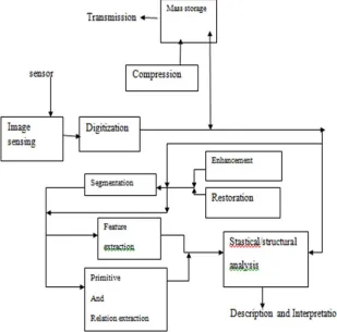
An image may be defined as a two dimensional function, f(x, y), where x and y are spatial coordinates, and the amplitude of f at any pair of coordinates (x, y) is called the intensity or gray level of the image at that point. When x, y and the amplitude values of f are all finite, discrete quantities, then the image can be called as a digital image. The field of digital image processing refers to processing digital images by means of a digital computer. Image restoration is a fundamental step of digital image processing [1]. The entire process of image processing and analysis starting from the receiving of visual information to the giving out description of the scene, may be divided into three major stages which are also considered as major sub-areas, and are given below:

1) Discretization and representation: converting visual information into a discrete form; suitable for computer processing; approximating visual information to save storage space as well as time requirement in subsequent processing.

2) Processing: improving image quality by filtering etc.; compressing data to save storage and channel capacity during transmission.

3) Analysis: extracting image features; quantifying shapes, registration recognition.

In the initial stage, the input is a scene (visual information), and the output is corresponding digital image. In the secondary stage, both the input and the output are images where the output is an improved version of the input. And, in the final stage, the input is still an image but the output is a description of the contents of that image [2].A schematic diagram of different stages is shown in Figure 1.1. The figure is taken from the book specified in [2] Out of the sub-branches of digital image processing, diagrammatically represented below, this thesis deals with image restoration. To be precise, the thesis devotes on a part of the image restoration i.e. noise removal from images. Accurately, it is about the denoising of one particular type of noise i.e. Impulsive noise, stated in the Problem Definition.

B. Image Restoration

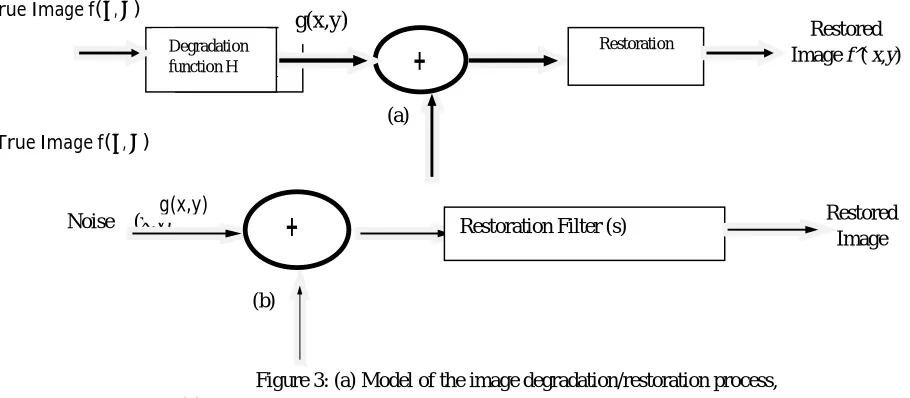
Restoration attempts to reconstruct or recover an image that has been degraded by using a priori knowledge of the degradation phenomenon. Restoration techniques are primarily modeling of the degradation and applying the inverse process in order to recover the original image. The degradation function together with an additive noise operates on an input image f(x, y) to produce a degraded image g(x, y). Given g(x, y), some knowledge about the degradation function h(x, y) and some knowledge about the additive noise term η(x,y) the objective of restoration is to obtain an estimate of the original image [1].

TrueImagef( , )

(a)

TrueImagef( , )

Noise η (x,y)

(b)

Figure 3: (a) Model of the image degradation/restoration process, (b) Model of the Noise Removal Process.

The degraded image is given in spatial domain by g(x, y) = f(x, y) * h(x, y) + η(x, y) (1.1) In this thesis, it is assumed that the degradation function is the identity operator, and it deals only with degradations due to noise. So the degraded image is:

g(x,y) = f(x,y ) + n(x,y) (1)

C. Noise model

Noise is a disturbance that affects a signal and that may distort the information carried by the signal. It can be Random variations of one or more characteristics of any entity such as voltage, current, or data. Otherwise it is a random signal of known statistical properties of amplitude, distribution, and spectral density. Loosely, noise can be defined as any disturbance tending to interfere with the normal operation of a device or system. Image noise is a random, usually unwanted, variation in brightness or color information in an image [23]. Image noise can originate in film grain, or in electronic noise in the input device (scanner or digital camera) sensor and circuitry, or in the unavoidable shot noise of an ideal photon detector. Digital images are prone to a variety of types of noise. Noise is the result of errors in the image acquisition / transmission process that result in pixel values that do not reflect the true intensities of the real scene. There are several ways that noise can be introduced into an image, depending on how the image is created. For example: If the image is scanned from a photograph made on film, the film grain is a source of noise. Noise can also be the result of damage to the film [22], or be introduced by the scanner itself. If the image is acquired directly in a digital format, the mechanism for gathering the data (such as a CCD detector) can introduce noise. Electronic transmission of image data can introduces noise [2]. The spatial component of noise is based on the statistical behavior of the intensity values. These may be considered as random variables, characterized by a probability density function (pdf). A probability density function (pdf), or density, of a random variable is a function which describes the density of probability at each point in the sample space. The probability of a random variable falling within a given set is given by the integral of its density over the set. Some commonly found noises are Gaussian noise, Rayleigh noise, Gamma noise, Exponential noise, Impulsive noise and so on.

D. Different types of noise

Noise in images is caused by the random fluctuations in brightness or color information. Noise represents unwanted information which degrades the image quality. Noise is defined as a process which affects the acquired image quality that is being not a part of the original image content. [44] Digital image noise may occur due to various sources. During acquisition process, digital images convert optical signals into electrical one and then to digital signals and are one process by which the noise is introduced in digital

Degradation Function H Degradatio_{n Function}

Restored Image

+

images. Due to natural phenomena at conversion process each stage experiences a fluctuation that adds a random value to the intensity of a pixel in a resulting image. In general image noise is regarded as an undesirable by-product of image capture. In general image noise is regarded as anundesirable by-product of image capture.The types of Noise are following:-

1) Gaussian noise: Gaussian noise is statistical in nature. Its probability density function equal to that of normal distribution, which is otherwise called as Gaussian distribution. In this type of noise, values of that the noise are being Gaussian-distributed. A special case of Gaussian noise is white Gaussian noise, in which the values always are statistically independent. For application purpose, Gaussian noise is also used as additive white noise to produce additive white Gaussian noise. Gaussian noise is commonly defined as the noise with a Gaussian amplitude distribution, which states that nothing the correlation of the noise in time or the spectral density of noise. Gaussian noise is otherwise said as white noise which describes the correlation of noise. Gaussian noise is sometimes equated to be of white Gaussian noise, but it may not necessarily the case.

2) Salt and pepper noise: In [44], [45], salt & pepper noise model, there is only two possible values ‘a’ and ‘b. The probability of getting each of them is less than 0.1 (else, the noise would greatly dominate the image). For 8 bit/pixel image, the intensity value for pepper noise typically found nearer to 0 and for salt noise it is near to 255. Salt and pepper noise is a generalized form of noise typically seen in images. In image criteria the noise itself represents as randomly occurring white and black pixels. An effective noise reduction algorithm for this type of noise involves the usage of a median filter, morphological filter. Salt and pepper noise occurs in images under situations where quick transients, such as faulty switching take place. This type of noise can be caused by malfunctioning of analog-to-digital converter in cameras, bit errors in transmission, etc.

3) Poisson noise: Poisson noise is also known as [44] shot noise. It is a type of electronic noise. Poisson noise occur under the situations where there is a statistical fluctuations in the measurement caused either due to finite number of particles like electron in an electronic circuit that carry energy, or by the photons in an optical device

E. Speckle Noise

In [44],[46],[47], Speckle noise is a type of granular noise that commonly exists in and causes degradation in the image quality Speckle noise tends to damage the image being acquired from the active radar as well as synthetic aperture radar(SAR) images. Due to random fluctuations in the return signal from an object in conventional radar that is not big as single image-processing element. Speckle noise occurs. Speckle noise increases the mean grey level of a local area. Speckle noise is more serious issue, causing difficulties for image interpretation in SAR images .It is mainly due to coherent processing of backscattered signals from multiple distributed targets.

F. Spatial filtering

Spatial filtering is preferred when only additive noise is present. The different classesof filtering techniques exist in spatial domain filtering.

1) Mean Filter: Mean filtering is a simple, intuitive and easy to implement method of smoothing images, i.e. reducing the amount of intensity variation between one pixel and the next. It is often used to reduce noise in images. The idea of mean filtering is simply to replace each pixel value in an image with the mean (‘average’) value of its neighbors, including itself. This has the effect of eliminating pixel values which are unrepresentative of their surroundings. Mean filtering is usually thought of as a convolution filter. Like other convolutions it is based around a kernel, which represents the shape and size of the neighborhood to be sampled when calculating the mean. There are various type of mean filter i.e. arithmetic mean filter, geometric mean filter, harmonic mean filter, contra harmonic mean filter. The arithmetic and geometric mean filters are well suited for random noise like Gaussian or uniform noise. The contra harmonic filter is well suited for impulsive noise [1]

3) Adaptive Filter: performance is usually superior to non-adaptive counterparts. But the improved performance is at the cost of added filter complexity. Mean and variance are two important statistical measures using which adaptive filters can be designed. For example if the local variance is high compared to the overall image variance, the filter should return a value close to the present value. Because high variance is usually associated with edges and edges should be preserved. Adaptive, local noise reduction filter and adaptive median filter are the example of adaptive filter [1].

G. Performance Measures

The metric used for performance comparison of different filters are defined below.

1) Mean Squared Error (MSE) and Peak Signal to Noise Ratio (PSNR): In statistics, the mean squared error or MSE of an estimator is one of many ways to quantify the amount by which an estimator differs from the true value of the quantity being estimated. Here it is just used to calculate the difference between a original image with a restored image. PSNR analysis uses a standard mathematical model to measure an objective difference between two images. It estimates the quality of a reconstructed image with respect to an original image. The basic idea is to compute a single number that reflects the quality of the reconstructed image. Reconstructed images with higher PSNR are judged better.Given an original image Y of size (M × N) pixels and a reconstructed image Ŷ the PSNR(dB) is defined as:

PSNR (dB)=10log10

× ∑ ∑ , Ŷ,

(2)

MSE=∑ ∑ _× , Ŷ, (3)

2) Image enhancement factor (IEF): Image enhancement is to improve the interpretability or perception of information in images for human viewers, or to provide `better' input for other automated image processing techniques. Image enhancement techniques can be divided into two broad categories:

a) Spatial domain methods, which operate directly on pixels, and

b) Frequency domain methods, which operate on the Fourier transform of an image.

IEF =∑ ∑ ( , , )

∑ ∑ Ŷ, , (4)

3) Structural Similarity Index (SSIM): The Structural Similarity Index (SSIM) is a perceptual metric that quantifies imagequality degradation caused by processing such as data compression or by losses in data transmission. It is a full reference metric that requires two images from the same image capture a reference image and a processed image.

4) Feature similarity index (FSIM): Feature similarity index is a measurement used in image processing to verify feature Similarity after restoration image from the degraded one.

5) Subjective or Qualitative measure: Along with the above performance measure subjective assessment is also required to measure the image quality. In a subjective assessment measures characteristics of human perception become paramount, and image quality is correlated with the preference of an observer or the performance of an operator for some specific task. However perceptual quality evaluation is not a deterministic process.

III. LITERATURE SURVEY

The one of the emerging field of image processing is removal of noise from a contaminated image. Many researchers have suggested a large number of algorithms and compared their results. The main thrust on all such algorithms is to remove impulsive noise while preserving image details. Some schemes utilize detection of impulsive noise followed by filtering where as others filter all the pixels irrespective of corruption. In this section an attempt has been made for a literature review for the filtering of random-valued impulsive noise.

that it filters all the pixels irrespective of corruption Detection followed by filtering involves two steps. In first step it identifies noisy pixels and in second step it filters those pixels. Here also a mask is moved across the image and some arithmetical operations is carried out to detect the noisy pixels. Then filtering operation is performed only on those pixels which are found to be noisy in the previous step, keeping the non-noisy intact. These filters, generally, consists of two steps. Detection of noisy pixels is followed by filtering. Filtering mechanism is applied only to the noisy pixels. Removal of the random-valued impulse noise is done by two stages: detection of noisy pixel and replacement of that pixel. Median filter is used as a backbone for removal of impulse noise. Many filters with an impulse detector are proposed to remove impulse noise.

classical Switching Median filter. Instead, Threshold is computed locally from image pixels intensity values in a sliding window. Results show that ASWM provides better performance in terms of PSNR and MAE than many other median filter variants for random-valued impulse noise. In addition it can preserve more image details in a high noise environment. S.Esakkirajan et.al proposed Decision Based Unsymmetrical Trimmed Median Filter (DBUTMF)[12] which reduces the blurring of the images to some extent. In this filtering technique, select a 3X3 window within the image and arrange the pixels within the window in either ascending or descending order. Then remove the noisy pixels within that window and replace the current pixel with the median of the remaining pixel values. In the case of high noise density the selected 3X3 window contains all the pixels as noisy. In such case, replace the current pixel with the mean of the pixels within the selected window.

Iyad F.Jafar et.al proposed the Modified Noise Adaptive Switching Median Filter (MNASMF) [13] is an improvement over the Switching Median Filter [11]. MNASMF promises better performance quality than the other existing filters. MNASMF consists of two stages. They are Noise detection stage and Noise Filtering stage. The noise detection stage uses the BDND algorithm for detecting the uncorrupted pixel. The different steps involved in the BDND algorithm are explained in the above section. The noise filtering stage uses the Modified Noise Adaptive Switching Filter for removing the uncorrupted pixels within the image. Sruthi Ignatious et.al suggested the Iterative Average Estimation Filter (IAEF) [14] using BDND algorithm consists of two stages, such as Noise Detection stage and Noise filtering stage. The noise detection stage uses Boundary Discriminative Noise Detection (BDND) algorithm for identifying the noisy pixels within the image. The noise filtering stage uses average estimated value of the uncorrupted pixels and replaces the corrupted pixel with the estimated value. This filtering technique consumes less time.

filtering window. Xiaotian Wanget.al proposed Non-uniform sampling and autoregressive modeling [25] .The challenge of image impulse noise removal is to restore spatial details from damaged pixels using remaining ones in random locations. Most existing methods use all uncontaminated pixels within a local window to estimate the centered noisy one via a statistic way. These kinds of methods have two defects. First, all noisy pixels are treated as independent individuals and estimated by their neighbors one by one, with the correlation between their true values ignored. Second, the image structure as a natural feature is usually ignored. This study proposes a new denoising framework, in which all noisy pixels are jointly restored via non-uniform sampling and supervised piecewise autoregressive modeling based super-resolution. In this method, the noisy pixels are jointly estimated in groups through solving a well-designed optimization problem, in which image structure feature is considered as an important constraint. Cheng-suing hsiehet.al proposed Boundary resetting boundary discriminative noise detection (BRBDNR)[26] in which image restoration approach, two stages are involved: noise detection and noise replacement. The BRBDNR is used to detect noisy pixels in an image. If a pixel is uncorrupted, then keep it intact. Or replace it with an uncorrupted neighborhood pixel through the MFSW. Note that miss detection happens in the BDND presented in [19,24] when the noise density is high. The miss detection is even worse for cases with unbalanced noisy density where the portions for the salt noise and the pepper noise are different. A boundary resetting scheme is incorporated into the BDND. By this doing, the problem of miss detection described above can be prevented. BRBDND/MFSW generally outperforms the BDND/MNASM both in the PSNR and the visual quality of restored image.

IV. NOISE DETECTION AND REMOVAL

A. Random Valued Impulsive noise Removal Using Noise Detection scheme

The main challenge in impulse noise removal is to suppress the noise as well as to preserve the details (edges). Removal of the random-valued impulse noise is done by two stages: detection of noisy pixel and replacement of that pixel. Median filter is used as a backbone for removal of impulse noise. Many filters with an impulse detector are proposed to remove impulse noise; some of them are described in the previous chapter.

Here a new approach for removal of random-valued impulsive noise from images is suggested. The scheme works in two phases,namely a novel detection of contaminated pixels followed by the filtering of only those pixels keeping others intact. The detection scheme utilizes rank order absolute difference of pixels in a test window and the filtering scheme is a variation median filter based and means based mechanism.

B. Rank Ordered Absolute Difference

ROAD scheme employed to generate a cleaner reference variable for detecting noise. One crucial problem for IN removal is the noise detection. Most existing IN detectors can be classified into two types. One is based on the absolute deviation

d (xi,j) =| xi,j - Ωi,j | (5)

WhereΩi,j denotes the reference variable calculated from the local information. This absolute deviation is further compared with an

appropriate threshold T. Then a binary matrix f is chosen to record the compared results.

( , ) = 1; d(xi, j)≥T

0; d(xi, j) < (6)

Where the value ‘‘1’’ means that the current pixel xi,j is a noisy pixel, otherwise xi,j is a clean pixel. Over the years, various local statistics are used as the reference variables. For example, (xi, j) is replaced by the median or weighted median in [27,28,29], normalized mean in [30], rank order in [31], center-weighted median in[5] , median of the absolute deviations from the median (MAD) in[8] , directional weighted median in [10], weighted mean in [11], and median of sorted quadrant median vector (SQMV) in [32].

The other one is based on the absolute differences between the center pixel and its neighbors. Denote xk,l be the neighbor pixels of xi,j within a local window, then the absolute difference is defined by,

di,j(k,l)=| xi,j – xk,l | (7)

A typical representative of such detection scheme is the rank-ordered absolute difference (ROAD) [33]. ROAD m (xi,j)=∑ , ( ) (8)

Yu et al. [34] introduced a rank-ordered relative difference (RORD) which can preserve more image edges than ROAD and ROLD.In[35] , Ghanehar et al. used an exponential function to enlarge the absolute difference indi, j(k, l) , and identify noise in a similar way with ROAD scheme. The basic assumption of ROAD is it assumes that the ROAD values of noisy pixels always larger than those of clean ones.

C. Switching Filters

Switching filters, which first utilize some detectors to identify noisy pixels then use some filters to remove the noisy pixels, are widely used to address the IN removal problems. One commonly used filter is the median-type filter. Chen et al. [4] presented the adaptive center weighted median (ACWM) filter, in which the median value was used to verdict if the center pixel is noisy, then the noisy pixels were suppressed by the center weighted median filter. Such strategy is further improved by the new ACWM in [4]and the adaptive weighted mean filter (AWMF) in [17]. In [35], a contrast enhancement-based filter (CEF) is presented, where the absolute differences are first enlarged by an exponential function and then summed to identify noisy pixels. The noisy pixels were further filtered by the weighted median filter. The noisy pixels were further filtered by the weighted median filter. Tsai et al. [36] employed ten existing IN detectors to construct a two-level tree for noisy pixels detection, and the noisy pixels were restored by a median-type filter associated with the support vector regression method. Recent years, some mean filters were also incorporated into the switching scheme for IN removal as they can capture more image detailed information. In [33], the statistic ROAD was incorporated into the bilateral filter and a trilateral filter was designed for IN reduction. In[37] , a rank-ordered arithmetic mean filter was combined with a detector to remove IN. Lin et al. [32] presented a switching bilateral filter to suppress IN. Recently, united with detectors, the non-local mean (NLM) filer [38] was also extended for IN removal due to its fantastic denoising performance [29,39]. In[29] , the weights of NLM were calculated on an initial denoised image, while these in were[39] computed on the noisy image by diminishing the contributions of noisy pixels offered in the similarity measurement calculation. Combining the noise detector into distance learning, Delon et al. [40]proposed a patch based method for IN removal.

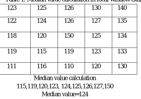
1) Median Filter: Median filter is the nonlinear filter. The main idea behind the median filter is to find the median value by across the window, replacing each entry in the window with the median value of the pixel

Table 1. Median value calculation in local window example

123 125 126 130 140

122 124 126 127 135

118 120 150 125 134

119 115 119 123 133

111 116 110 120 130

Median value calculation 115,119,120,123, 124,125,126,127,150

Median value=124

[41]The pattern of neighbor’s pixels is called the “window", when the window contains odd number of values in it then the median is simple: it is just the center value after all the entries in the window are sorted numerically in ascending order. But for an even number of entries, there is more than one center value; in that case the average of the two center pixel values is used. One of the major problems with the median filter is that it is relatively expensive and complex computation. For finding the median it is necessary to sort all the values in the neighborhood into numerical order and this filter relatively slow, even it is performed with fast sorting algorithms like quick sort. However the basic algorithm can be enhanced somewhat for the speed purpose.

3) Mean Filter: There are two types of filtering schemes namely linear filtering and nonlinear filtering. [43] Mean filter comes under linear filtering scheme. Mean filter is also known as averaging filter. The Mean Filter applies mask over each pixel in the signal. Each of the components of the pixels comes under the mask are being averaged together to form a single pixel that is why the filter is otherwise known as average filter. Edge preserving criteria is poor in mean filter. Mean filter is defined by

Mean filter (X1……XN….) = ∑

Where (x1 ….. xN) is image pixel range. Mean filter is useful for removing grain noise from the photography image. As each pixel gets summed the average of the pixels in its neighborhood is found out, local variations caused by grain noise are reduced considerably by replacing it with average value.

V. PROPOSED WORK

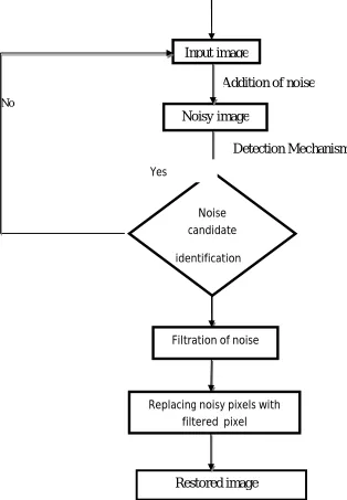
Here first an input image is taken .Then noise is added in that image .To identifying the noise candidate detection mechanism is used .After identifying the noise candidates the proposed filter is used for filtering the noisy candidates which is to be used to restore the noisy candidates to obtain the restored image.

No

Yes

Fig 5.Prposed work flow of the entire denoising Process

Restored image

Filtration of noise

Replacing noisy pixels with filtered pixel

Noisy image

Noise candidate

identification

Input image

Addition of noise

A. Proposed modified weighted mean filter

After detection, the next problem is how to choose an appropriate filter to remove these detected noisy pixels. Instead of using the existing median or mean filters [49, 29] proposed by F. Ahmed et.al, B.xiong et.al, in this section a more robust weighted mean filter (MWMF) is designed for image denoising. The weight in the proposed MWMF contains three components which take into account both the image features and IN characteristics. Hence it is more suitable for IN removal. Let Si,j be a set of pixel coordinates within a (2N+1) × (2N + 1)sliding window, centered at the (i,j)-th pixel. Suppose xi,j is the (i,j)-th pixel in the noisy image, and

is the output of the filter, then

= ∑_∑,€ , , , , ,

,

,€ , , ,

(9)

Where , is the distance weight inverse to the spatial distance between the neighbor pixel (i.e., ,) and the center one (i.e., , ). It is expected that the larger the distance between , and , is, the smaller the distance weight should be, and vice versa. Here,

, is simply defined as the inverse function of the spatial distance

,=_{( ) ( )} (10)

weight. On the contrast, if a pixel has a larger probability to be noise, the clean-like weight for it should be lower. Extremely, the noise free pixel has the largest weight, and the completely noisy pixel (the pixel with f value equals to 1) has no weight. Therefore, the clean-like weight is defined as,

W,=e| ( , ) |−1 (11)

And , is the median-similarity weight, which indicates that if the luminance intensity of , is closer to the median value of the relative-clean pixels (pixels with membership function f < 1), the median-similarity weight for , should be higher. The mathematical formula is defined as follows

W_,=e(

(| _, ∗ |)

)

(12)

in which ,( , )€ , /( , ) is the neighbor pixel of , in the sliding window, ∗ is the median value of the neighbor pixels excluded the noisy ones, i.e. ∗ = { ∗, }, denotes the set containing the relative clean pixels in the window.

X∗, = {x ,|(k, l)€S,, 0≤f(k, l) < 1} (13)

And =max {x , −x∗ |(k, l)€S,/(i, j)} is the maximum difference

The idea for designing such three components for the weight is quite simple. Firstly, it is well known that, in natural images, the closer the distance of two pixels is, the closer the relationship will be. Hence setting larger weights for these pixels that near to the current pixel is reasonable. Secondly, it is sensible just using these information pixels to filtering the noisy ones. Therefore, in the proposed weighted mean filter, the clean-like weight is inversely proportional to the membership function f. Finally, since median value is a good estimator for the IN, it is advisable to design large weights for these pixels whose luminance intensities are approach to the median value of the relative-clean ones.

B. Proposed Denoising algorithm

All the pixels in the image undergo testing for noise detection. A binary decision matrix is formed at the end of calculation. The decision matrix has values ‘1’ indicating corrupted and ‘0’ as uncorrupted. Further filtration of noisy pixels is done by storing value of X̂ in x(i,j) The size of input image X is denoted as P*Q. restored image Y.

1) Algorithm 1

a) Read noisy image X .

b) Initialize N=1,Threshold T=60; c) For every row i= 1 to P

d) For every column j= 1 to Q

e) Create rectangular 3×3 window around the noisy pixel and find ROAD values and compare with threshold T, update the binary noise matrix f.

g) End for row

h) for every row i=1 to P i) for every col j=1 to Q j) if X(i,j)==1

k) ifN<Nmax && <3 minimum clean pixel

l) X(row,col)= X̂ (i,j)

m) else

n) N=N+1

o) end if

p) end if

q) end for column r) end for row

VI. SIMULATION AND EXPERIMENTAL RESULTS

The simulation was carried out using MATLAB (Matrix laboratory) of R2014 version (8.3.0.532).Simulation work is implemented in windows-7 Home basic operating system, Intel(R) core(TM) i5 processor with processor speed 2.40 GHz, RAM 4 GB.

arameter requirement:

Threshold value (T=60)

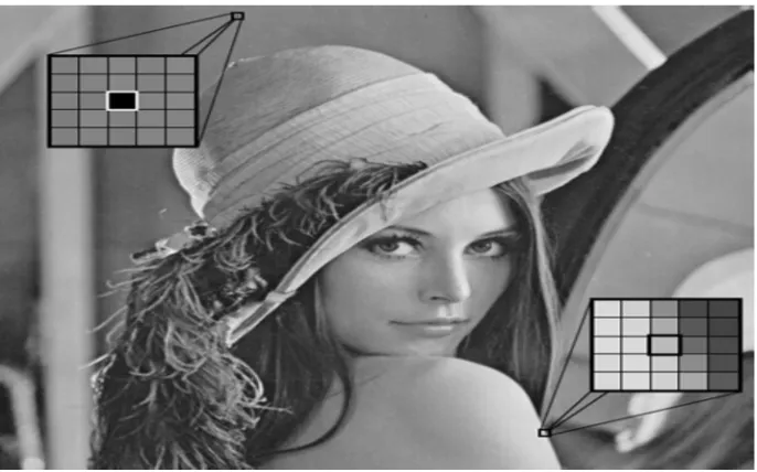
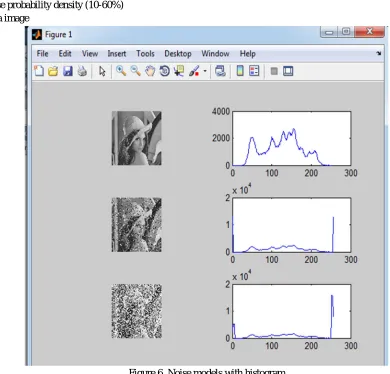
Local window (2N+1) × (2N+1) Noise probability density (10-60%) Lena image

Figure 6. Noise models with histogram

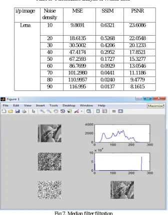
Table 2: Performance analysis of median filter i/p image Noise density MSE SSIM PSNR

Lena 10 3.0908 0.9779 36.2991

20 6.16 0.9176 29.945

30 10.3543 0.7412 23.8222 40 17.7079 0.4581 18.9251 50 28.1170 0.2276 15.1905 60 42.9959 0.1042 12.2415 70 60.4952 0.0526 9.9942 80 81.2169 0.0248 8.1140 90 104.7713 0.0122 6.6096 Table 3: Performance analysis of Weiner filter

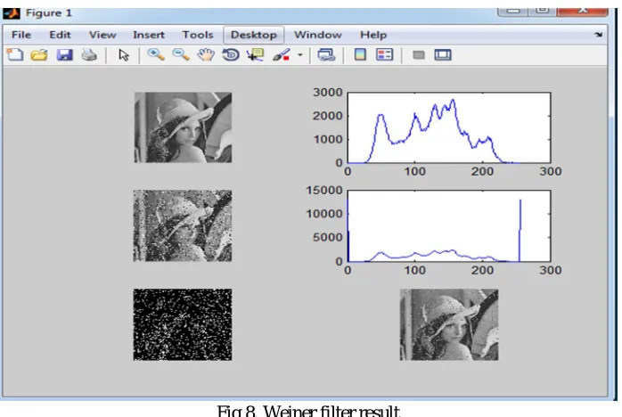
i/p image Noise density

MSE SSIM PSNR

Lena 10 9.8691 0.6321 23.6086

20 18.6135 0.5268 22.0548 30 30.5002 0.4206 20.1233 40 47.4174 0.2952 17.8521 50 67.2593 0.1727 15.3277 60 86.7699 0.0929 13.0546 70 101.2980 0.0441 11.1186 80 110.9957 0.0240 9.4779 90 116.995 0.0137 8.1615

Fig 7. Median filter filtration

Fig 8. Weiner filter result

Figure 7 shows Lena image as an input image added with 10% salt & pepper noise, detection is done by ROAD then filtered by Weiner filter and its Histogrammatical representation.

Fig 10 comparison result of SSIM

Fig 12. Comparison result of IEF

Noisy Image Added RVI Restored Image

10%

20%

40%

50%

60%

Fig 13.Shows the input and output image

Fig 13. Tells about Lena image taken as input image with 10-60% noise densities of RVIN and the restored image as output.

Table 4.Comparative data analysis of false alarm in different filters

Filter BRBDNR BDND NUASAM Proposed

Noise density (%) False alarm(FA)

10 29220 6350 1034 7

20 17857 9475 1164 6

30 9297 17538 1302 10

40 3737 32082 1881 22

50 1640 49010 3889 20

60 2964 61012 8539 32

Table 5.Comparative data analysis of missed detection in different filters

Filter BRBDNR BDND NUASAM Proposed

Noise density (%) Missed Detection (MD)

10 65 46 1640 0

20 557 531 3365 0

30 3141 2697 5108 1

40 18427 8110 7554 3

50 55788 18608 11720 12

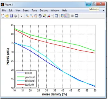
Table 6. PSNR (Peak signal to noise ratio comparison among filters) Noise

density

BRBDNR BDND NUASM Proposed

10 34.90982 35.33848 34.90982 42.93883

20 32.90524 30.72783 32.90524 39.5

30 27.04175 24.67717 27.04175 37.26798

40 19.17641 19.16315 19.17641 35.55494

50 14.15022 14.4636 14.15022 33.74834

60 11.34043 10.9053 11.34043 30.55413

Table.7 Comparison of FSIM among different filters

Noise density

BRBDNR BDND NUASM Proposed

10 0.989874 0.993766 0.998736 0.998882

20 0.988644 0.978919 0.996453 0.997345

30 0.968887 0.918668 0.993466 0.995225

40 0.853116 0.765014 0.989646 0.992557

50 0.685993 0.543291 0.982468 0.988568

60 0.575796 0.378226 0.974201 0.975818

Table. 8 Comparison of SSIM among different filters Noise

density

BRBDNR BDND NUASM Proposed

10 0.938448 0.978414 0.989383 0.990845 20 0.933684 0.934709 0.974178 0.980285 30 0.847472 0.789932 0.956825 0.968743 40 0.514154 0.527363 0.934284 0.955376 50 0.213544 0.228176 0.901006 0.937861 60 0.107106 0.078356 0.868631 0.90463

Table.9 Comparison of IEF among different filters Noise

density

BRBDNR BDND NUASM Proposed

VII.CONCLUSION

An image is an artifact that depicts visual perception. A digital image is a numeric representation (normally binary) of a two-dimensional image. Noise is the unwanted information present in image which degrades the quality of an image. Image denoising is the essential pre-processing step for image analysis. Previously filters were used to remove the noise which less efficiently worked for noise removal process but now a days noise removal carried out in two phases .First detection process carried out for finding the noise candidates, secondly filter out those noise candidate to obtain the restored image. In this thesis a modified weighted mean filter is used with noise detection scheme ROAD which better performs as comparison to other three types of denoising filtration scheme. A Lena image added with random valued (10-60)% noise density is tested by the above said filtration scheme performed well as comparison to other three existing filters BDND,NUASM,BRBDNR up to 60 % noise density .It has been concluded that the higher the PSNR,low MSE with less false hit and miss detection counts leads to better denoised image. Further research can be made to build more robust noise detection scheme along with better filtering technique for producing better denoised image.

REFERENCES

[1] R C Gonzalez and R E Woods. Digital Image Processing. Prentice-Hall, India, second edition, 2007.

[2] B Chandra and D Dutta Majumder. Digital Image Processing and Analysis. Prentice-Hall, India, first edition, 2007.

[3] K. S. Srinivasan and D. Ebenezer. A new fast and efficient decision based algorithm for removal of high-density impulse noises. IEEE Signal Process. Lett.,14(3):189-192,March2007.

[4] T. Chen and H. R. Wu. Adaptive impulse detection using center-weighted median filters. IEEE Signal Process. Lett., 8(1):1–3, January 2001 [5] J. Ko, Y.H. Lee, Center weighted median filters and their applications to image enhancement, IEEE Trans. Circ. Syst. 38 (9) (1991) 984–993.

[6] T. Chen and H. R.Wu. Space variant median filters for the restoration of impulse noise corrupted images. IEEE Trans. Circuits Syst. II, 48(8):784–789, August 2001

[7] K.-K. Ma T. Chen and L.-H. Chen. Tri-state median filter for image denoising.IEEE Signal Process. Lett, 8(12):1834–1838, December 1999. [8] V. Senk V. Crnojevic and Trpovski. Advanced impulse detection based on pixelwise mad. IEEE Signal Process. Lett, 11(7):589–592, July 2004. [9] S. K. Mitra E. Abreu, M. Lightstone and K. Arakawa. A new efficient approach forthe removal of impulse noise from highly corrupted images. IEEE

Trans. ImageProcessing, 5:1012–1025, June 1996.

[10] Y. Dong and S. Xu. A new directional weighted median filter for removal of random-valued impulse noise. IEEE Signal Process. Lett, 14(3):193–196, March

2007.

[11] S. Akkoul, R. Ledee, R. Leconge, R. Harba, A new adaptive switching median filter, IEEE Signal Process. Lett. 17 (6) (2010) 587–590.

[12] S.Esakkirajan, T.Veerakumar, AdabalaN.Subramanyam, C.H.PremChand, “Removal of High density Salt and Pepper Noise Through Modified Decision Based Unsymmetric Trimmed Median Filter,” IEEE Signal process. Lett., Vol. 18,no 5,May 2011

[13] Iyad F.Jafar, Rami A.AlNa’mneh and Khalid A.Darabkh, “Efficient Improvements on the BDND Filtering Algorithm for the Removal of High-Density Impulse Noise,” IEEE Transactions on Image Processing, vol.22, No. 3, (1223-1232).March 2013.

[14] Sruthi Ignatious, Robin Joseph, “Iterative Average Estimation Filter Using BDND algorithm for the removal of high density Impulse noise,”, International Journal of Computer Science and Mobile Computing (IJCSMC) Vol.2 Issue 13, December 2013.

[15] Ng, P.-E., Ma, K.-K., “ A Switching Median Filter with Boundary Discriminative Noise Detection for Extremely Corrupted Images, ”IEEE Transactions on Image Processing 15(6), 1506–1516 (2006)

[16] H. Hwang and R.A.Haddad, “Adaptive median filters: New algorithms and results,” IEEE Trans. Image Process., vol. 4, no. 4, pp. 499–502,1995. [17] Peixuan Zhang and Fang “A new adaptive weighted Mean filter for removing salt-and-pepper noise”,IEEE signal processing letters ,vol.21

NO.10,October 2014.

[18] M.Nasri,S.Saryazdi,H.Nezamabadi-pour,”SNLMal : A switching non-local means filter for removal of high density salt and peeper noise”,Department of Electrical engineering ,Shahid Bahonar University of Kerman,P.O.box 76169-133,Iran

[19] IyadF.Jafar, Rami A. AlNa’mneh, and Khalid A. Darabkh” Efficient Improvements on the BDND Filtering Algorithm for the Removal of High-Density Impulse Noise”

[20] Esakki rajan,S,Veerakumar,T.,Subramanyam,A.N and Premchand,C.h,”Removal of high density salt and peepper noise through modified decision based unsymmetric median filter”,IEEE signal processing letters,18(5),pp.287-29(2011)

[21] A.C Bovik ,Hand book of Image and Video Processing.New York ,NY,USA:Academic ,2000

[22] Dong ,Y,Chan ,R.H and Xu,S.”A detection statistics for random –valued impulse noise,”IEEE Transanctions on image processing ,16(4),pp 1112-1120(2007)

[23] Zhou, W. and Zhang,D,”Progressive switching median filter for the removal of impulse noise from highly corrupted images”,IEEE transanctions on circuit and systems II:Analog and Digital Signal processing ,46(1),pp.78-80(1999)

[24] P.-E. Ng and K.-K. Ma, “A Switching Median Filter With Boundary Discriminative Noise Detection for Extremely Corrupted Images,” IEEE Transactions on Image Processing, Vol. 15, No. 6, pp. 1506-1516, June 2006.

[26] Cheng-hsiung hsieh, Po-chin huang, and Sheng-yung hung,” Noisy Image Restoration Based on Boundary Resetting BDND and Median Filtering with Smallest Window” Department of Computer Science and Information Engineering Chaoyang University of Technology

[27] W. Luo, A new efficient impulse detection algorithm for the removal of impulse noise, IEICE Trans. Fund. Electron. Commun. Comput. Sci. 88 (10)551 (2005) 2579–2586.

[28] T. Sun, Y. Neuvo, Detail-preserving median based filters in image processing, Pattern Recogn. Lett. 15 (1994) 341–347.

[29] B. Xiong, Z. Yin, A universal denoising framework with a new impulse detector and nonlocal means, IEEE Trans. Image Process. 21 (4) (2012) 564 1675 [30] D.A.F. Florencio, R.W. Schafer, Decision-based median filter using local signal statistic, Proc. SPIE 2308 (1994) 268–275.

[31] E. Abreu, M. Lightstone, S.K. Mitra, K. Arakawa, A new efficient approach for the removal of impulse noise from highly corrupted images, IEEE Trans. Image Process. 5 (6) (1996) 012–1025.

[32] C.H. Lin, J.S. Tsai, C.T. Chiu, Switching bilateral filter with a texture/noise detector for universal noise removal, IEEE Trans. Image Process. 19 (9) (2010) 2307–2320.

[33] R. Garnett, T. Huegerich, C. Chui, W. He, A universal noise removal algorithm with an impulse detector, IEEE Trans. Image Process. 14 (11) (2005) 1747– 1754.

[34] H. Yu, L. Zhao, H. Wang, An efficient procedure for removing random-valued impulse noise in images, IEEE Signal Process. Lett. 15 (2008) 922–925. [35] U. Ghanekar, A.K. Singh, R. Pandey, A contrast enhancement-based filter for removal of random valued impulse noise, IEEE Signal Process. Lett. 17 (1)

536 (2010) 47–50.

[36] H.H. Tsai, B.M. Chang, X.P. Lin, Using decision tree, particle swarm optimization, and support vector regression to design a median-type filter with a 2- level impulse detector for image enhancement, Inf. Sci. 195 (2012) 103–123.

[37] T.C. Lin, Switching-based filter based on dempsters combination rule for image processing, Inf. Sci. 180 (24) (2010) 4892–4908

[38] A. Buades, B. Coll, J.M. Morel, A non-local algorithm for image denoising, in: IEEE Computer Society Conference on Computer Vision and Pattern Recognition, CVPR 2005, vol. 2, IEEE, 2005, pp. 60–65.

[39] H. Hu, B. Li, Q. Liu, Removing mixture of gaussian and impulse noise by patch-based weighted means, arXiv preprint arXiv:1403.2482, 2014. [40] J. Delon, A. Desolneux, A patch-based approach for removing impulse or mixed gaussian-impulse noise, SIAM J. Imaging Sci. 6 (2) (2013) 1140–1174. [41] James C. Church, Yixin Chen, and Stephen V. Rice Department of Computer and InformationScience, University of Mississippi, “A Spatial Median Filter

for Noise Removal in Digital Images”, IEEE, page(s): 618- 623, 2008.

[42] G.Shi Zhong, “Image De-noising using Wavelet Thresholding and Model Selection”,Image Processing, 2000, Proceedings, 2000 International Conference on, Volume: 3, 10-13

[43] Gajanand Gupta, “Algorithm for Image Processing Using Improved Median Filter andComparison of Mean, Median and Improved Median Filter” (IJSCE) ISSN: 2231-2307,Volume-1, Issue-5, November 2011.

[44] Charles Boncelet, “Image Noise Models” in Alan C.Bovik, Handbook of Image and Video Processing, 2005 [45] P.Y. Chen, C.Y. Lien, “An efficient edge-preserving algorithm for removal of

salt-and-pepper noise”, IEEE Signal Processing Letters 15, 833–836, 2008.

[46] M. Rosa-Zurera, A.M. Co´breces-A´lvarez, J.C. Nieto-Borge, M.P. Jarabo-Amores, and D.Mata-Moya. “Wavelet denoising with edge detection for speckle reduction in SAR images” EUSIPCO Poznon, 2007

[47] Sedef Kent, Osman Nuri Oçan, and Tolga Ensari, "Speckle Reduction of Synthetic Aperture Radar Images Using Wavelet Filtering", in Astrium EUSAR 2004 Proceedings, 5th European Conference on Synthetic Aperture Radar, May25–27, 2004, Ulm, Germany, 2004

[48] T.C. Lin, A new adaptive center weighted median filter for suppressing impulsive noise in images, Inf. Sci. 177 (4) (2007) 1073–1087.