NP Bracketing by Maximum Entropy Tagging and SVM Reranking

NP Bracketing by Maximum Entropy Tagging and SVM Reranking

Hal Daum´e III and Daniel Marcu

University of Southern California Information Sciences Institute 4676 Admiralty Way, Suite 1001

Marina del Rey, CA 90292 {hdaume,marcu}@isi.edu

Abstract

We perform Noun Phrase Bracketing by using a lo-cal, maximum entropy-based tagging model, which produces bracketing hypotheses. These hypothe-ses are subsequently fed into a reranking frame-work based on support vector machines. We solve the problem of hierarchical structure in our tag-ging model by modeling underspecified tags, which are fully determined only at decoding time. The tagging model performs comparably to competing approaches and the subsequent reranking increases our system’s performance from an f-score of81.7to 86.1, surpassing the best reported results to date of 83.8.

1 Introduction and Prior Work

Noun Phrase Bracketing (NP Bracketing) is the task of identifying any and all noun phrases in a sen-tence. It is a strictly more difficult problem than NP Chunking (Ramshaw and Marcus, 1995), in which only non-recursive (or “base”) noun phrases are identified. It is simultaneously strictly more sim-ple than either full parsing (Collins, 2003; Charniak, 2000) or supertagging (Bangalore and Joshi, 1999). NP Bracketing is both a useful first step toward full parsing and also a meaningful task in its own right; for instance as an initial step toward co-reference resolution and noun-phrase translation.

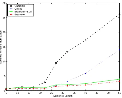
While existing NP Bracketers (including the one described in this paper) tend to achieve worse over-all F-measures than a full statistical parser (eg., (Collins, 2003; Charniak, 2000)), they can be sig-nificantly more computationally efficient. Statisti-cal parsers tend to sStatisti-cale exponentially in sentence length, unless a narrow beam is employed, which leads to globally poorer parses. In contrast, the bracketer described in this paper scales linearly in

[[Confidence] in [the pound]] is widely expected to take [another sharp dive] if [[[trade figures] for [September]] , due for [release] [tomorrow] ,] . . .

Figure 1: Sample sentence with NPs bracketed.

the length of the sentence to find the globally op-timal solution. This trade-off is depicted graphi-cally in Figure 2. This figure shows the amount of time (excluding any startup overhead) spent pars-ing or bracketpars-ing uspars-ing this system (the two lowest lines) versus the parsers of Collins (2003) and Char-niak (2000) run with default settings.

NP Bracketing was the shared task of the Com-putational Natural Language Learning workshop in 1999 (CoNLL-99). In this competition, NP Brack-eting systems were trained on sections 15-18 of the Wall Street Journal corpus, while section 20 was used for testing. The bracketing information was extracted directly from the Penn Treebank, essen-tially disregarding all non-NP brackets. An example bracketed sentence is in Figure 1.

There have been several successful approaches reported in the literature to solve this task. Tjong Kim Sang (1999) first used repeated chunking to at-tain an f-score of82.98 during the CoNLL compe-tition and subsequently (Sang, 2002) an f-score of 83.79using a combination of two different systems. Krymolowski and Dagan (2000) have obtained sim-ilar results using more training data and lexicaliza-tion. Brandts (1999) has used cascaded HMMs to solve the NP Bracketing problem; however, he eval-uated his system only on German NPs, so his results cannot be directly compared.

5 10 15 20 25 30 35 40 45 50 55 0

5 10 15 20 25 30

Sentence Length

Seconds to Parse (normalized)

Charniak Collins Bracketer+SVM Bracketer

Figure 2: Speed of different systems

form of a tree structure. Most solutions to prob-lems involving building trees from sequences build in to the model a concept of depth (in parsing, this is typically in the form of a chart; in bracketing and shallow parsing, this is typically in the form of em-bedded finite-state automata). We elect to take a completely different approach. The model we use is agnostic to any sort of depth: it hypothesizes un-derspecified tags and allows the matching bracket constraint to select a solution.

Specifically, we approach the NP Bracketing problem as a tagging and reranking problem. We use an efficient maximum entropy-based tagger to hypothesize possible bracketings (see Section 2) and then rerank these hypotheses using a support vector reranking system (see Section 3). Using only the tagger (without reranking), we achieve compa-rable results to those referenced above and, with the addition of the reranking system, achieve, to our knowledge, the best reported results to date.

2 Bracketing as a Tagging Problem

In any tagging problem, the task is to associate each word in the input with a single tag. There are many competing approaches to tagging problems including Hidden Markov Models (HMMs), Maxi-mum Entropy Markov Models (MEMMs) and Con-ditional Random Fields (CRFs). We adopt a slight variant of the MEMM framework.

2.1 Maximum Entropy Tagging Model

In the formulation of the maximum entropy tagging model, we assume that the probability distribution of tags takes the form of an exponential distribution, parameterized by a sequence of feature weights,

λm1 , where there are m-many features. Thus, we

obtain a distribution for P rλm

1 (ti ti−1,w¯) of the

form:

1

Zti−1,w¯

exp 



m

X

j=1

λjfj(ti, ti−1,w¯) 

 (1)

whereZti−1,w¯is a normalizing factor.

Like other maximum entropy approaches, this distribution is unimodal and optimal values for the

λs can be found through various algorithms; we use GIS. A good introduction to maximum entropy models can be found in (Berger et al., 1996).

In our approach, we use a tag set of exactly five tags: {open, close, in, out, sing}. Anopentag is assigned to all words that open a bracketing (regard-less of the number of brackets opened) and do not also close a bracketing. Aclosetag is assigned to all words that close a bracketing and do not also open one. Anintag is assigned to all words enclosed in an NP, but which neither open nor close one. Anout

tag is assigned to all words which are not enclosed in an NP. Asing(leton) tag is assigned to all words that both open and close a bracketing (regardless of whether they open or close more than just their own bracketing).

Note that such a tagging does not uniquely deter-mine a bracketing. For instance, the tag sequence

hsing singi could correspond either to[[w1] [w2]]

or to[w1] [w2]. Nevertheless, due to the constraints involved in the tagging process (namely that a close tag cannot appear unless one is already within an NP and that one cannot have two close tags when the corresponding open tags appear at the same lo-cation1), we hope that our system will be able to dis-ambiguate sufficiently. In other words, although our taggings are under-specified, we hope that the ad-ditional constraints that we subsequently associate with these tags will yield high quality bracketings.

2.2 Feature Functions

The probability distribution shown in Equation 1 is based onm-many real-valued feature functions,fj.

We use two classes of features, closed features and

open features (these roughly correspond to whether

they look at closed class elements or open class ele-ments). The open features for positioniare applied at positionsi,i−1andi+ 1. The closed features are applied ati,i−1,i−2,i−3andi+ 1,i+ 2 andi+ 3.

1

For instance, the bracketing[[w_i. . . w_j]] is disallowed;

Closed features include: part of speech tag (ac-cording to Brill’s (1995) tagger); two character suf-fix of word; first character of part of speech; initial character capitalized; word fully capitalized; last character is period; word position in sentence; and two features for when the word is either the first or last word in the sentence. Open features include: the word itself; the word lower-cased; the lower-cased stem (Porter, 1980); the lower-cased stem plus the part of speech; and 3 features that are each true when there is a CCin the next 2 through 5 words. In addition, we include a feature for tagti−1.

2.3 Maximum Entropy Training

We used generalized iterative scaling to train the maximum entropy model2 on929,921features and 211,728 training instances from sections 15-18 of the Penn Treebank (20% of which was set aside as a validation set). Training was run for ten thousand iterations and, at convergence, achieved a tagging error rate of2.1%on the training data and6.9%on the validation data.

2.4 Decoding Algorithm

We use a Viterbi-like dynamic programming de-coding algorithm, where transition probabilities are governed by the discriminative tagging model. However, the tags generated by our decoder are not the same as those predicted by the maximum en-tropy model. Our decoder does not search in the original space of tags (sing, in, out, . . .) but rather in a new space that yields only well-formed brack-etings. In the secondary search space, the algorithm is guaranteed to find the most likely well-formed bracketing, even though this might not correspond to the most likely tag sequence. While it would be possible to simply tag using the original tag set and allow the reranker (see Section 3) to select a well-formed bracketing, it is unlikely that this will lead to improved performance: the complexity of the de-coders will be the same, yet the bracketer would have to wade through significantly more bad tag-gings to find a good solution.

Our decoding tags take one of five forms, capi-talized to distinguish them from the maximum en-tropy tags: On, Cn, N,OnC,OCn wheren ≥ 1

for all butOCn wheren ≥ 2. The meaning of the

tags is: On means n simultaneous open brackets:

Cnmeansnsimultaneous close brackets. N means

that no brackets appear at this position. OnC

corre-2

Using the YASMET maximum entropy training package:

http://www.isi.edu/˜och/YASMET/.

0 20 40 60 80 100 120 140 160 180 200 82

84 86 88 90 92 94 96 98

Precision Recall F−Score

Figure 3: Plot ofnversus maximal f-score (and as-sociated precision and recall) for test data.

sponds to n open brackets and one close bracket, while OCn corresponds to one open bracket and

n ≥ 2 close brackets. These tags are enough to decode any well-formed bracketing.

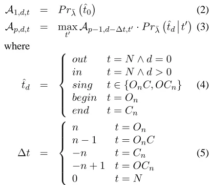
Our decoder assumes a maximum depth of tags

dhas been prespecified and then solves a dynamic programming problem on an n× d ×t array A, wherenis the sentence length andtdenotes an inte-ger corresponding to the highest possible decoding tag in an enumeration. The valueAi,d,t stores the

probability of being at position i and depth d af-ter applying tagtat that position. It is always the case thatt ≤ 4d. The time and space complexity of this decoding problem is thusO(d2n). The dy-namic programming problem is:

A1,d,t = P r_λ¯ tˆ0 (2)

Ap,d,t = max

t0 Ap−1,d−∆t,t0·P r

¯

λ ˆtd t0

(3)

where

ˆ

td =

     

    

out t=N∧d= 0

in t=N∧d >0

sing t∈ {OnC, OCn}

begin t=On

end t=Cn

(4)

∆t =      

    

n t=On

n−1 t=OnC

−n t=Cn

−n+ 1 t=OCn

0 t=N

(5)

The intuition for calculating the value of Ap,d,t

forp > 1(see Equation 3) is that we first choose

t and d, we can calculate the depth (d −∆t, see Equation 5) we must have been at previously. Thus, we must take the value ofAp−1,d−∆t,t0which is the

probability of having arrived at position p−1 at depth d −∆t with tag t0_{. We then multiply this} by the probability of getting from that position to the current position, which is given byP r¯_λ ˆt_d t0 (note that the normalization occurs over the new space of tags). The optimal tagging is given by back-tracing throughA, beginning atAn,0,tfor any

tag t. Even for long sentences, this algorithm re-quires very little time and memory.

2.5 Model Deficiencies

While the bracketing model described above al-ready performs comparably to competing ap-proaches (see Section 4), it is still subject to mak-ing categorical mistakes. Most of its errors are due to the locality of the decisions made. Because of the coarseness of the tags used in the maximum en-tropy tagging framework, the model is unable to dis-criminate between some bad bracketings and some good ones. For instance, it must assign precisely the same probability to both of the following brack-etings, since the maximum entropy tags (shown be-neath) are identical:

[[John,] [president] of [the company] ,] [[John,] [[president]of [the company]]],]

sing sing in open close close

This limitation causes the model to make con-sistent mistakes distinguishing between, for exam-ple, lists and appositional phrases. To solve these problems in the tagging model would be nearly im-possible, without giving up on efficiency. However, our decoder is able to producen-best lists using ex-act A∗ _{search that very frequently contain globally} superior taggings, even though the simple tagging model cannot recognize them as such.

In Figure 3, we show the maximal f-score (and corresponding precision and recall) for the best bracketing chosen out of the n-best, as we let n

range from 1 to 400 for both the validation data and the test data. As we can see from these graphs, we have the possibility of improving our system’s f-score performance by about ten points – from 82% to 93%, simply by being able to choose the correct hypothesis from the n-best list; also working with 100-best lists is likely sufficient.

3 Hypothesis Reranking

In the previous section, we described a tagging model for NP Bracketing that can produce n-best lists. In this section, we describe a machine learn-ing method for reranklearn-ing these lists in an attempt to choose a hypothesis which is superior to the first-best output of the decoder. Reranking ofn-best lists has recently become popular in several natural lan-guage problems, including parsing (Collins, 2003), machine translation (Och and Ney, 2002) and web search (Joachims, 2002). Each of these researchers takes a different approach to reranking. Collins (2003) uses both Markov Random Fields and boost-ing, Och and Ney (2002) use a maximum entropy ranking scheme, and Joachims (2002) uses a sup-port vector approach. As SVMs tend to exhibit less problems with over-fitting than other competing ap-proaches in noisy scenarios, we also adopt the sup-port vector approach.

3.1 Support Vector Reranking

A support vector classifier is a binary classifier with a linear decision boundary. The selected decision boundary is a hyperplane that is chosen in such a way that the distance between it and the nearest data points is maximized. Slack variables are commonly introduced when the problem is not linearly separa-ble, leading to soft margins.

For reranking, we assume that instead of having binary classes for theyis, we have real values which

specify the relative ordering (higher values come first). For this task, we get the following optimiza-tion problem (Joachims, 2002):

minimize 1 2||w¯||

2 +C

N

X

i=1

ξi,j (6)

subject to w¯·x¯i ≥w¯·x¯j + 1−ξi,j (7)

ξi,j ≥0 (8)

Where thei, js are drawn from comparable data points andyi ≥yj andCis a regularization

param-eter that specifies how great the cost of mis-ordering is. As noticed by Joachims, the condition in Equa-tion 7 can be reduced to the standard SVM model by subtractingw¯·¯xj from both sides.

3.2 Reranking Feature Functions

our own (those which are copied from Collins are marked with an asterisk). We view the hypothesized bracketing as a tree in a context free grammar and include features based on each rule used to gener-ate the given tree. For concreteness, we will use the CFG ruleNP→DT JJ NP(where theNPis selected as the head) as an example.

Rules*: the full CFG rule; in this case, the active rule would beNP→DT JJ NP.

Markov 2 Rules: CFG rules where 2-level Markovization has been applied. That is, we look at the rule for generating the first two tags, then the next two (given the previous one), then the next two (given the previous one), and so on. A start of branch tag ([S]) and end of branch tag ([/S]) are added to the beginning and end of the children lists. In this case, the rules that fire are: NP! →[S] DT, NP![S]→DT JJ,NP!DT→JJ NPandNP!JJ→NP [/S]. The notation isX!Y→A B, whereXis the true parent,Ywas the previous child in the Markoviza-tion, andA Bare the two children.

Lex-Rules*: full CFG rules, where terminal POS tags are replaced with lexical items.

Markov 2 Lex-Rules: Markov 2-style rules, ter-minal POS tags are replaced with lexical items.

Bigrams*: pairs of adjacent tags in the CFG rule; in our example, the active pairs are ([S],DT), (DT,JJ), (JJ,NP) and (NP,[/S]).

Lex-Bigrams*: same as BIGRAMS, but with lex-ical heads instead of POS tags.

Head Pairs*: pairs of internal node tags with the head type; in the example, (DT,NP), (JJ,NP) and (NP,NP).

Sizes: the child count, conditioned on the internal tag; eg.,NP→3.

Word Count: pair of the SIZESand total number of words under this constituent.

Boundary Heads: pairs of the first and last head in the constituent.

POS-Counts: a scheme of features that count the number of children whose part of speech tag matches a given predicate. There are six of these: (1) children whose tag begins with N, (2) children whose tag begins withNbut is notNP, (3) children which areDTs, (4) children whose tag begin withV, (5) children which are commas, (6) children whose tag isCC. In this case, we get a count of 1 for rules (2) and (3), and 2 for rule (1).

Lex-Tag/Head Pairs: same as HEAD PAIRS, but where lexical items are used instead of POS tags.

Special Tag Pairs: count of the lexical heads to the left and right of leaves tagged with each ofPOS, CC,INandTO.

Tag-Counts: another schema of features that replicates some of the features used in the maxi-mum entropy tagger. This schema includes all the original maximum entropy tags, as well as a feature for each maximum entropy tag at position i, paired with (a) the part of speech tag at positioni,i−1and

i+ 1, (b) the word at positioni,i−1andi+ 1, (c) the part of speech + word pair at those positions, (d) the maximum entropy tag at that position.

3.3 SVM Training

We develop three reranking systems, differentiated by the amount of training data used. The first, RR1, is trained on the validation part of the train-ing set (20% of sections 15-18). The second, RR2. is trained on the entire training set through cross-validation (all of sections 15-18). The final, RR3 is trained on the entire Penn Treebank corpus, except section 20.

Training the reranking system only on the valida-tion data (RR1) results in only a marginal gain of overall f-score, due primarily to the fact that most of the features use lexical information to prefer one bracketing over another. The validation data from sections 15-18 gives rise to2,012training instances and362,415features. In order to train the reranking system on all of the training data (RR2), we built five decoders, each with a different20%of the train-ing data held out. Each decoder is then used to tag the held-out20%(this is done so that the tagger does not do “too well” on its training data). This leads to 8,935sentences for training, with a total of1.1 mil-lion features. Training on all the WSJ data except section 20 (RR3) gives rise to 39,953 training in-stances and a total of just over 2.1million features. These examples give1,462,568rank constraints.

4 Results

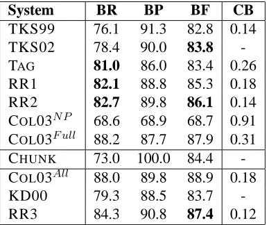
System BR BP BF CB TKS99 76.1 91.3 82.8 0.14 TKS02 78.4 90.0 83.8 -TAG 81.0 86.0 83.4 0.26 RR1 82.1 88.8 85.3 0.18 RR2 82.7 89.8 86.1 0.14 COL03N P 68.6 68.9 68.7 0.91 COL03F ull 88.2 87.7 87.9 0.31 CHUNK 73.0 100.0 84.4 -COL03All 88.0 89.8 88.9 0.18 KD00 79.3 88.5 83.7 -RR3 84.3 90.8 87.4 0.12

Table 1: Results on test data. The systems in the lower half are not directly comparable, since they were either trained or tested on different data.

In the table, TKS99 and TKS02 are the sys-tems of Tjong Kim Sang (1999; 2002). KD00 is the system of (Krymolowski and Dagan, 2000). All the COL03 systems are results obtained using the restriction of the output of Collins (2003) parser. In particular, the two comparable numbers coming from Collins’ parser are COL03N P and COL03F ull. The difference between these two systems is that the NP system is trained on parse trees, with all non-NP nodes removed. The FULLsystem is trained on full parse trees, and then the output is reduced to just in-clude NPs. COL03Allis trained on sections 2-21 of WSJ and tested on section 23, and is thus an upper bound, since these numbers are testing on training data.3 _{Our RR3 system had the reranking}

compo-nent (but not the tagging compocompo-nent) trained on all of the WSJ except for section 20.

The CHUNK row in the results table is the per-formance of an optimally performing NP chunker. That is, this is the performance attainable given a chunker that identifies base NPs perfectly (at100% precision). However, since this hypothetical sys-tem only chunks base NPs, it misses all non-base NPs and thus achieves a recall of only73.0, yield-ing an overall F-score below our system’s perfor-mance. Note also that no chunker will perform this well. Current systems attain approximately 94% precision and recall on the chunking task (Sha and Pereira, 2002; Kudo and Matsumoto, 2001), so the

3

Collins independently reports a recall of91.2and

preci-sion of90.3for NPs (Collins, 2003); however, these numbers

are based on training on all the data and testing on section 0. Moreover, it is possible that his evaluation of NP bracketing is not identical to our own. The results in row COL03F ull are therefore perhaps more relevant.

actual performance for a real system would be sub-stantially lower.

The four criteria these systems are evaluated on are bracketing recall (BR), bracketing precision (BP), bracketing f-score (BF) and average crossing brackets (CB). Some systems do not report their crossing bracket rate. All of these metrics are cal-culated only onNP*andWHNP*brackets.

5 Comparison of Performance

The results depicted in Table 1 show that, when comparing our system directly to Collins’ parser, his system tends to achieve significantly higher lev-els of recall, while maintaining a slight advantage in terms of precision. This table, however, does not tell the full story. As is typically observed in these sort of applications, it is not the case that Collins’ parser is “winning” by a little on all the data, but rather that Collins’ parser wins on some of the data and our bracketer wins on some of the data. In this section, we analyze the differences.

Overall, there are 2,012 sentences in the test data. In558cases, both the bracketing system and Collins’ parser achieve perfect precision. In 505 cases, both achieve perfect recall. For the remainder of the discussion in this section, when discussing precision, we will only consider the cases in which not both achieved perfect scores, and similarly for recall.

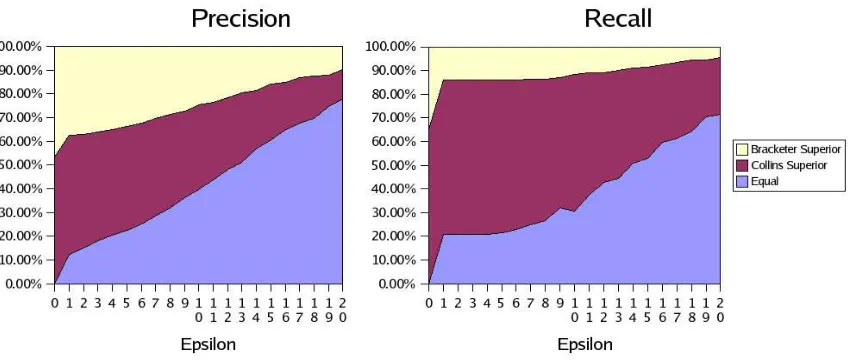
In Figure 4, we depict (excluding the mutually perfect sentences) the percentage of sentences on which each system is better than the other by a dis-tance of at least. Along the X-axes, the value of

ranges from0to20. At a given value of, the seg-mentation along the Y-axes depict (a) along the top (in yellow where available), the proportion of sen-tences for which the bracketer’s precision (for the left hand image) was at least of that of Collins’; (b) in the middle (in red), the proportion of sen-tences for which Collins’ was at leastbetter; and (c) along the bottom (in blue), the proportion of sen-tences where the two systems performed withinof each other.

How-Figure 4: Proportion of sentences for which one system outperforms the other with difference at least.

Precision Recall Tag RR2 COL03 RR2 COL03 NP 21.4 19.8 20.5 21.3 VP 7.49 8.52 8.31 7.57 NN 8.22 7.62 7.43 7.83 IN 6.01 5.89 5.31 6.15 PP 5.90 5.63 5.16 6.03 S 4.96 5.82 5.44 5.15 NNP 6.15 4.79 6.29 5.82

Table 2: Percentage of tags on superior system.

ever, in contrast to the Precision graph, for the first 10or so values of, these proportions remain roughly the same (in fact, for a short period, Collins’ actually looses ground). This suggests that there are a relatively large proportion of sentences for which our system is performing abominably (with > 10 recall points difference) in comparison to Collins’. However, once a critical mass of >10is reached, the relative differences become less strong.

Since neither system is winning in all cases, in an effort to better understand the conditions in which one system will outperform the other, we inspect the sentences for which there was a difference in performance of at least10(for precision and recall separately). To perform this investigation, we look at the distribution of tags in the true, full parse trees for those sentences. These percentages, for the 7 most common tags, are summarized in Table 2 (for example, the relative frequency of the NP tag in sen-tences where the RR2 system achieved higher pre-cision was 21.4, while for the sentences for which COL03 achieved higher precision was 19.8).

The first thing worth noticing in this table is that

in general, when one system achieves higher preci-sion, the other system achieves higher recall, which is not surprising. However, in the last row, corre-sponding to proper nouns, the RR2 system outper-forms the COL03 (this is the “Full” implementa-tion) in both precision and recall, suggesting that our system is better able to capture the phrasing of proper nouns. We attribute this to the fact that our model is specialized to identify noun phrases, of which proper nouns comprise a large part. Simi-larly, the largest gains in recall for COL03 over RR2 are in sentences with many PPs. This coincides with our intuition about the syntactic parser being better able to capture long, embedded noun phrases.

6 Conclusion

We have presented a method for performing noun phrase bracketing, which outperforms competing methods both in terms of f-score and recall. The system is based on two separate components: a maximum entropy-based tagging system and a sup-port vector machine reranking system. The key component of the tagging system is that it produces underspecified tags that are determined only at de-coding time by bracketing constraints. The tagging system operates very quickly and can tag and rerank at a rate of approximately two sentences per second. The tagger alone achieves an f-score of83.4. This score is only0.4%lower (absolute) than the best re-ported result to date of83.8.

im-proving our performance beyond the best reported system to date.

As we can see from Table 1, by comparing the output of our system to that of COL00F ull, there is much in the way of recall to be gained by using a full syntactic parser. However, this gain comes at two expenses. First, full syntactic parsers are com-putationally more expensive to run. Moreover, per-formance of Collins’ parser degrades significantly (from 87.9 to 68.7 in f-score) when it cannot take advantage of other constituent information. This has a strong influence when one is faced with the task of moving to a new domain. On the one hand, our system (as well as the other bracketing systems cited) requires data to only be annotated at the NP level in order to achieve high performance. Con-versely, without full parses, using a parser for learn-ing NPs is inadequate.

Despite these successes, there is still much that can be improved upon. While the reranking is very efficient in the classification phase, training a support vector reranking system is computation-ally very expensive. Other well grounded statistical learning systems might allow us to train this com-ponent on more data and using more features. We also hope to be able to improve our system’s perfor-mance from its current rate of86.1(on official data) and 87.4 (on all data) closer to then-best optimal, depicted in Figure 3.

7 Acknowledgments

This work was partially supported by DARPA-ITO grant N66001-00-1-9814, NSF grant IIS-0097846, and a USC Dean Fellowship to Hal Daum´e III.

References

Srinivas Bangalore and Aravind K. Joshi. 1999. Supertagging: An approach to alsmost parsing.

Computational Linguistics, 25(2):237–265.

Adam L. Berger, Stephen A. Della Pietra, and Vin-cent J. Della Pietra. 1996. A maximum entropy approach to natural language processing.

Com-putational Linguistics, 22(1):39–71.

Thorsten Brandts. 1999. Cascaded markov models. In Proceedings of EACL 1999.

Eric Brill. 1995. Transformation-based error-driven learning and natural language processing: a case study in part of speech tagging.

Computa-tional Linguistics, December.

Eugene Charniak. 2000. A maximum-entropy-inspired parser. In Proceedings of the First

An-nual Meeting of the North American Chapter

of the Association for Computational Linguistics NAACL–2000, pages 132–139, Seattle,

Washing-ton, April 29 – May 3.

Michael Collins. 2003. Head-driven statistical models for natural language parsing.

Computa-tional Linguistics, 29(4), December.

Thorsten Joachims. 2002. Optimizing search en-gines using clickthrough data. In Proceedings of

the ACM Conference on Knowledge Discovery and Data Mining (KDD). ACM.

Yuval Krymolowski and Ido Dagan. 2000. Incorpo-rating compositional evidence in memory-based partial parsing. In Proceedings of ACL 2000, Hong Kong.

Taku Kudo and Yuji Matsumoto. 2001. Chunking with support vector machines. In NAACL. Franz Josef Och and Hermann Ney. 2002.

Discrim-inative training and maximum entropy models for statistical machine translation. In ACL 02, pages 295–302, Philadelphia, PA, July.

M.F. Porter. 1980. An algorithm for suffix strip-ping. Program, 14:130–137.

Lance A. Ramshaw and Michell P. Marcus. 1995. Text chunking using transformation-based learn-ing. In Proceedings of the Third ACL Workshop

on Very Large Corpora. Association for

Compu-tational Linguistics.

Erik F. Tjong Kim Sang. 1999. Noun phrase detec-tion by repeated chunking. In CoNLL-99

Work-shop, Bergen, Norway.

Erik F. Tjong Kim Sang. 2002. Memory-based shallow parsing. Journal of Machine Learning

Research, 2:559 – 594, March.

Fei Sha and Fernando Pereira. 2002. Shallow pars-ing with conditional random fields. In