Efficient Incremental Decoding for Tree-to-String Translation
Liang Huang1
1Information Sciences Institute
University of Southern California 4676 Admiralty Way, Suite 1001 Marina del Rey, CA 90292, USA
{lhuang,haitaomi}@isi.edu
Haitao Mi2,1
2Key Lab. of Intelligent Information Processing
Institute of Computing Technology Chinese Academy of Sciences P.O. Box 2704, Beijing 100190, China
Abstract
Syntax-based translation models should in principle be efficient with polynomially-sized search space, but in practice they are often embarassingly slow, partly due to the cost of language model integration. In this paper we borrow from phrase-based decoding the idea to generate a translation incrementally left-to-right, and show that for tree-to-string models, with a clever encoding of deriva-tion history, this method runs in average-case polynomial-time in theory, and linear-time with beam search in practice (whereas phrase-based decoding is exponential-time in theory and quadratic-time in practice). Exper-iments show that, with comparable translation quality, our tree-to-string system (in Python) can run more than 30 times faster than the phrase-based system Moses (in C++).
1 Introduction
Most efforts in statistical machine translation so far are variants of either phrase-based or syntax-based models. From a theoretical point of view, phrase-based models are neither expressive nor efficient: they typically allow arbitrary permutations and re-sort to language models to decide the best order. In theory, this process can be reduced to the Traveling Salesman Problem and thus requires an exponential-time algorithm (Knight, 1999). In practice, the de-coder has to employ beam search to make it tractable (Koehn, 2004). However, even beam search runs in quadratic-time in general (see Sec. 2), unless a small
distortion limit (say,d=5) further restricts the possi-ble set of reorderings to those local ones by ruling out any long-distance reorderings that have a “jump”
in theory in practice
phrase-based exponential quadratic tree-to-string polynomial linear
Table 1: [main result] Time complexity of our incremen-tal tree-to-string decoding compared with phrase-based. In practice means “approximate search with beams.”
longer than d. This has been the standard prac-tice with phrase-based models (Koehn et al., 2007), which fails to capture important long-distance re-orderings like SVO-to-SOV.
Syntax-based models, on the other hand, use syntactic information to restrict reorderings to a computationally-tractable and linguistically-motivated subset, for example those generated by synchronous context-free grammars (Wu, 1997; Chiang, 2007). In theory the advantage seems quite obvious: we can now express global reorderings (like SVO-to-VSO) in polynomial-time (as opposed to exponential in phrase-based). But unfortunately, this polynomial complexity is super-linear (being generally cubic-time or worse), which is slow in practice. Furthermore, language model integration becomes more expensive here since the decoder now has to maintain target-language boundary words at
both ends of a subtranslation (Huang and Chiang,
2007), whereas a phrase-based decoder only needs to do this at one end since the translation is always growing left-to-right. As a result, syntax-based models are often embarassingly slower than their phrase-based counterparts, preventing them from becoming widely useful.
Can we combine the merits of both approaches? While other authors have explored the possibilities
of enhancing phrase-based decoding with syntax-aware reordering (Galley and Manning, 2008), we are more interested in the other direction, i.e., can syntax-based models learn from phrase-based de-coding, so that they still model global reordering, but in an efficient (preferably linear-time) fashion?
Watanabe et al. (2006) is an early attempt in this direction: they design a phrase-based-style de-coder for the hierarchical phrase-based model (Chi-ang, 2007). However, this algorithm even with the beam search still runs in quadratic-time in prac-tice. Furthermore, their approach requires grammar transformation that converts the original grammar into an equivalent binary-branching Greibach Nor-mal Form, which is not always feasible in practice.
We take a fresh look on this problem and turn our focus to one particular syntax-based paradigm, tree-to-string translation (Liu et al., 2006; Huang et al., 2006), since this is the simplest and fastest among syntax-based approaches. We develop an incremen-tal dynamic programming algorithm and make the following contributions:
• we show that, unlike previous work, our in-cremental decoding algorithm runs in average-case polynomial-time in theory for tree-to-string models, and the beam search version runs in linear-time in practice (see Table 1);
• large-scale experiments on a tree-to-string sys-tem confirm that, with comparable translation quality, our incremental decoder (in Python) can run more than 30 times faster than the phrase-based system Moses (in C++) (Koehn et al., 2007);
• furthermore, on the same tree-to-string system, incremental decoding is slightly faster than the standard cube pruning method at the same level of translation quality;
• this is also the first linear-time incremental de-coder that performs global reordering.
We will first briefly review phrase-based decod-ing in this section, which inspires our incremental algorithm in the next section.
2 Background: Phrase-based Decoding
We will use the following running example from Chinese to English to explain both phrase-based and syntax-based decoding throughout this paper:
0B`ush´ı1 Bush
yˇu2 with
Sh¯al´ong3 Sharon
jˇux´ıng4 hold
le -ed
5hu`ıt´an6 meeting
‘Bush held talks with Sharon’
2.1 Basic Dynamic Programming Algorithm
Phrase-based decoders generate partial target-language outputs in left-to-right order in the form of hypotheses (Koehn, 2004). Each hypothesis has a coverage vector capturing the source-language words translated so far, and can be extended into a longer hypothesis by a phrase-pair translating an un-covered segment. This process can be formalized as a deductive system. For example, the following de-duction step grows a hypothesis by the phrase-pair
hyˇu Sh¯al´ong, with Sharoni covering Chinese span [1-3]:
(• •••6) : (w,“Bush held talks”)
(•••3•••) : (w′,“Bush held talks with Sharon”) (1)
where a•in the coverage vector indicates the source word at this position is “covered” and wherewand
w′ =w+c+dare the weights of the two hypotheses, respectively, withcbeing the cost of the phrase-pair, and d being the distortion cost. To compute d we also need to maintain the ending position of the last phrase (the3and6in the coverage vector).
To add a bigram model, we split each−LM item above into a series of+LM items; each +LM item has the form(v,a)where ais the last word of the hypothesis. Thus a+LM version of (1) might be:
(• •••6,talks) : (w,“Bush held talks”)
(•••3•••,Sharon) : (w′,“Bush held talks with Sharon”)
where the score of the resulting+LM item
w′ =w+c+d−logPlm(with|talk)
now includes a combination cost due to the bigrams formed when applying the phrase-pair. The com-plexity of this dynamic programming algorithm for
g-gram decoding is O(2nn2|V|g−1
1 2 3 4 5
Figure 1: Beam search in phrase-based decoding expands the hypotheses in the current bin (#2) into longer ones.
VP
PP
P
yˇu
x1:NP
VP
VV
jˇux´ıng
AS
le
x2:NP
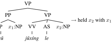
[image:3.612.314.547.65.413.2]→heldx2withx1
Figure 2: Tree-to-string ruler3for reordering.
2.2 Beam Search in Practice
To make the exponential algorithm practical, beam search is the standard approximate search method (Koehn, 2004). Here we group +LM items inton
bins, with each binBi hosting at most bitems that cover exactly iChinese words (see Figure 1). The complexity becomesO(n2b)because there are a to-tal of O(nb) items in all bins, and to expand each item we need to scan the whole coverage vector, which costsO(n). This quadratic complexity is still too slow in practice and we often set a small
distor-tion limit of dmax (say, 5) so that no jumps longer than dmax are allowed. This method reduces the complexity toO(nbdmax)but fails to capture long-distance reorderings (Galley and Manning, 2008).
3 Incremental Decoding for Tree-to-String Translation
We will first briefly review tree-to-string translation paradigm and then develop an incremental decoding algorithm for it inspired by phrase-based decoding.
3.1 Tree-to-string Translation
A typical tree-to-string system (Liu et al., 2006; Huang et al., 2006) performs translation in two steps: parsing and decoding. A parser first parses the source language input into a 1-best treeT, and the decoder then searches for the best derivation (a
se-(a) B`ush´ı [yˇu Sh¯al´ong ]1 [jˇux´ıng le hu`ıt´an ]2
⇓1-best parser
(b) IP@ǫ
NP@1
B`ush´ı
VP@2
P
yˇu
Sh¯al´ong
VV
jˇux´ıng
AS
le
hu`ıt´an
r1 ⇓ (c) NP@1
B`ush´ı
VP@2
P
yˇu
Sh¯al´ong
VV
jˇux´ıng
AS
le
hu`ıt´an
r2⇓ r3 ⇓ (d) Bush held NP@2.2.3
hu`ıt´an
with NP@2.1.2
Sh¯al´ong
r4⇓ r5 ⇓
(e) Bush [held talks]2 [with Sharon]1
Figure 3: An example derivation of tree-to-string trans-lation (much simplified from Mi et al. (2008)). Shaded regions denote parts of the tree that matches the rule.
quence of translation steps)d∗ that converts source treeT into a target-language string.
Figure 3 shows how this process works. The Chi-nese sentence (a) is first parsed into tree (b), which will be converted into an English string in 5 steps. First, at the root node, we apply ruler1 preserving the top-level word-order
(r1) IP (x1:NP x2:VP)→x1 x2
which results in two unfinished subtrees, NP@1and VP@2 in (c). HereX@η denotes a tree node of
la-belX at tree addressη (Shieber et al., 1995). (The root node has addressǫ, and the first child of nodeη
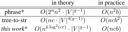
[image:3.612.77.296.191.274.2]in theory in practice phrase* O(2nn2· |V|g−1) O(n2b) tree-to-str O(nc· |V|4(g−1)
) O(ncb2)
this work* O(nklog2(cr)
[image:4.612.76.297.57.113.2]· |V|g−1) O(ncb)
Table 2: Summary of time complexities of various algo-rithms.bis the beam width,V is the English vocabulary, andc is the number of translation rules per node. As a special case, phrase-based decoding with distortion limit dmaxisO(nbdmax). *: incremental decoding algorithms.
“Bush”. Similarly, ruler3 shown in Figure 2 is ap-plied to the VP subtree, which swaps the two NPs, yielding the situation in (d). Finally two phrasal rulesr4 andr5 translate the two remaining NPs and finish the translation.
In this framework, decoding without language model (−LM decoding) is simply a linear-time depth-first search with memoization (Huang et al., 2006), since a tree of n words is also of size
O(n) and we visit every node only once. Adding a language model, however, slows it down signifi-cantly because we now have to keep track of target-language boundary words, but unlike the phrase-based case in Section 2, here we have to remember both sides the leftmost and the rightmost boundary words: each node is now split into+LM items like
(ηa⋆b)whereηis a tree node, andaandbare left
and right English boundary words. For example, a bigram+LM item for node VP@2might be
(VP@2held⋆Sharon).
This is also the case with other syntax-based models like Hiero or GHKM: language model integration overhead is the most significant factor that causes syntax-based decoding to be slow (Chiang, 2007). In theory+LM decoding isO(nc|V|4(g−1)
), whereV
denotes English vocabulary (Huang, 2007). In prac-tice we have to resort to beam search again: at each node we would only allow top-b+LM items. With beam search, tree-to-string decoding with an inte-grated language model runs in timeO(ncb2), where
bis the size of the beam at each node, andcis (max-imum) number of translation rules matched at each node (Huang, 2007). See Table 2 for a summary.
3.2 Incremental Decoding
Can we borrow the idea of phrase-based decoding, so that we also grow the hypothesis strictly left-to-right, and only need to maintain the rightmost boundary words?
The key intuition is to adapt the coverage-vector idea from phrase-based decoding to tree-to-string decoding. Basically, a coverage-vector keeps track of which Chinese spans have already been translated and which have not. Similarly, here we might need a “tree coverage-vector” that indicates which sub-trees have already been translated and which have not. But unlike in phrase-based decoding, we can not simply choose any arbitrary uncovered subtree for the next step, since rules already dictate which subtree to visit next. In other words what we need here is not really a tree coverage vector, but more of a derivation history.
We develop this intuition into an agenda repre-sented as a stack. Since tree-to-string decoding is a top-down depth-first search, we can simulate this re-cursion with a stack of active rules, i.e., rules that are not completed yet. For example we can simulate the derivation in Figure 3 as follows. At the root node IP@ǫ, we choose rule r1, and push its English-side to the stack, with variables replaced by matched tree nodes, here x1 for NP@1 and x2 for VP@2. So we have the following stack
s=[NP@1VP@2],
where the dotindicates the next symbol to process in the English word-order. Since node NP@1 is the first in the English word-order, we expand it first, and push ruler2 rooted at NP to the stack:
[NP@1VP@2] [Bush].
Since the symbol right after the dot in the top rule is a word, we immediately grab it, and append it to the current hypothesis, which results in the new stack
[NP@1VP@2] [Bush].
Now the top rule on the stack has finished (dot is at the end), so we trigger a “pop” operation which pops the top rule and advances the dot in the second-to-top rule, denoting that NP@1is now completed:
stack hypothesis
[<s>IP@ǫ</s>] <s>
[image:5.612.74.553.81.298.2]p [<s>IP@ǫ</s>] [NP@1VP@2] <s> p [<s>IP@ǫ</s>] [NP@1VP@2] [Bush] <s> s [<s>IP@ǫ</s>] [NP@1VP@2] [Bush] <s>Bush c [<s>IP@ǫ</s>] [NP@1VP@2] <s>Bush p [<s>IP@ǫ</s>] [NP@1VP@2] [held [email protected] [email protected]] <s>Bush s [<s>IP@ǫ</s>] [NP@1VP@2] [held[email protected] [email protected]] <s>Bush held p [<s>IP@ǫ</s>] [NP@1VP@2] [held[email protected] [email protected]] [talks] <s>Bush held s [<s>IP@ǫ</s>] [NP@1VP@2] [held[email protected] [email protected]] [talks] <s>Bush held talks c [<s>IP@ǫ</s>] [NP@1VP@2] [held [email protected]with [email protected]] <s>Bush held talks s [<s>IP@ǫ</s>] [NP@1VP@2] [held [email protected][email protected]] <s>Bush held talks with p [<s>IP@ǫ</s>] [NP@1VP@2] [held [email protected][email protected]] [Sharon] <s>Bush held talks with s [<s>IP@ǫ</s>] [NP@1VP@2] [held [email protected][email protected]] [Sharon] <s>Bush held talks with Sharon c [<s>IP@ǫ</s>] [NP@1VP@2] [held [email protected] [email protected]] <s>Bush held talks with Sharon c [<s>IP@ǫ</s>] [NP@1VP@2] <s>Bush held talks with Sharon c [<s>IP@ǫ</s>] <s>Bush held talks with Sharon s [<s>IP@ǫ</s>] <s>Bush held talks with Sharon</s>
Figure 4: Simulation of tree-to-string derivation in Figure 3 in the incremental decoding algorithm. Actions:p, predict; s, scan;c, complete (see Figure 5).
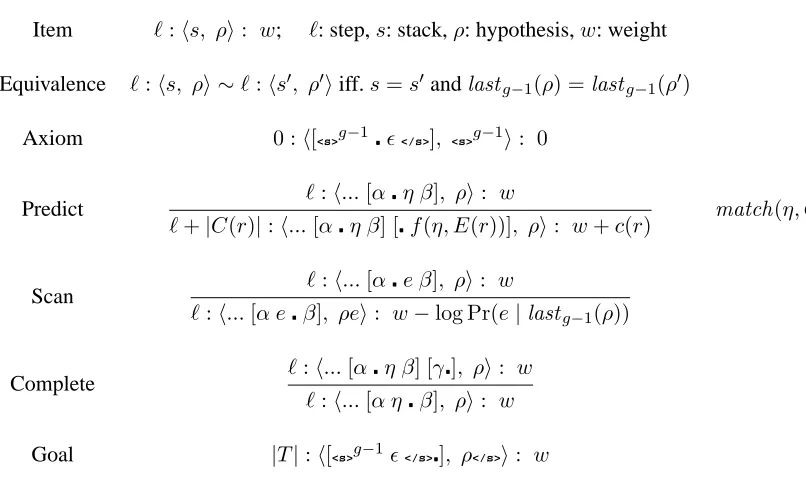
Item ℓ:hs, ρi: w; ℓ: step,s: stack,ρ: hypothesis,w: weight
Equivalence ℓ:hs, ρi ∼ℓ:hs′, ρ′iiff.s=s′ andlastg−1(ρ) =lastg−1(ρ′)
Axiom 0 :h[<s>g−1ǫ</s>], <s>g−1i: 0
Predict ℓ:h...[αη β], ρi: w
ℓ+|C(r)|:h...[αη β] [f(η, E(r))], ρi: w+c(r) match(η, C(r))
Scan ℓ:h...[αe β], ρi: w
ℓ:h...[α eβ], ρei: w−log Pr(e|lastg−1(ρ))
Complete ℓ:h...[αη β] [γ], ρi: w
ℓ:h...[α ηβ], ρi: w
Goal |T|:h[<s>g−1ǫ</s>], ρ</s>i: w
Figure 5: Deductive system for the incremental tree-to-string decoding algorithm. Function lastg−1(·) returns the rightmostg−1 words (forg-gram LM), andmatch(η, C(r))tests matching of ruleragainst the subtree rooted at nodeη.C(r)andE(r)are the Chinese and English sides of ruler, and functionf(η, E(r)) = [xi7→η.var(i)]E(r)
[image:5.612.92.495.375.620.2]The next step is to expand VP@2, and we use ruler3 and push its English-side “VP→heldx2withx1” onto the stack, again with variables replaced by matched nodes:
[NP@1VP@2] [held [email protected] [email protected]]
Note that this is a reordering rule, and the stack al-ways follows the English word order because we generate hypothesis incrementally left-to-right. Fig-ure 4 works out the full example.
We formalize this algorithm in Figure 5. Each item hs, ρi consists of a stack s and a hypothesis
ρ. Similar to phrase-based dynamic programming, only the lastg−1words ofρare part of the signature for decoding withg-gram LM. Each stack is a list of
dotted rules, i.e., rules with dot positions indicting
progress, in the style of Earley (1970). We call the last (rightmost) rule on the stack the top rule, which is the rule being processed currently. The symbol af-ter the dot in the top rule is called the next symbol, since it is the symbol to expand or process next. De-pending on the next symbola, we can perform one of the three actions:
• if ais a node η, we perform a Predict action which expandsηusing a rulerthat can pattern-match the subtree rooted atη; we pushr is to the stack, with the dot at the beginning;
• ifais an English word, we perform a Scan ac-tion which immediately adds it to the current hypothesis, advancing the dot by one position;
• if the dot is at the end of the top rule, we perform a Complete action which simply pops stack and advance the dot in the new top rule.
3.3 Polynomial Time Complexity
Unlike phrase-based models, we show here that incremental decoding runs in average-case polynomial-time for tree-to-string systems.
Lemma 1. For an input sentence of n words and its parse tree of depth d, the worst-case complex-ity of our algorithm is f(n, d) = c(cr)d|V|g−1
=
O((cr)dng−1), assuming relevant English
vocabu-lary|V|=O(n), and where constantsc,randgare the maximum number of rules matching each tree node, the maximum arity of a rule, and the language-model order, respectively.
Proof. The time complexity depends (in part) on the
number of all possible stacks for a tree of depthd. A stack is a list of rules covering a path from the root node to one of the leaf nodes in the following form:
R1
z }| {
[...η1...] R2
z }| {
[...η2...]... Rs
z }| {
[...ηs...],
whereη1 =ǫis the root node andηsis a leaf node,
with stack depth s ≤ d. Each rule Ri(i > 1)
ex-pands nodeηi−1, and thus hascchoices by the defi-nition of grammar constantc. Furthermore, each rule in the stack is actually a dotted-rule, i.e., it is associ-ated with a dot position ranging from 0 tor, wherer
is the arity of the rule (length of English side of the rule). So the total number of stacks isO((cr)d).
Besides the stack, each state also maintains(g−1)
rightmost words of the hypothesis as the language model signature, which amounts to O(|V|g−1). So the total number of states isO((cr)d|V|g−1). Fol-lowing previous work (Chiang, 2007), we assume a constant number of English translations for each foreign word in the input sentence, so|V|=O(n). And as mentioned above, for each state, there arec
possible expansions, so the overall time complexity isf(n, d) =c(cr)d|V|g−1 =O((cr)dng−1).
We do average-case analysis below because the tree depth (height) for a sentence of n words is a random variable: in the worst-case it can be linear in
n(degenerated into a linear-chain), but we assume this adversarial situation does not happen frequently, and the average tree depth isO(logn).
Theorem 1. Assume for each n, the depth of a parse tree of n words, notated dn, distributes
nor-mally with logarithmic mean and variance, i.e.,
dn ∼ N(µn, σ2n), where µn = O(logn)andσ2n =
O(logn), then the average-case complexity of the algorithm ish(n) =O(nklog2(cr)+g−1)for constant k, thus polynomial inn.
Proof. From Lemma 1 and the definition of
average-case complexity, we have
h(n) =Edn∼N(µn,σn2)[f(n, dn)],
to the random variablexin distributionD.
h(n) = Edn∼N(µn,σn2)[f(n, dn)]
= Edn∼N(µn,σn2)[O((cr)
dnng−1)],
= O(ng−1Edn∼N(µn,σ2n)[(cr) dn
]),
= O(ng−1Edn∼N(µn,σ2n)[exp(dnlog(cr))]) (2)
Since dn ∼ N(µn, σn2) is a normal distribution,
dnlog(cr) ∼ N(µ′, σ′2) is also a normal distribu-tion, whereµ′ = µnlog(cr) andσ′ = σnlog(cr). Thereforeexp(dnlog(cr))is a log-normal distribu-tion, and by the property of log-normal distribudistribu-tion, its expectation isexp (µ′+σ′2/2). So we have
Edn∼N(µn,σ2/2)[exp(dnlog(cr))]
= exp (µ′+σ′2/2)
= exp (µnlog(cr) +σ2nlog2(cr)/2)
= exp (O(logn) log(cr) +O(logn) log2(cr)/2) = exp (O(logn) log2(cr))
≤ exp (k(logn) log2(cr)), for some constantk
= exp (lognklog2(cr)
)
= nklog2(cr). (3)
Plug it back to Equation (2), and we have the average-case complexity
Edn[f(n, dn)] ≤ O(n
g−1nklog2(cr)
)
= O(nklog2(cr)+g−1). (4)
Since k,c,r andgare constants, the average-case complexity is polynomial in sentence lengthn.
The assumption dn ∼ N(O(logn), O(logn))
will be empirically verified in Section 5.
3.4 Linear-time Beam Search
Though polynomial complexity is a desirable prop-erty in theory, the degree of the polynomial,
O(logcr)might still be too high in practice, depend-ing on the translation grammar. To make it linear-time, we apply the beam search idea from phrase-based again. And once again, the only question to decide is the choice of “binning”: how to assign each item to a particular bin, depending on their progress? While the number of Chinese words covered is a natural progress indicator for phrase-based, it does not work for tree-to-string because, among the three actions, only scanning grows the hypothesis. The prediction and completion actions do not make real
progress in terms of words, though they do make progress on the tree. So we devise a novel progress indicator natural for tree-to-string translation: the number of tree nodes covered so far. Initially that number is zero, and in a prediction step which ex-pands nodeηusing ruler, the number increments by
|C(r)|, the size of the Chinese-side treelet ofr. For example, a prediction step using ruler3 in Figure 2 to expand VP@2will increase the tree-node count by
|C(r3)| = 6, since there are six tree nodes in that rule (not counting leaf nodes or variables).
Scanning and completion do not make progress in this definition since there is no new tree node covered. In fact, since both of them are determin-istic operations, they are treated as “closure” op-erators in the real implementation, which means that after a prediction, we always do as many scan-ning/completion steps as possible until the symbol after the dot is another node, where we have to wait for the next prediction step.
This method has|T| = O(n) bins where|T|is the size of the parse tree, and each bin holdsbitems. Each item can expand tocnew items, so the overall complexity of this beam search isO(ncb), which is linear in sentence length.
4 Related Work
The work of Watanabe et al. (2006) is closest in spirit to ours: they also design an incremental decod-ing algorithm, but for the hierarchical phrase-based system (Chiang, 2007) instead. While we leave de-tailed comparison and theoretical analysis to a future work, here we point out some obvious differences:
1. due to the difference in the underlying trans-lation models, their algorithm runs inO(n2b) time with beam search in practice while ours is linear. This is because each prediction step now hasO(n) choices, since they need to ex-pand nodes like VP[1, 6] as:
VP[1,6]→PP[1,i] VP[i, 6],
where the midpoint i in general has O(n)
choices (just like in CKY). In other words, their grammar constantcbecomesO(n).
orig-inal phrase-based idea of number of Chinese words translated;
3. as a result, their framework requires gram-mar transformation into the binary-branching Greibach Normal Form (which is not always possible) so that the resulting grammar always contain at least one Chinese word in each rule in order for a prediction step to always make progress. Our framework, by contrast, works with any grammar.
Besides, there are some other efforts less closely related to ours. As mentioned in Section 1, while we focus on enhancing syntax-based decoding with phrase-based ideas, other authors have explored the reverse, but also interesting, direction of enhancing phrase-based decoding with syntax-aware reorder-ing. For example Galley and Manning (2008) pro-pose a shift-reduce style method to allow hiearar-chical non-local reorderings in a phrase-based de-coder. While this approach is certainly better than pure phrase-based reordering, it remains quadratic in run-time with beam search.
Within syntax-based paradigms, cube pruning (Chiang, 2007; Huang and Chiang, 2007) has be-come the standard method to speed up +LM de-coding, which has been shown by many authors to be highly effective; we will be comparing our incre-mental decoder with a baseline decoder using cube pruning in Section 5. It is also important to note that cube pruning and incremental decoding are not mutually exclusive, rather, they could potentially be combined to further speed up decoding. We leave this point to future work.
Multipass coarse-to-fine decoding is another pop-ular idea (Venugopal et al., 2007; Zhang and Gildea, 2008; Dyer and Resnik, 2010). In particular, Dyer and Resnik (2010) uses a two-pass approach, where their first-pass, −LM decoding is also incremental and polynomial-time (in the style of Earley (1970) algorithm), but their second-pass,+LM decoding is still bottom-up CKY with cube pruning.
5 Experiments
To test the merits of our incremental decoder we conduct large-scale experiments on a state-of-the-art tree-to-string system, and compare it with the stan-dard phrase-based system of Moses. Furturemore we
also compare our incremental decoder with the stan-dard cube pruning approach on the same tree-to-string decoder.
5.1 Data and System Preparation
Our training corpus consists of 1.5M sentence pairs with about 38M/32M words in Chinese/English, re-spectively. We first word-align them by GIZA++ and then parse the Chinese sentences using the Berke-ley parser (Petrov and Klein, 2007), then apply the GHKM algorithm (Galley et al., 2004) to ex-tract tree-to-string translation rules. We use SRILM Toolkit (Stolcke, 2002) to train a trigram language model with modified Kneser-Ney smoothing on the target side of training corpus. At decoding time, we again parse the input sentences into trees, and convert them into translation forest by rule pattern-matching (Mi et al., 2008).
We use the newswire portion of 2006 NIST MT Evaluation test set (616 sentences) as our develop-ment set and the newswire portion of 2008 NIST MT Evaluation test set (691 sentences) as our test set. We evaluate the translation quality using the BLEU-4 metric, which is calculated by the script mteval-v13a.pl with its default setting which is case-insensitive matching of n-grams. We use the stan-dard minimum error-rate training (Och, 2003) to tune the feature weights to maximize the system’s BLEU score on development set.
We first verify the assumptions we made in Sec-tion 3.3 in order to prove the theorem that tree depth (as a random variable) is normally-distributed with
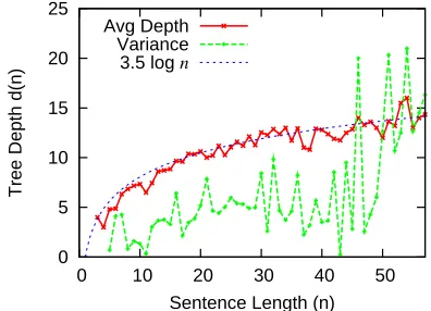
O(logn)mean and variance. Qualitatively, we veri-fied that for mostn, tree depthd(n)does look like a normal distribution. Quantitatively, Figure 6 shows that average tree height correlates extremely well with3.5 logn, while tree height variance is bounded by5.5 logn.
5.2 Comparison with Cube pruning
We implemented our incremental decoding algo-rithm in Python, and test its performance on the de-velopment set. We first compare it with the stan-dard cube pruning approach (also implemented in Python) on the same tree-to-string system.1
Fig-1Our implementation of cube pruning follows (Chiang,
2007; Huang and Chiang, 2007) where besides a beam sizeb
0 1 2 3 4 5
0 10 20 30 40 50 60 70
Average Decoding Time (Secs)
Sentence Length incremental
cube pruning
29.5 29.6 29.7 29.8 29.9 30 30.1
0 0.2 0.4 0.6 0.8 1 1.2 1.4
BLEU Score
Avg Decoding Time (secs per sentence) incremental
cube pruning
[image:9.612.93.509.58.218.2](a) decoding time against sentence length (b) BLEU score against decoding time
Figure 7: Comparison with cube pruning. The scatter plot in (a) confirms that our incremental decoding scales linearly with sentence length, while cube pruning super-linearly (b = 50for both). The comparison in (b) shows that at the same level of translation quality, incremental decoding is slightly faster than cube pruning, especially at smaller beams.
0 5 10 15 20 25
0 10 20 30 40 50
Tree Depth d(n)
Sentence Length (n) Avg Depth
Variance 3.5 log n
Figure 6: Mean and variance of tree depth vs. sentence length. The mean depth clearly scales with3.5 logn, and the variance is bounded by5.5 logn.
ure 7(a) is a scatter plot of decoding times versus sentence length (using beam b = 50 for both sys-tems), where we confirm that our incremental de-coder scales linearly, while cube pruning has a slight tendency of superlinearity. Figure 7(b) is a side-by-side comparison of decoding speed versus transla-tion quality (in BLEU scores), using various beam sizes for both systems (b=10–70 for cube pruning, andb=10–110 for incremental). We can see that in-cremental decoding is slightly faster than cube prun-ing at the same levels of translation quality, and the difference is more pronounced at smaller beams: for
number of (non-unique) pops from priority queues.
0 5 10 15 20 25 30 35 40
0 10 20 30 40 50 60 70
Average Decoding Time (Secs)
Sentence Length M +∞
[image:9.612.79.277.304.447.2]M 10 M 6 M 0 t2s
Figure 8: Comparison of our incremental tree-to-string decoder with Moses in terms of speed. Moses is shown with various distortion limits (0, 6, 10,+∞; optimal: 10).
example, at the lowest levels of translation quality (BLEU scores around 29.5), incremental decoding takes only 0.12 seconds, which is about 4 times as fast as cube pruning. We stress again that cube prun-ing and incremental decodprun-ing are not mutually ex-clusive, and rather they could potentially be com-bined to further speed up decoding.
5.3 Comparison with Moses
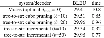
[image:9.612.320.518.304.447.2]system/decoder BLEU time Moses (optimaldmax=10) 29.41 10.8 tree-to-str: cube pruning (b=10) 29.51 0.65 tree-to-str: cube pruning (b=20) 29.96 0.96 tree-to-str: incremental (b=10) 29.54 0.32 tree-to-str: incremental (b=50) 29.96 0.77
Table 3: Final BLEU score and speed results on the test data (691 sentences), compared with Moses and cube pruning. Time is in seconds per sentence, including pars-ing time (0.21s) for the two tree-to-strpars-ing decoders.
with Moses at various distortion limits (dmax=0, 6, 10, and +∞). Consistent with the theoretical anal-ysis in Section 2, Moses with no distortion limit (dmax = +∞) scale quadratically, and monotone decoding (dmax = 0) scale linearly. We use MERT to tune the best weights for each distortion limit, and
dmax= 10performs the best on our dev set.
Table 3 reports the final results in terms of BLEU score and speed on the test set. Our linear-time incremental decoder with the small beam of size
b = 10 achieves a BLEU score of 29.54, compara-ble to Moses with the optimal distortion limit of 10 (BLEU score 29.41). But our decoding (including source-language parsing) only takes 0.32 seconds a sentences, which is more than 30 times faster than Moses. With a larger beam of b = 50our BLEU score increases to 29.96, which is a half BLEU point better than Moses, but still about 15 times faster.
6 Conclusion
We have presented an incremental dynamic pro-gramming algorithm for tree-to-string translation which resembles phrase-based based decoding. This algorithm is the first incremental algorithm that runs in polynomial-time in theory, and linear-time in practice with beam search. Large-scale experiments on a state-of-the-art tree-to-string decoder confirmed that, with a comparable (or better) translation qual-ity, it can run more than 30 times faster than the phrase-based system of Moses, even though ours is in Python while Moses in C++. We also showed that it is slightly faster (and scale better) than the popular cube pruning technique. For future work we would like to apply this algorithm to forest-based transla-tion and hierarchical system by pruning the first-pass
−LM forest. We would also combine cube pruning
with our incremental algorithm, and study its perfor-mance with higher-order language models.
Acknowledgements
We would like to thank David Chiang, Kevin Knight, and Jonanthan Graehl for discussions and the anonymous reviewers for comments. In partic-ular, we are indebted to the reviewer who pointed out a crucial mistake in Theorem 1 and its proof in the submission. This research was supported in part by DARPA, under contract HR0011-06-C-0022 under subcontract to BBN Technologies, and under DOI-NBC Grant N10AP20031, and in part by the National Natural Science Foundation of China, Con-tracts 60736014 and 90920004.
References
David Chiang. 2007. Hierarchical phrase-based transla-tion. Computational Linguistics, 33(2):201–208. Chris Dyer and Philip Resnik. 2010. Context-free
re-ordering, finite-state translation. In Proceedings of NAACL.
Jay Earley. 1970. An efficient context-free parsing algo-rithm. Communications of the ACM, 13(2):94–102. Michel Galley and Christopher D. Manning. 2008. A
simple and effective hierarchical phrase reordering model. In Proceedings of EMNLP 2008.
Michel Galley, Mark Hopkins, Kevin Knight, and Daniel Marcu. 2004. What’s in a translation rule? In Pro-ceedings of HLT-NAACL, pages 273–280.
Liang Huang and David Chiang. 2007. Forest rescor-ing: Fast decoding with integrated language models. In Proceedings of ACL, Prague, Czech Rep., June. Liang Huang, Kevin Knight, and Aravind Joshi. 2006.
Statistical syntax-directed translation with extended domain of locality. In Proceedings of AMTA, Boston, MA, August.
Liang Huang. 2007. Binarization, synchronous bina-rization, and target-side binarization. In Proc. NAACL Workshop on Syntax and Structure in Statistical Trans-lation.
Kevin Knight. 1999. Decoding complexity in word-replacement translation models. Computational Lin-guistics, 25(4):607–615.
Philipp Koehn. 2004. Pharaoh: a beam search decoder for phrase-based statistical machine translation mod-els. In Proceedings of AMTA, pages 115–124. Yang Liu, Qun Liu, and Shouxun Lin. 2006.
Tree-to-string alignment template for statistical machine trans-lation. In Proceedings of COLING-ACL, pages 609– 616.
Haitao Mi, Liang Huang, and Qun Liu. 2008. Forest-based translation. In Proceedings of ACL: HLT, Columbus, OH.
Franz Joseph Och. 2003. Minimum error rate training in statistical machine translation. In Proceedings of ACL, pages 160–167.
Slav Petrov and Dan Klein. 2007. Improved inference for unlexicalized parsing. In Proceedings of HLT-NAACL.
Stuart Shieber, Yves Schabes, and Fernando Pereira. 1995. Principles and implementation of deductive parsing. Journal of Logic Programming, 24:3–36. Andreas Stolcke. 2002. Srilm - an extensible
lan-guage modeling toolkit. In Proceedings of ICSLP, vol-ume 30, pages 901–904.
Ashish Venugopal, Andreas Zollmann, and Stephen Vo-gel. 2007. An efficient two-pass approach to synchronous-CFG driven statistical MT. In Proceed-ings of HLT-NAACL.
Taro Watanabe, Hajime Tsukuda, and Hideki Isozaki. 2006. Left-to-right target generation for hierarchical phrase-based translation. In Proceedings of COLING-ACL.
Dekai Wu. 1997. Stochastic inversion transduction grammars and bilingual parsing of parallel corpora. Computational Linguistics, 23(3):377–404.