A thermal electrical analogy model of a four floor building with occupancy estimation for heating system control

A thermal–electrical analogy model of a

four–floor building with occupancy

estimation for heating system control

?

O. Tate∗D. Cheneler∗C. J. Taylor∗

∗_{Engineering Department, Lancaster University, UK}

(e-mail: [email protected], [email protected], [email protected])

Abstract:The well-known electrical analogy for thermal modelling is based on the observation that Fourier’s equation for one dimensional heat transfer takes the same form as Ohm’s law. This provides a system for creating and resolving complex heat transfer problems using an established set of physically–based equations. In this article, such a model is developed and evaluated for a four–floor modern university building. The model is represented in state space form for optimisation and simulation purposes. The electrical analogy is chosen so that the model can be extended and used for future research into distributed, demand–side control of multiple buildings on the university network, requiring a fast computation time. The estimation of occupancy, representing a significant internal heat source, is also investigated. Here, wifi usage and return CO2 data are combined in novel manner to improve the model response.

Keywords:thermal modelling; buildings occupancy; micro-climate; state space model.

1. INTRODUCTION

The research behind this article ultimately concerns con-trol system robustness and overall system optimisation, for the regulation of temperatures in buildings that are linked to a controllable external heating supply network. This is the case, for example, with the Lancaster University campus, for which a central energy centre supplies the hot water used to heat around 50% of the buildings. More gen-erally, Heating, Ventilation and Air Conditioning (HVAC) systems have high energy requirements, hence there is considerable interest in the development of improved op-timisation tools, micro–climate control algorithms and en-ergy management systems. Examples include Price et al. (1999); Taylor et al. (2004); Yang and Wang (2013); Kim (2013); Goyal et al. (2013); Kossak and Stadler (2015); Uribe et al. (2015); Mayer et al. (2017); Gorni and Visioli (2017); Zhuang et al. (2018); Tate et al. (2018).

Numerous approaches for modelling heat transfer phe-nomena and energy use have been developed. The models obtained are commonly categorised into physically–based models and models that are statistically identified from data (Foucquier et al., 2013). Within this context, various zonal and multi–zone approaches exist. Of particular rele-vance to the present article, these include thermal models constructed using an analogy with electrical systems. This is based on the observation that Fourier’s equation for one dimensional heat transfer takes the same form as Ohm’s law. An early reference by Paschkis and Baker (1942) describes how components of a building are considered to store or resist heat flows, equivalent to capacitors and re-sistors in electrical systems (Ramirez-Laboreo et al., 2014). ? _{This work is supported by Engineering and Physical Sciences}

Research Council (EPSRC): EP/M015637/1.

This is useful as it provides a system for creating and resolving heat transfer problems using an established set of physically–based laws. Whilst page constraints preclude a full literature review here, relevant research includes e.g. multiple layered walls (Peng and Wu, 2008), heat exchanger networks (Chen et al., 2015), global building models (Fraisse et al., 2002), parameter estimation, opti-mal model order identification and model reduction (Pen-man, 1990; Gouda et al., 2002; Goyal and Barooah, 2012). Relatively high order resistor–capacitor (RC) networks are sometimes employed in order to model building compo-nents. For example, Peng and Wu (2008) represent a wall consisting of multiple layers of materials with air gaps, as a system with three resistors and one capacitor (denoted 3R1C). However, as a greater number of zones are mod-elled concurrently, the network diagrams can become very large. In such cases, programs such as TRNSYS (Klein et al., 1978) are used to collate the models.

Analysis of the initial model highlights a limitation, namely the lack of a suitable internal heat source to represent changing occupancy rates. The rooms are office spaces, hence human occupancy and electrical equipment will contribute heat (Luo et al., 2018; Tabak and de Vries, 2010; Yang and Becerik-Gerber, 2014). As a result, the model is extended to include occupancy estimated using data on (floor by floor) wifi usage and CO2 levels

(asso-ciated with each of the air handling units) in the Charles Carter Building. The new model is expressed in state– space form and evaluated at full building scale.

2. CASE STUDY

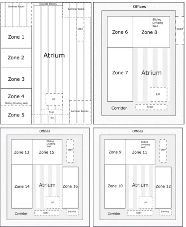
Lancaster University campus has several recently con-structed buildings fully instrumented with a range of sen-sors and actuators, and seems well suited for research into the optimisation of energy efficiency because of the associated BMS data collection capacity. The architects of the Charles Carter Building, for example, integrated various energy–reducing features into the building design, which achieved a BREEAM Excellent rating. The south elevation is designed to shade the building while the con-crete roof protects the top floor from heating up in the sun. The building footprint is 33 m by 36 m, while there are four floors (A–D), as illustrated by Fig. 1. Internally the building is laid out around a central atrium that is open from the floor to the roof. Surrounding this area are lecture theatres, offices, meeting rooms and break-out spaces.

Micro-climate data are collected by the BMS every 10 minutes including, for example, the supply and return air temperatures for various rooms, ventilation power levels and HVAC set points. For purpose of the present article, the main occupied rooms are represented as 16 zones in Fig. 1, each representing an individual Air Handling Unit (AHU) with measured ‘return’ air temperatureTi(t)

(i= 1, . . . ,16). Illustrative temperature measurements are shown for two such zones in Fig. 2 (degrees Celsius,◦C).

3. MODEL FORMULATION

The model is expressed in conventional continuous-time state space form, as follows,

˙

x(t) =Ax(t) +Bu(t)

y(t) =Cx(t) +Du(t) (1)

where y(t) is a 16×1 vector of output variables, i.e. the temperature Ti(t) in each zone and u(t) is a 34×1

vector of input variables, with elementsui(t) (section 3.1).

In the physically–based model developed below, C is an identity matrix andD=0is a matrix of zeros, hence the state vector x(t) = y(t). Finally, A and B are matrices with elementsaij (i, j= 1, . . . ,16) andbij (i= 1, . . . ,16,

j= 1, . . . ,34) respectively (see sections 3.2 and 3.3).

3.1 Heat inputs

The total heat input to each zone, qi(t) (i = 1, . . . ,16)

(W), consists of three components as follows,

qi(t) =i(t) +γi(t) +ζi(t) (2)

wherei(t) =hicap m˙i(t)δTi(t) is the controlled heat flow

from the AHU (either cooling or heating), γi(t) = (ω+

σi)gi(t) is an internal heat source andζi(t) =φiM(t) is the

heat supplied from the campus hot water heating system.

Here, ca

p is the the specific heat capacity of air; ˙mi(t) is

the mass flow of the air handling unit in zonei(m3 _s−1_);

δTi(t) =Si(t)−Ti(t) is the temperature difference between

the supply and return air, in which Si(t) is the inlet air

temperature; andhi= 0.9 ∀i(initial assumption, prior to

optimisation) is an empirical mixing coefficient, introduced since not all of the incoming air mass will be fully mixed before it is extracted at the outlet. The mass flow is not directly measured and so is determined as follows,

˙

mi(t) =f ρari(t) (3)

where f = 0.006 m6 kg−1 is a fan properties coefficient, representing the effective diameter and pitch, ρa is the

air density and ri(t) represents the fan RPM/60 i.e.

revolutions per second. Hence,i(t) = hi cpa f ρa·ri(t)·

δTi(t), which is bilinear inri(t) andδTi(t), and a function

of the zone temperature, raising identifiability challenges that are the subject of current research by the authors.

With regard to the internal heat source, gi(t) represents

the time–varying number of occupants in each room, while ω = 100 W is based on an assumed average heat output per person (Luo et al., 2018). The additional heat gain coefficients σi = 10 W for i = 1, . . . ,5 and σi = 50 W

fori= 6, . . . ,16 are associated with electronic equipment. These initial values (prior to optimisation) are based on an assumption that Floor A is primarily used for teaching, whilst on floors B–D staff utilise desktop computers.

In ζi(t), M(t) represents the heat supplied by hot water

entering the building from the campus-wide heating sys-tem (W), while the proportion of this heat that reaches a particular zone is denotedφi. There are a number of data

collection limitations associated with these terms, hence they are the subject of on-going research. For the purpose of the present article, 50% of the heat is assumed to reach the modelled zones, andφi is initially assumed to be split

equally between these zones, henceφi= 0.03∀i(retaining

the index since this coefficient can potentially be optimised from data for each zonei).

To represent these heat inputs via equations (1), the first sixteen elements of u(t) are defined ui(t) = gi(t)

(i = 1, . . . ,16), i.e. the number of occupants; and the next sixteen elements,uj(t) =ri(t)δTi(t) (j= 17, . . . ,32;

i = 1, . . . ,16) are the input signals associated with the controlled heat flow from each AHU. Finally, u34(t) =

M(t), while u33(t) = TE(t) is an additional exogenous

variable, namely the outdoor temperature. The various time–invariant coefficients alluded to above are embedded inAandB, defined from first principles or estimated from data, as discussed below.

3.2 Heat balance equations

Fig. 1. Floor layouts showing zone numbers corresponding to model states: clockwise from top left, floor A, B, C and D.

Fri Sat Sun Mon Tue Wed Thu 20

22 24

oC room 2

room 1

Fri Sat Sun Mon Tue Wed Thu 15

20 25 30

oC

supply 2 supply 1

Fri Sat Sun Mon Tue Wed Thu day of the week

10 20

oC

ambient outside

Fig. 2. Illustrative room (return) and supply (air condi-tioning) temperatures, Friday 1st to 7th Sept. 2017.

consider the temperature T2(t) for zone 2 on A–floor.

The temperature in this zone is coupled to the adjacent zones 1 and 3, with temperatures T1(t) and T3(t), and

T6(t) above on B–floor. Hence, assuming heat capacityC2

and walls/floors of thermal resistanceR1,2,R2,3,R2,6and

R2,E, standard heat balance equations yield,

q2(t) =C2

dT2(t)

dt +

T2(t)−T1(t)

R1,2

+T2(t)−T3(t) R2,3

+T2(t)−T6(t) R2,6

+T2(t)−TE(t) R2,E

(4)

in which q2(t) represents the total heat flow (2).

Re-arranging to isolate the relevant state yields,

dT2(t)

dt =

q2(t)

C2

+ T1(t) C2R1,2

+ T3(t) C2R2,3

+ T6(t) C2R2,6

+ TE(t) C2R2,E

−T2(t) C2

₁

R1,2

+ 1

R2,3

+ 1

R2,6

+ 1

R2,E

Noting that u2(t) = g2(t) and u18(t) = r2(t)δT2(t),

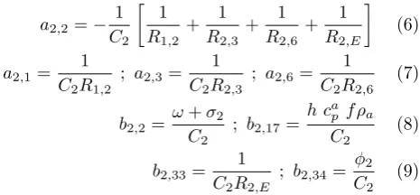
equation (5) is represented in the state space model (1), by defining the following elements forAandB,

a2,2=−

1 C2

₁

R1,2

+ 1

R2,3

+ 1

R2,6

+ 1

R2,E

(6)

a2,1=

1 C2R1,2

; a2,3=

1 C2R2,3

; a2,6=

1 C2R2,6

(7)

b2,2=

ω+σ2

C2

; b2,17=

h cap f ρa

C2

(8)

b2,33=

1 C2R2,E

; b2,34=

φ2

C2

(9)

The remaining elements on the second row ofAandBare zero. Similar 1R1C models are developed for each zone of the building and embedded in (1).

3.3 Physically–based parameters

Initial values for the model coefficients are obtained by mechanistic considerations, as detailed below. The thermal capacitance of each zone (i = 1, . . . ,16), summarised in Table 1, is the sum of the capacitance associated with the air, room objects (e.g. furniture) and walls, as follows,

Ci=Cia+C f i +C

w

i (10)

whereC_ia=V_iaρacap,C f i =V

f

i ρfcfpandC w i =V

w i ρwcwp,

in whichVa

i is the volume of the air in the zone,V f i is the

volume of objects in the zone and Vw

i is the volume of

the walls/floor/ceiling surrounding the zone. In a similar manner,ρa,ρf andρware the respective densities, whilst

ca

p,cfp andcwp are the specific heat capacities.

Here, air density ρa = 1.225 kg m−3 and air specific heat

capacityca

p= 1.005 kJ kg−1 K are taken as homogeneous

across the building, since the properties of air change very little within a realistic temperature range e.g.ca

p = 1.013

kJ kg−1_{K at 150}◦_{C. The density and specific heat capacity}

of objects and walls are initially assumedρf =ρw= 1000

kg m−3 _andcf

p=cwp = 0.9 kJ kg−1K respectively.

Bespoke room volumes V_ia (i= 1,· · ·,16) are determined from the building layout, whilstV_if(the volume of carpets, furniture, etc.) is initially assumed to be in the region of 1–2 m3_{. Finally, the wall volumes are,}

V_iw=

n

X

p=1

dp

2 lphp (11)

where n is the number of walls (usually 6 including floor and ceiling), dp is the wall depth (0.01–0.2 m), halved as

it assumed that half the volume is included in each zone, lpis the length (5–10 m) andhpheight (3 m). Using these

values, the heat capacitance of room objects and walls are 1000–2000 J K−1, which fits with expected values from the literature e.g. Wolisz et al. (2015).

Wall thermal resistances are based on,

Ri,j=

di,j

λi,jAi,j

(12)

Table 1. Thermal capacitance.

Physical Parameters

i Va i V

f

i Viw Cia C f

i Ciw Ci 1 165 2 3 203 1800 2700 4703 2 165 2 3 203 1800 2700 4703 3 165 2 3 203 1800 2700 4703 4 154 1.5 2.5 190 1350 2250 3790 5 154 1.5 2.5 190 1350 2250 3790 6 97 1 1 119 1800 2700 4703 7 194 2 1 239 1800 900 2939 8 73 1 1.5 90 900 1350 2340 9 97 1 1 119 1800 2700 4703 10 194 2 1 239 1800 900 2939 11 73 1 1.5 90 900 1350 2340 12 243 2 0.5 300 1800 450 2550 13 97 1 1 119 1800 2700 4703 14 194 2 1 239 1800 900 2939 15 73 1 1.5 90 900 1350 2340 16 243 2 0.5 300 1800 450 2550

where di,j is wall depth (m), λ thermal conductivity

(W/km) andAi,j wall area (m2), with the indices

repre-senting the relevant zone numbers. The wall depth is typi-cally 0.01–0.02 m for glass panels and 0.03–0.08 m for the internal walls. Composite walls are modelled using their ‘U’ value, i.e. the thermal transmittance, which is the sum of reciprocals of the resistances of the wall elements, also including convection and radiation from the internal and external surfaces. The relevant calculations are developed using U–value conventions from Anderson (2006).

Hence, using units of K W−1 _{throughout, the resistance}

of the outer offices to the external temperature on floors B–D isRi,E= 37.2 (i= 6,· · · ,16), whilst the glass panels

on A floor yieldRi,E = 0.1 (i= 1,· · ·,6). Internal walls

of gypsum and celcon yield R1,2 =R2,3=R3,4=R6,8=

R9,11=R13,15= 0.4. The resistance of floors is dominated

by an air gap, yielding R1,6 = R2,6 = R3,7 = R4,7 =

R5,7=R6,9 =R6,10 =R7,10=R8,11 =R9,13 =R10,14=

R10,15 = R11,12 = R11,15 = R11,16 = R12,16 = 1.0.

Finally, R4,5 = 0.01, R6,7 = R9,10 = R13,14 = 0.05 and

R10,12=R11,12=R14,15=R15,16= 0.8.

4. OCCUPANCY ESTIMATION

In the simplest case,γi(t) in equation (2) is either based on

assumed average occupancy rates or as a set of arbitrary coefficients to be optimised from the temperature mea-surements (together with all the other parameters). Alter-natively, the model is potentially improved by explicitly addressing how the occupancy levels vary over the course of the day in different parts of the building. Unfortunately occupancy is not normally measured directly. Hence, two sets of data gathered by the BMS are combined to provide estimates: the number of devices connected to the wifi hubs and the returning CO2levels.

Fig. 3. Observed (GT: ground truth) occupancy and change from minimum CO2 level on C–floor for

zones 9, 10 and 11; and (lower right subplot) total C–floor observed occupancy and C–floor wifi data.

approach is appealing since existing sensors and readily available data sets are used i.e. there is scope for general implementation throughout the university, without requir-ing the installation of bespoke sensors.

However, since there is only one wifi hub per floor, this count provides no insight into to how the occupants are distributed between different rooms or zones on the floor. The latter is provided by the relative changes in CO2

levels. To illustrate the approach, the occupancygi(t) for

the four zones on C–floor are estimated using,

gi(t) =Pc(t)

Hi(t+b)−min(Hi)

P4

i=1(Hi(t+b)−min(Hi))

(13)

where Pc(t) is the total number of occupants on C–floor

as recorded by the wifi hub, Hi(t) the CO2 level (ppm)

and b is the time–delay. For a preliminary evaluation, ‘ground truth’ measurements were taken by the present first author every 10 minutes during a week day in both a university holiday (25th Sept. 2018) and during term-time (30th Jan. 2019). As illustrated by Fig. 3, the wifi hub data generally conforms to the real occupancy trend, albeit with consistent over-estimation. This offset is addressed by suitable estimation of ω and σi. The lower–left plot

of Fig. 3 clearly displays that an appreciable rise in CO2

level is associated with an increase in the number of occupants. Hence, there is evidence that CO2 and wifi

data provide an indication of occupancy, sufficient at least to subsequently yield good estimates of the temperature response, as demonstrated in the following section.

5. RESULTS

The elements of the transition matrix Aand matrixBof the state space model (1) relate to the physical properties of the zone. In this case, the system matrices also include numerous zero elements e.g. where there is no wall, ceiling or floor linking two rooms. One limitation of this method is that it ignores relatively small but sometimes potentially significant coupling effects e.g. most zones in the building share a wall with the central atrium. Hence, for improved model performance, selected composite parameters are numerically optimised from the available data. To illus-trate, MATLAB ssest is utilised for iterative parameter

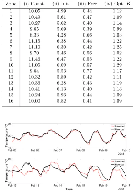
Table 2. RMSE for: (i) constrained optimisa-tion, (ii) constrained optimisation with initial conditions based on physical coefficients, (iii) unconstrained optimisation of [A,B] and (iv)

optimisation of Bonly.

Zone (i) Const. (ii) Init. (iii) Free (iv) Opt.B

1 10.05 4.99 0.44 1.12 2 10.49 5.61 0.47 1.09 3 10.27 5.62 0.40 1.14 4 9.85 5.69 0.39 0.99 5 8.33 4.28 0.66 1.03 6 11.15 6.38 0.44 1.22 7 11.10 6.30 0.42 1.25 8 9.70 5.46 0.56 1.02 9 11.46 6.47 0.55 1.22 10 11.05 6.09 0.57 1.29 11 9.84 5.53 0.77 1.17 12 10.32 5.89 0.42 1.11 13 10.36 6.28 0.43 1.19 14 10.41 6.13 0.40 1.13 15 10.24 5.93 0.44 1.09 16 10.00 5.82 0.41 1.09

Fig. 4. Measured temperatures (solid) compared to the optimised model response (dotted) for an illustrative AHU on A–floor for the first week of February 2018. Upper plot: estimation. Lower: validation experiment.

estimation via a subspace Gauss–Newton or Levenberg– Marquardt least squares search. Figure 4 illustrates a typical model fit when using unconstrained optimisation of [A,B] in this manner, with column (iii) of Table 2 showing the Root Mean Square Errors (RMSE) between the simulated and actual return temperatures. Here, if the purely mechanistic model is utilised the fit is very poor, hence Table 2 only summarises the results for vari-ous optimisation approaches: column (i) uses zero for the coefficient initial values, whilst (ii) utilises the physically– based values of the coefficients developed in section 3.3, demonstrating the value of determining these.

6. CONCLUSIONS

A model of a four-floor building on a university campus has been developed using the thermal–electrical analogy. Physically-derived parameters yield relatively poor perfor-mance, which is improved when the model is combined with occupancy estimation and numerical optimisation of the coefficients using data from the BMS. In this regard, one novelty of the proposed approach is the utilisation of occupancy estimates based on a bespoke combination of wifi and CO2 data. However, to validate the approach

and to compare with other modelling methods from the literature, additional observation days are required and this is the subject of current research by the authors.

An energy centre provides hot water for heating the build-ing, and contains multiple methods of heat production, such as gas boilers and a biomass generator. Therefore, in future research, this type of model will be used to explore options for a hierarchical control system, with a particular focus on optimising the use of the boilers and generator. In this regard, the authors are presently developing demand– side control concepts to address multiple buildings on the network i.e. the control actions for one building are ac-counted for when choosing actions for the other buildings. This will be achieved within a non-minimal state space model predictive control framework (Taylor et al., 2013). Moreover by incorporating weather into the control system and so making full use of the available data from the local Hazelrigg weather station, it is anticipated that the entire network can be better optimised.

REFERENCES

Anderson, A. (2006). Conventions for U–value calcula-tions. BRE Press, BRE Scotland.

Chen, Q., Fu, R.H., and Xu, Y.C. (2015). Electrical circuit analogy for heat transfer analysis and optimization in heat exchanger networks. Applied Energy, 139, 81–92. Foucquier, A., Robert, S., Suard, F., St´ephan, L., and Jay,

A. (2013). State of the art in building modelling and energy performances prediction: A review. Renewable and Sustainable Energy Reviews, 23, 272–288.

Fraisse, G., Viardot, C., Lafabrie, O., and Achard, G. (2002). Development of a simplified and accurate build-ing model based on electrical analogy. Energy and Buildings, 34(10), 1017–1031.

Gorni, D. and Visioli, A. (2017). Genetic-based optimiza-tion of temperature set-point signals for buildings with unoccupied rooms. IFAC-PapersOnLine, 50, 13084– 13089.

Gouda, M., Danaher, S., and Underwood, C. (2002). Building thermal model reduction using nonlinear con-strained optimization. Building and Environment, 37, 1255–1265.

Goyal, S. and Barooah, P. (2012). A method for model-reduction of non-linear thermal dynamics of multi-zone buildings. Energy and Buildings, 47, 332–340.

Goyal, S., Ingley, H.A., and Barooah, P. (2013). Occupancy-based zone-climate control for energy-efficient buildings: Complexity vs. performance.Applied Energy, 106, 209–221.

Kim, S.H. (2013). Building demand-side control using thermal energy storage under uncertainty: An adaptive MMPC approach. Building & Env., 45, 111–128.

Klein, S., Beckman, W., and Cooper, P. (1978).TRNSYS:

A Transient System Simulation Program. Madison,

University of Wisconsin, Solar Energy Laboratory. Kossak, B. and Stadler, M. (2015). Adaptive thermal

zone modeling including the storage mass of the building zone. Energy and Buildings, 109, 407–417.

Luo, M., Wang, Z., Ke, K., Cao, B., Zhai, Y., and Zhou, X. (2018). Human metabolic rate and thermal comfort in buildings. Building and Environment, 131, 44–52. Mayer, B., Killian, M., and Kozek, M. (2017).

Hierar-chical model predictive control for sustainable building automation. Sustainability, 9(2: 264).

Paschkis, V. and Baker, H. (1942). A method for de-termining unsteady-state heat transfer by means of an electrical analogy. Trans. ASME, 64(2), 105–112. Peng, C. and Wu, Z. (2008). Thermoelectricity analogy

method for computing the periodic heat transfer in external building envelopes. Applied En., 85, 735–754. Penman, J. (1990). Second order system identification in

the thermal response of a working school. Building and Environment, 25(2), 105–110.

Price, L., Young, P., Berckmans, D., Janssens, K., and Taylor, C.J. (1999). Data-based mechanistic modelling (DBM) and control of mass and energy transfer in agricultural buildings. Annual Rev. Control, 23, 71–82. Ramirez-Laboreo, E., Sagues, C., and Llorente, S. (2014). Thermal modeling, analysis and control using an elec-trical analogy. In 22nd Mediterranean Conference on Control and Automation. Palermo, Italy.

Tabak, V. and de Vries, B. (2010). Methods for the prediction of intermediate activities by office occupants. Building and Environment, 45(6), 1366–1372.

Tate, O., Wilson, E.D., Cheneler, D., and Taylor, C.J. (2018). Computational fluid dynamics and data–based mechanistic modelling of a forced ventilation chamber. IFAC–PapersOnLine, 51, 263–268.

Taylor, C.J., Leigh, P.A., Chotai, A., Young, P.C., Vranken, E., and Berckmans, D. (2004). Cost effective combined axial fan and throttling valve control of ven-tilation rate. IEE Proceedings D, 151(5), 577–584. Taylor, C.J., Young, P.C., and Chotai, A. (2013). True

Digital Control: Statistical Modelling and Non-Minimal State Space Design. Wiley.

Uribe, O.H., Martin, J.P.S., Garcia-Alegre, M., Santos, M., and Guinea, D. (2015). Smart building: decision making architecture for thermal energy management. Sensors, 15, 27543–27568.

Wolisz, H., Kull, T.M., Streblow, R., and M¨uller, D. (2015). The effect of furniture and floor covering upon dynamic thermal building simulations.Energy Procedia, 78, 2154–2159.

Yang, R. and Wang, L. (2013). Multi-zone building energy management using intelligent control and optimization. Sustainable Cities and Society, 6(1), 16–21.

Yang, Z. and Becerik-Gerber, B. (2014). Modeling per-sonalized occupancy profiles for representing long term patterns by using ambient context. Building and Envi-ronment, 78, 23–35.