Shape Estimation Using Polarization
and Shading from Two Views
Gary A. Atkinson,
Student Member,
IEEE, and Edwin R. Hancock
Abstract—This paper presents a novel method for 3D surface reconstruction that uses polarization and shading information from two views. The method relies on the polarization data acquired using a standard digital camera and a linear polarizer. Fresnel theory is used to process the raw images and to obtain initial estimates of surface normals, assuming that the reflection type is diffuse. Based on this idea, the paper presents two novel contributions to the problem of surface reconstruction. The first is a technique to enhance the surface normal estimates by incorporating shading information into the method. This is done using robust statistics to estimate how the measured pixel brightnesses depend on the surface orientation. This gives an estimate of the object material reflectance function, which is used to refine the estimates of the surface normals. The second contribution is to use the refined estimates to establish correspondence between two views of an object. To do this, surface patches are extracted from each view, which are then aligned by minimising an energy functional based on the surface normal estimates and local topographic properties. The optimum alignment parameters for different patch pairs are then used to establish stereo correspondence. This process results in an unambiguous field of surface normals, which can be integrated to recover the surface depth. Our technique is most suited to smooth nonmetallic surfaces. It complements existing stereo algorithms since it does not require salient surface features to obtain correspondences. An extensive set of experiments, yielding reconstructed objects and reflectance functions, are presented and compared to ground truth.
Index Terms—Polarization imaging, surface shape recovery, stereo, reflectance function estimation, patch alignment.
Ç
1
INTRODUCTION
T
HEproblem of recovering the 3D shape of an object fromone or more views is a central topic in computer vision and is given the generic termshape-from-X. Perhaps the best-known single view technique is shape-from-shading (SFS), where variations in image brightness are used to estimate the field of surface normal directions and, ultimately, the 3D surface geometry. A multi-image extension of SFS is
photometric stereo, where several images are used with a fixed camera position but varying light source directions.
In this paper, we present a novel two-view technique for surface reconstruction based on polarization analysis. The technique uses Fresnel theory to recover the surface normals under conditions of diffuse reflection and establishes the necessary two-view correspondence using surface topogra-phy information. We use polarization measurements ob-tained from a standard digital camera and a linear polarizing filter to accomplish three tasks. First, we estimate the reflectance properties of the material by statistically determining the relationship between the surface orienta-tion (as estimated using polarizaorienta-tion) and the pixel bright-ness. Second, we establish correspondence between the data from the two views using a novel surface-matching algorithm. Finally, the estimated surface normals are used for shape reconstruction.
1.1 Related Work
1.1.1 Shape-from-Shading and Stereo
One of the most extensively studied surface recovery methods is SFS [1]. The foundation of the technique is the relationship between the image pixel brightness and the local surface orientation. SFS aims to estimate the surface normal for each pixel using a single gray-scale image, subject to boundary and smoothness constraints. The height of the surface can then be determined from the resulting field of surface normals (the needle map) using surface integration methods [2], [3].
Despite many attempts to apply it to real-world problems, SFS has found only few successful applications. One reason for this is that, with unknown light sources, an inherent ambiguity known as bas-relief [4] is present, which allows differently shaped objects to produce the same intensity image. Another reason for the lack of success is that the relationship between the incident light source direction and the distribution of reflected light is generally complicated and unknown. This relationship, which is defined quantita-tively later on in Section 3, is termed thereflectance functionor
bidirectional reflectance distribution function (BRDF). The traditional approach adopted in SFS is to assume that
Lambert’s lawapplies. This means that the observed image brightness simply depends on the cosine of the angle between the surface normal and the light source direction. It has long been known, however, that Lambert’s law only works well for matte surfaces and breaks down for rough or shiny surfaces [5].
Treuille et al. [6] overcome the problem of unknown BRDF by placing spherical reference objects in the scene. Surface orientation is then estimated by applying the orientation-consistencyassumption. That is, the surface orientations at
. The authors are with the Department of Computer Science, University of York, York YO10 5DD, UK. E- mail: {atkinson, erh}@cs.york.ac.uk. Manuscript received 13 Mar. 2006; revised 9 Oct. 2006; accepted 2 Jan. 2007; published online 26 Jan. 2007.
Recommended for acceptance by Y. Sato.
For information on obtaining reprints of this article, please send e-mail to: [email protected], and reference IEEECS Log Number TPAMI-0223-0306. Digital Object Identifier no. 10.1109/TPAMI.2007.1099.
points on the unknown object are deduced from those points on the reference object that have identical intensities. Robles-Kelly and Hancock [7] estimate the BRDF from a single image without reference objects by calculating a mapping from a single image onto a Gauss sphere using the cumulative distribution of intensity gradients. A similar orientation-consistency assumption to that used by Treuille et al. is then applied. Ragheb and Hancock [8] use theoretical reflectance models [5] to “correct” the images, so that they appear to be Lambertian. Conventional SFS algorithms are then applied to determine the 3D geometry.
In order to overcome the underconstrained nature of a single-view vision, many researchers have turned to multi-ple-view techniques [9], [10]. If a point in an image from one view is known to correspond to a point in an image from a second view, then triangulation can be used to determine the distance to the camera. The correspondence problem, how-ever, is difficult and is a major hurdle in stereo vision. Jin et al. [11] use shading information from multiple views to for-mulate stereo vision in terms of region correspondence. Many other techniques rely on matching salient image features [12]. In Photometric stereo [13], a fixed camera is used with varying but known light source directions. In certain situations, photometric stereo is possible using three images. The case where the surface is known to be Lambertian is an example of this. However, at least four images are necessary if more complicated reflectance functions are present. Also, more than three images are generally needed to deal with shadows and interreflections and to estimate the albedo. Zickler et al. [14] have used a technique calledHelmholtz stereopsis, where the light source and camera are interchanged. This has the advantage that only two images are needed but requires more precisely controlled experimental conditions.
1.1.2 Polarization Methods
An alternative method for shape analysis relies on the principle that light is partially polarized as a result of surface reflection [15, Section 8.6]. The angle of polarization provides an ambiguous estimate of the surface normal azimuth angle (the angle of the projection of the surface normal onto the image plane), whereas the degree of the polarization constrains the zenith angle (the angle between the surface normal and the viewing direction) [16]. The polarization process is a result of interactions between the incident electromagnetic waves and the directional electron charge density in the medium. An important advantage of polariza-tion visionover SFS is that the azimuth angle is easily recovered up to an ambiguity of 180 degrees. One must know, however, whether the reflection is a direct mirror-like reflection (specular reflection) or a result of subsurface interactions (diffuse reflection). If the reflection type is not known, then there are four possible angles separated by 90 degrees.
A technique that has become a standard in polarization vision is to take digital images of an object using a digital camera mounted with a linear polarizer rotated to different orientations. This was used, for example, by Miyazaki et al. [17] to recover the 3D geometry of transparent objects using specular reflection—a class of material that makes SFS impossible. In an earlier paper [18], the emission of an infrared light was also used. Wolff [19] made the first attempt to combine the polarization data from more than one view, with the aim to estimate the orientation of a
plane. On the other hand, Miyazaki et al. [20] and Drbohlav and Sa´ra [21] apply the theory of polarization to recover shape usingdiffusereflection. Rahmann and Canterakis [22], [23] attempt to account for both reflection types.
In addition to shape reconstruction, polarization has found applications in several other areas of computer vision too. Wolff and Boult [16], Nayar et al. [24], and Umeyama [25] have devised ways to separate diffuse from specular reflection. Wolff and Boult [16] experimented with segment-ing images accordsegment-ing to dielectric/metallic reflectance prop-erties. Drbohlav andSa´ra [26] have enhanced photometric stereo by the addition of constraints from polarization. Clark et al. [27] demonstrate the usefulness of polarization in triangulation-based range scanning, where it is used to distinguish true laser stripes from interreflections. Schechner et al. have demonstrated how polarization can enhance images taken in poor viewing conditions such as haze [28] or underwater [29]. Finally, Shibata et al. [30] use polarization and a range scanner to recover reflectance functions.
The main disadvantage of polarization vision is the experimental difficulty in acquiring the required data. The standard method, mentioned above, requires a minimum of three images from each view, each with a different polarizer angle. This is a time-consuming process and limits the possible applications. It is, however, generally less of a practical hindrance than the steps needed to acquire the images used in a photometric stereo and Helmholtz stereop-sis, since fewer illumination conditions or views are normally required for polarization methods. Wolff [31] and others have improved matters a little by developingpolarization cameras. These devices use liquid crystals to rapidly switch the axis of the polarizing filter. The disadvantage here is that the data has a greater susceptibility to noise. Miyazaki et al. [32] improved the polarization camera by using PLZT (from lead (Pb) lanthanum (La) zirconium (Zr) titanium (Ti)) to switch the polarization state of reflected light.
1.2 Contribution
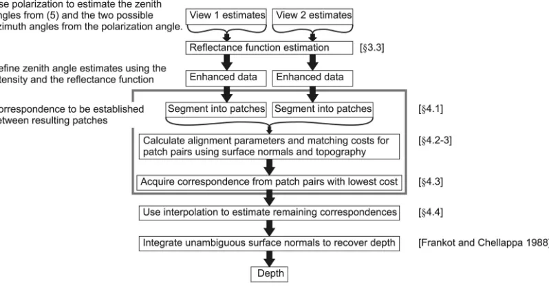
The main aim of this paper is to develop a new method for stereo shape recovery for featureless surfaces. Examples of such surfaces include shiny porcelain, plastics, and painted surfaces. Our motivation is that we cannot rely on traditional stereo techniques that depend on salient surface features for correspondence. We therefore propose a novel method for establishing correspondence that does not rely on feature matching. To accomplish this task, we use polarization to analyze the topographical surface structure and use this information to perform patch matching in order to establish correspondence. To ensure that the results are accurate, we incorporate shading information into the algorithm by means of an estimated reflectance function. This is used to improve the accuracy of the surface normal estimates. Fig. 1 shows an overview of the method diagrammatically and should be referred to throughout the paper.
statistics. This is done because the initial estimates of the surface normals are heavily contaminated by noise and interreflections. For this paper, we concentrate on the case where the light source and the camera directions are identical so that the brightness is independent of the azimuth angle. We also assume that the reflectance is isotropic.
The enhanced, but still ambiguous, surface normals are then fully constrained by establishing correspondence between the two views using patch matching to optimize a cost function. The cost function for this matching process is based on both the normal directions and the local surface topography. The latter property is characterized by the view invariant quantity referred to as theshape index[33]. Surface normals are then integrated to obtain depth using the Frankot-Chellappa method [2]. In principle, triangulation is more accurate, but integration is less sensitive to errors, and our contribution is primarily about surfacenormalestimation. Our method differs from previous shape recovery techni-ques in the following respects: Most importantly, our method is the first polarization-based technique to apply a global reflectance function estimation algorithm to incorporate shading information into the recovery process. Miyazaki et al. [17] use two views and estimate surface orientation from specular reflections. This means that the object had to be placed inside a “cocoon” with several external light sources so that specular reflections occur over the entire object. We also aim to recover denser correspondence here. In [20], Miyazaki et al. are able to use only a single view and therefore have the advantage over our method that less specific measurement conditions are needed. However, they only partially solve the azimuth angle ambiguity, making restric-tive assumptions about the object’s shape histogram. The methods devised by Rahmann and Canterakis [22], [23] use only the azimuth angles to establish correspondence and allow for both specular and diffuse reflection. This potentially results in less noisy reconstructions but at the cost of discarding large amounts of information.
The main weakness of our contribution is that we currently require a somewhat restrictive arrangement of the equip-ment. Most notably, we require that the object is rotated. In
future work, we aim to reduce this restriction by moving the camera (or using two cameras simultaneously) but keeping the light source and object fixed. This would be more difficult since the reflectance function would be a function of both azimuth and zenith angles for at least one of the views.
By contrast to photometric stereo, our method has the following advantages: First, photometric stereo requires three or more images with different light source directions and constant camera positions, whereas our method needs only two views with the light source and camera in the same direction. Second, we do not rely on an assumed reflectance function but, instead, estimate it using global image statistics. Finally, because photometric stereo uses a fixed camera position, there is no obvious way to perform 360 degrees object reconstruction. Our method by contrast, involves a patch-matching procedure, which can be used to combine surfaces from any number of views.
The remainder of the paper is organized as follows: Section 2 introduces the standard Fresnel reflectance theory and explains how this leads to a means to constrain surface normals. Section 3 describes the proposed reflectance function estimation technique and presents results for objects of different shapes and materials. Section 4 presents the multiview polarization-based reconstruction method. Real-world examples of reconstructed shapes are provided in Section 5. Section 6 concludes the paper.
[image:3.612.86.485.79.288.2]2
FRESNEL
THEORY AND
POLARIZATION
VISION
In this section, we present an overview of the standard background theory necessary to understand our novel method. The work is primarily based on the Fresnel theory, which is used to describe how light is polarized when transmitted or reflected from an interface between two media with different refractive indices. We then show how this has been used in computer vision and define some of the quantities used in the remainder of the paper.2.1 Fresnel Coefficients
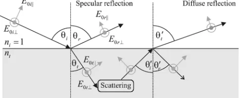
Consider the specular reflection of a ray of light from a surface point, as shown in Fig. 2. Assume that the surface is a smooth interface between a dielectric and air. The Fresnel equations [15, Section 4.6] give the ratios of the reflected wave amplitude to the incident wave amplitude. They can be applied to incident light that is linearly polarized perpendicular to or parallel to the plane of incidence (the plane of the paper in Fig. 2). The ratios depend upon the angle of incidence i and the refractive index nt of the
reflecting medium. We assume that the object is placed in airðni ¼1Þ. Since the incident light can always be resolved
into two perpendicular components, the Fresnel equations are applicable to all incident polarization states. For the work reported here, we use unpolarized incident light.
For the geometry shown in Fig. 2, the Fresnel reflection coefficients are
r?ðni; nt; iÞ
E0r? E0i?
¼nicosintcost
nicosiþntcost
; ð1Þ
rkðni; nt; iÞ
E0rk E0ik
¼ntcosinicost
ntcosiþnicost
: ð2Þ
Equation (1) gives the reflection ratio for light polarized perpendicular to the plane of incidence, and (2) is for light polarized parallel to the plane of incidence. The angletcan be
obtained from the well-known Snell’s law:nisini¼ntsint.
Cameras do not measure the amplitude of a wave but the square of the amplitude orintensity. With this in mind, it can be shown that the intensity coefficients, which relate the reflected power to the incident power, areR?¼r2?andRk¼ r2
k[15, Section 4.6].
Fig. 3 shows the Fresnel intensity coefficients for a typical dielectric as a function of the angle of the incident light. Both reflection and transmission coefficients are shown, where the latter refers to the ratio of transmitted to incident power (the transmission coefficients are simply T?¼
1R?andTk¼1Rk).
2.2 Polarization Analysis
The work reported here relies on taking a succession of images of objects with a polarizer mounted on the camera rotated to different angles. The measured pixel brightness at a given point varies with polarizer angle pol according to
theTransmitted Radiance Sinusoid(TRS)
IðpolÞ ¼
ImaxþImin
2 þ
ImaxImin
2 cosð2pol2Þ; ð3Þ
where Imax and Imin are the maximum and minimum
intensities in the sinusoid, respectively, andis the angle of polarization of the light or thephase angle.
Thedegree of polarizationis defined to be
¼ImaxImin
ImaxþImin
: ð4Þ
It is possible to combine (4) and the Fresnel theory to obtain an expression for the degree of polarization in terms of the refractive index and the zenith angle [16]. The expression, however, is only applicable to specular reflection since the process that causes polarization by diffuse reflection is different, as explained below.
During diffuse reflection [16], a portion of the incident light penetrates the surface and is scattered internally. Some of the light is then refracted back into air and is partially polarized in the process. Fig. 2 illustrates the stages of a diffuse reflection schematically. Snell’s law and the Fresnel
transmissioncoefficients (shown in Fig. 3) can be combined to derive the following equation for the degree of polarization:
ðn; Þ ¼ ðn1=nÞ
2
sin2
2þ2n2 ðnþ1=nÞ2sin2þ4 cospffiffiffiffiffiffiffiffiffiffiffiffiffiffiffiffiffiffiffiffiffiffin2sin2: ð5Þ
[image:4.612.318.509.73.200.2]Here, and for the remainder of the paper, we call the refractive index of the reflecting medium n and use the typical value of n¼1:4. The dependence of the degree of polarizationon the zenith angleis shown in Fig. 4.
[image:4.612.32.275.74.173.2]Fig. 2. Reflection of a ray of light by a medium. Definitions of angles and electric fields are shown.
Fig. 3. Reflection and transmission coefficients for a dielectricðn¼1:5Þ.
[image:4.612.57.248.213.338.2]The azimuth angle of the surface normal is also intimately related to the Fresnel equations. As Fig. 3 shows, the component of the internally scattered light polarized parallel to the plane containing the surface normal and reflected ray is transmitted back into the air most efficiently. The orientation of this plane is therefore the phase angle and is equivalent to the surface azimuth angle. However, since two polarization angles separated by 180 degrees are equivalent, the azimuth angle can only be determined up to an ambiguity. Fig. 5 defines the angles and directions used throughout this paper. We denote the phase angle of the light as, whereas the two candidates for the surface azimuth angleare1¼ and
2¼þ180 degrees. For a fully constrained surface normal,
the Cartesian componentspx,py, andpzare given by
px
py
pz
0 @
1 A¼
cossin
sinsin
cos
0 @
1
A: ð6Þ
The experimental arrangement used for this work is shown in Fig. 6. We concentrate on the case whereL0, that is,
retroreflection. Our experiments are performed in dark room conditions with a single-point light source. For all the work
presented in this paper, gray-scale images of intensitiesI0,I45,
andI90were acquired with the polarizer oriented at 0, 45, and
90 degrees, respectively, where 0 degrees corresponds to vertical alignment. The following equations were then used to calculate the intensity, phase, and degree of polarization, which collectively form thepolarization image[31]:
I¼I0þI90; ð7Þ
¼
1 2arctan
I0þI902I45
I90I0
if I90< I0< I45
00
þ180 if I90< I0 and I45< I0
00
þ90 otherwise;
8 > > < > > :
ð8Þ
¼ I90I0
ðI90þI0Þcos 2
: ð9Þ
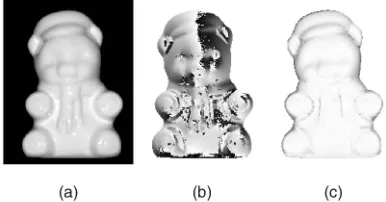
An example of the three components of a polarization image for a white porcelain object (a bear model) is shown in Fig. 7.
[image:5.612.318.511.74.175.2]For all of the results in this paper, we used a Nikon D70 digital single-lens reflex (SLR) camera, with an exposure of 1/30 second and an aperture off5:6. Raw images were stored in gray scale using 256 levels. When the reflectance function estimation technique described below is used, we found that the contribution to the error of the final zenith angle estimate due to camera noise is small compared to the overall uncertainty. (An inexact refractive index estimate and other factors make a greater contribution). This is not always true for the azimuth angle estimates, so we use the average of four
[image:5.612.54.250.75.257.2]Fig. 5. Definition of angles and the two possible surface normals.is used in Section 4.px1andpy1can be calculated using (6) with¼1. Forpx2andpy2,¼2is used.
Fig. 6. Schematic of a polarization image acquisition system. If diffuse reflection is being studied, then the best results are obtained when the lamp is collimated as this reduces reflections from the environment. These effects are minimal when our reflectance function is used.
[image:5.612.124.444.614.731.2]frames before any processing is conducted. We assume that the reflected radiance is proportional to the measured pixel brightness. In fact, experiments show that this is not quite true and there is potential for improving the algorithm by taking the camera response function into consideration.
2.3 Discussion
One advantage of exploiting diffuse reflection compared to specular reflection is that the relationship between the degree of polarization and the zenith angle is one to one for the former reflection type but one to two for the latter [16]. Another advantage is that, assuming the light becomes completely depolarized after surface penetration, then the polarization state of the incident light can be arbitrary for diffuse reflection.
The main difficulties with using diffuse reflection are as follows: First, the data is generally much noisier for diffuse reflection due to the weaker polarizing effects. Second, although the dependence upon the refractive index is not strong for either reflection type, it is weaker for specular reflection. Finally, interreflections between points are mainly specular and cause erroneous orientation estimates if the theory for diffuse reflection is applied.
Both diffuse and specular reflections are affected by roughness. At the microscopic scale, a rough surface can be regarded as a set of facets with Gaussian random orienta-tion. Due to external scattering between these facets and after subsurface scattering followed by re-emission, light impinging on a single element of the camera charge-coupled device (CCD) chip has a distribution of polariza-tion angles. The degree of polarizapolariza-tion is therefore observed to be reduced, resulting in an underestimate of the zenith angle. The azimuth angle estimate remains accurate provided that the mean facet orientation matches the local mean surface orientation.
3
REFLECTANCE
FUNCTION
ESTIMATION
In this section, we present our method for calculating the reflectance function using the zenith angles estimated from the polarization data (5) and the intensity images. The aim is to improve the accuracy of the zenith angle estimates and to reduce the effects of noise, interreflections, and surface roughness. Specifically, we show how the intensity depends on the zenith angle for the case where the camera and light source lie in the same direction. This allows the zenith angles to be estimated from the measured intensities via a lookup table. The method discussed in this section corresponds to the upper part of Fig. 1.
3.1 Preliminaries
The BRDFfði; i; r; rÞof a particular material is the ratio
of the reflected radianceLrðr; rÞto the incident irradiance
Liði; iÞfor the given illumination and viewing directions.
It is measured per unit solid angle per unit foreshortened area and is given by
fði; i; r; rÞ ¼
Lrðr; rÞ
Liði; iÞcosid!
; ð10Þ
whereand, respectively, denote the zenith and azimuth angles, and the subscriptsiandr, respectively, denote the directions of light incidence and reflectance [34, Section 4.2].
For this paper, we work under retroreflection conditions. This means that the light source and camera directions are identical at any given visible point on the surface. In addition, if we assume that the BRDF is isotropic, then the reflected radiance is independent of the azimuth angle . Furthermore, the zenith angles in (10) are equalði¼rÞ.
Therefore, the BRDF depends only onand can be reduced tofðÞ. As a result, the reflected radiance is
LrðÞ ¼fðÞLiðÞcosd!: ð11Þ
If we assume that the target object subtends a small angle with respect to the optical axis of the camera, then the irradiance on the sensing element in the camera (CCD chip) is
LCCD¼
4
AL
A
2
Lr/Lr; ð12Þ
whereALis the lens diameter, andAis the distance between
the lens and the image plane [34, Section 4.2]. As mentioned earlier, we also assume that the camera response function is linear, that is, pixel gray-scale valuesI/Lr(orLCCD).
In effect, we are estimating a unidimensional reflectance distribution function. Since the measured pixel intensity is independent of the azimuth angle under retroreflection conditions, the azimuth angle ambiguity does not compli-cate the reflectance function estimation process. The incident radiance LiðÞ is not generally known since we
work with an uncalibrated light source. We are therefore estimating the reflected radiance up to an unknown constant. However, this constant is unimportant for shape recovery, since we only require the relationship between the surface normal and the measuredpixel brightness.
For our shape recovery algorithm presented in Section 4, we do not use the reflectance functionfðÞdirectly, but the
radiance functionLrðÞ, which incorporates thecosterm (11).
That is, LrðÞ /fðÞcos. For the rest of this section, we
therefore concentrate on the estimation of the radiance function. It is clearly trivial to calculate the reflectance function up to an unknown constant with the radiance function to hand.
Our technique makes use of the 2D histogram of zenith angles and intensities (that is, the observed distribution of the gray-scale values with the zenith angles). The histogram is defined formally as follows: From the polarization data, we have a set of Cartesian pairs (zenith angles and measured pixel brightness), D ¼ fðd; IdÞ;d¼1;2 . . .jDjg, where d is the
zenith angle estimated from (5), andIdis the measured pixel
gray-scale value at the pixel indexedd. We wish to approx-imate the radiance functionLrðÞin terms of a set of discretely
sampled Cartesian pairs, L^r ¼ fðk; IkÞ;k¼1;2 . . .kmaxg,
whereLrðkÞ ¼Ik, and we choosekmax¼100.
The histogram contents for bin ði; jÞ are given by
HCi;j¼ jBCi;jj, whereBCi;j is the subset of D that contains
the Cartesian pairs falling into the relevant bin. This subset is given by
BCi;j¼ ðd; IdÞ;
d 2 ð
binÞ
i w=2; ð
binÞ
i þw=2
h
;
Id 2 Ið
binÞ
j wI=2; Ið
binÞ
j þwI=2
h
8 > < > :
9 > = > ;;
ð13Þ
wherewis the bin size that is arbitrarily chosen to bew¼
90=k
max and wI ¼255=kmax. ðibinÞ and I
ðbinÞ
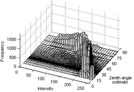
spaced between 0 and 90 degrees and between 0 and 255, respectively. Fig. 8 shows a histogram of the intensities and the zenith angles for the porcelain bear model (for this figure only, unequal bin sizes are used to aid visualization).
3.2 Histogram Interpretation
Before introducing our reflectance function estimation method, we describe a simple experiment that illustrates the structure of the histogram defined above for a real-world example. We also show how the histogram can be interpreted using physical considerations. The footprint of the histogram from Fig. 8 is shown in Fig. 9. Note that there are a small but significant number of pixels that do not fall on or even near the peak frequency curve and that the curve itself is broader than one might initially expect.
Figs. 9b, 9c, and 9d show gray-scale images of the bear model. Pixels falling into the boxes marked in Fig. 9a are highlighted. The first box includes pixels falling onto the peak frequency curve of the histogram. Pixels that fall into boxes 2 and 3 clearly do not follow the general trend and make the task of shape recovery and reflectance function estimation more difficult.
The peak frequency curves found in the histograms are broadened due to roughness, interreflections, and noise. As
explained in Section 2.3, roughness tends to depolarize light, reducing the estimate of the zenith angle. The bear model used in Fig. 9a is relatively smooth, but later, we show examples of rougher surfaces, where the curve is broadened further. The more distant outliers in the histograms are caused by interreflections. These occur where light from a source is specularly reflected between two points on the surface and then toward the camera. This interreflection process obeys the theory for specular reflection, although a small diffuse component will generally be present also.
The exact effect of an interreflection depends upon its strength. If it is weak, then the diffuse component still dominates. The degree of polarization and, hence, the zenith angle estimate will be reduced since the phase angle of specularly reflected light is perpendicular to that of diffuse reflections. This process can be seen in box 2 of Fig. 9. Here, a small specular component is present due to reflections from the table on which the object rests. For strong interreflections, the specular component dominates. Since the polarizing properties of specular reflection are greater than that for diffuse reflection, we have a situation where the degree of polarization exceeds that which would be expected for any purely diffuse reflection (box 3). Careful examination of the ears of the bear model in Fig. 9c shows a regionsurroundingan interreflection where the specular component is weaker.
Notice that, apart from the few cases where the strong interreflection limit is met (as in box 3), the degree of polarization is always equal to or less than the value expected for a given zenith angle. This is substantiated by the fact that the exact curve (measured using an object of the same material but known to have cylindrical shape) approximately follows the outer envelope of the histogram. This was verified with other objects.
3.3 The Proposed Method
[image:7.612.37.271.74.236.2]Based on the premise above, the radiance function is estimated by fitting a curve to the outer envelope of the intensity-zenith angle histogram. The proposed method allows for some strong (box 3 type in Fig. 9) specular interreflections, but we do assume that these do not cover a large fraction of the surface. Only one view is strictly necessary for this section, although the method described in
Fig. 8. Histogram showing the frequency of occurrence of intensity-zenith angle pairs for the polarization image of the bear model in Fig. 7.
[image:7.612.79.493.577.732.2]Section 4 requires two views (with identical lighting). For this reason, we include pixels from both views in the setD. Experiments to estimate the radiance function from a single view were found to give similar results.
An initial estimate of the radiance functionL^r¼ fððk1Þ; I
ð1Þ
k Þg
can be obtained using the mean intensity for regularly spaced zenith angle columns of the histogram, that is
kð1Þ¼kðbinÞ; Ikð1Þ¼ Pkmax
j¼1HCk;jIð
binÞ
j
Pkmax
j¼1HCk;j
: ð14Þ
The same number of bins ðkmaxÞ are used for sampling
zenith angles and intensities. It turns out that our algorithm is not critically dependent on this initial estimate and, so, we aim for maximum computational efficiency at this point. Next, we need the outer envelope of the histogram. The algorithm obtains this by extracting a one-dimensional (1D) histogram slice from HCi;j along the straight line that is
perpendicular to the initial estimate at each point k. Histogram values along this line are taken from a linear interpolation of HCi;j. Fig. 10a shows such a histogram for
the straight line shown in Fig. 11a. This histogram data is then fitted to a Weibull probability density function [35, Chapter 1], which is given by
gðqj; ; Þ ¼ q
1
expq q
0 q < ;
(
ð15Þ
whereis a scale parameter, is a shape parameter, and
is a location parameter (not the mean). The corresponding cumulative distribution function is
Gðqj; ; Þ ¼ 1exp
q
q
0 q < :
(
ð16Þ
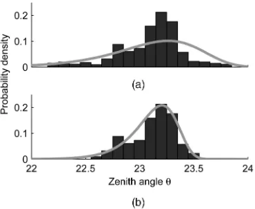
The Weibull distribution is primarily used in lifetime and failure analysis. It is used here since we expect most pixels to fall near the main curve in the 2D intensity-zenith angle histogram. However, due to roughness and interreflections, we also expect more pixels to be located on the left-hand side of the crest (in Fig. 8) than the right-hand side. The 1D histogram slice shown in Fig. 10 justifies this since there is a sharper cutoff on the right-hand side of the histogram.
The fitting process yields parametersðopt1Þ,
ð1Þ
opt, and
ð1Þ
opt.
One option to obtain the Cartesian points in our radiance functionL^r¼ fðð
finÞ
k ; I
ðfinÞ
k Þgis to use
ðkfinÞ¼argmax
g jðopt1Þ;
ð1Þ
opt;
ð1Þ
opt
; ð17Þ
IðkfinÞ¼Ik
kþ1k1
Ikþ1Ik1
ðkfinÞk
; ð18Þ
where (18) is on the straight line perpendicular to the initial radiance function estimate. However, as Fig. 10a shows, the data is not always unimodal and contains outliers, especially in the presence of interreflections. We therefore add the following robust fitting step. If is the lower limit of a bin on the 1D histogram andwis the bin size, then the data is discarded for bins that satisfy
Z þw
g jðopt1Þ; optð1Þ; optð1Þd <0:1; ð19Þ
where w is chosen such that the number of bins is fixed at kmax.
The probability density function parameters are then re-estimated iteratively until convergence to giveðoptitÞ, ðoptitÞ, and
[image:8.612.61.246.71.223.2]ðoptitÞ. Condition (19) is applied after each iteration. We found,
Fig. 10. Histogram of data along the fitting direction shown in Fig. 11a. (a) Initially, the fit is poor. (b) When the low-probability data is discarded using (19), the remaining data closely follows a Weibull distribution.
[image:8.612.106.463.580.725.2]empirically, that the parameters converge after only few (4) iterations.
The outer envelope can then be taken as
ðkfinÞ¼:G jðoptitÞ;
ðitÞ
opt;
ðitÞ
opt
¼0:99; ð20Þ
where (18) is used to obtain the associated IkðfinÞ. In other words, the point where the cumulative probability density function reaches 99 percent is regarded as the outer envelope. The choice of 99 percent is somewhat arbitrary, and it is possible that the algorithm would give better results if the value was fine tuned depending on the material (for example, if the material is known, then an experiment with a sphere or cylinder may help to obtain an optimum value). This is particularly true for rougher surfaces. In the case of smooth surfaces with no noise, the fitted PDF is very narrow so the exact choice of threshold has little impact on results.
Finally, the discretely sampled radiance function L^r is
smoothed using moving averages. Since the relationships between the intensity and zenith angles are usually simple for retroreflection (monotonic, continuous function, continuous derivative, and so forth), we can apply the smoothing at a moderately intense level. Fig. 11b shows the result of the smoothing process. The figure also shows the effect of different refractive indices on the estimated reflectance function between two extreme values. Note that the curves are similar for high refractive indices but deviate further for lower values. Finally, we apply the constraint that lim!90LrðÞ ¼0to estimate the reflectance function at very
large zenith angles [5].
3.4 Measured Reflectance Functions
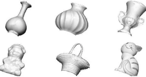
[image:9.612.100.466.76.220.2]A set of porcelain objects, together with estimates of their radiance functions, are shown in Fig. 12. The objects are made from similar types of porcelain and all have smooth surfaces. The cat model is also partially painted and is used to investigate how areas of different albedo affect algorithm performance. The first point to note is that all the objects gave similar radiance functions, which closely matched the exact curve.
Fig. 13 shows that pixels of the painted areas of the porcelain cat model fall well within the envelope of the histogram. This meant that the algorithm recovered the radiance function of the porcelain, whereas the smaller painted areas were disregarded by the robust fitting method.
Note, however, that the algorithm does not always recover the radiance function of the most prevalent color/material. For example, suppose that most of the cat model was red but that some areas were white. The results would then be strongly affected by both red and white areas. Further investigation of textured objects is out of the scope of this paper. In future work, we hope to segment images according to spectral composition, allowing several reflectance func-tions to be estimated.
Fig. 12 also compares the results obtained to the physics-based model developed by Wolff [36], which accounts for multiple subsurface scattering using a Fresnel attenuation factor (based on the same theory as that presented in Section 2). This model uses a scattering theory originally derived for radiative transfer to model the distribution of scattered light within a medium. According to Wolff, the BRDF is
fði; r; nÞ ¼%ð1Fði; nÞÞ 1F arcsin
sinr
n
;1 n
;
ð21Þ
where % is called the total diffuse albedo, and F is the Fresnel function given by
Fði; nÞ ¼
1 2
sin2ðitÞ
sin2ðiþtÞ
1þcos 2ð
iþtÞ
cos2ð
itÞ
; ð22Þ
wheren¼ ðsiniÞ=ðsintÞ (Snell’s law).
Fig. 12. Estimates of the radiance function of the selection of porcelain objects shown to the right (and the bear model from Fig. 9) compared to the exact curve (thick line) and the Wolff model (broken line). The recovered curves were linearly extrapolated to¼0.
[image:9.612.295.536.594.713.2]Since we are studying the case where i¼r, the two
Fresnel terms in (21) are equal. Allowing for the foreshorten-ing effects of orthographic imagforeshorten-ing, (21) then simplifies to
I¼cosð1Fð; nÞÞ2; ð23Þ
whereis a normalizing constant. We use this equation in Fig. 12, whereis selected to give the best agreement with the exact curve, which is also shown in the figure. Note that the use of reflectance models requires estimates of various surface or material parameters, whereas our method needs only an approximate value of the refractive index.
We have also applied our method to various slightly rough surfaces. Examples of which are shown in Fig. 14. Results are generally reasonable, although the estimated radiance curves tend to be least reliable for small zenith angles, where the radiance function is often overestimated.
4
RECONSTRUCTION FROM
TWO
VIEWS
In this section, we describe our method for shape estimation from two views. The goal is to establish and use dense stereo correspondence to resolve azimuth angle ambiguities pre-sent in the surface normal estimates from a single view. The first step is to extract surface patches from the polarization images. These patches are then aligned using an optimization scheme to obtain correspondence indicators. The error criterion is similar to those developed by Cross and Hancock [37] using the EM algorithm and Chui and Rangarajan [38] using softassign.
The input to this stage of the algorithm is the set of ambiguous surface normal azimuth angles from the phase images together with their zenith angles from the estimated radiance function and the raw intensity images. We use the setup shown in Fig. 6 with polarization images taken from two views. For the second view, the turntable is rotated byrot
about thex-axis (see Fig. 6 for the coordinate axis convention). In this paper, we use a known value ofrot¼20.
The set of surface patches are obtained by segmenting the two polarization images into regions1according to the estimated surface normals. The segmentation is performed
using a bithreshold technique, where normals falling into an angular interval are selected from each image. The angular interval is shifted byrotbetween images to account
for the object rotation. Details of this procedure can be found in Section 4.1.
The correspondence problem is then reduced to matching patches from the two views. The solution is to align patch pairs for which a potential correspondence exists. We adopt a dual-step matching procedure in which both correspondence indicators and alignment parameters are sought. The cost function uses the correspondence indicators to gate contribu-tions to a sum-of-squares alignment error for corresponding points. The alignment error measures the difference in the surface normal components and a scale invariant measure of surface topography (the shape index). The matching cost is calculated for all potentially corresponding patch pairs, and the combination that gives the lowest total cost is taken as the set of patch correspondences. The derivation of the cost function that we adopt is given in Section 4.2. The matching algorithm itself and how it leads to unambiguous azimuth angles is described in detail in Section 4.3.
After this process, some areas of the images remain without detected correspondence. Monotonic interpolation is then used to estimate correspondences for such areas. This stage of the method is detailed in Section 4.4. Finally, the Frankot-Chellappa surface integration method is ap-plied to recover a depth map from the field of unambiguous surface normals. In the remainder of this section, we furnish details of the steps described above. Refer back to Fig. 1 for a schematic of the overall algorithm structure.
4.1 Segmentation
The purpose of this stage of the algorithm is to segment the two images into regions that are suitable for establishing correspondence. The segmentation is performed according to the angle defined by
¼arctanðsintanÞ: ð24Þ
[image:10.612.91.476.74.244.2]This is the angle between the viewing direction and the projection of the surface normal onto the horizontal plane (the y-z plane in Fig. 5). If the correct azimuth angle is greater than 180 degrees, then is negative, that is, the surface normal vector points to the left from the viewer’s perspective. However, we do not know the sign ofat this
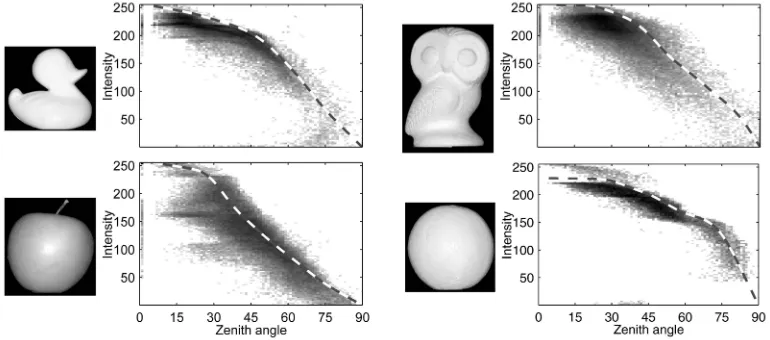
Fig. 14. Histograms and radiance functions for a slightly rough plastic duck, a plaster owl, an apple, and an orange.
point so we can only calculate the modulus of the angle from the estimated phase, that is,jj ¼arctanðsintanÞ.
The zenith angleis determined by the radiance function (11), estimated using the technique from Section 3.3. Let the minimum angle for reliablejjestimates belim. Empirically,
we found thatlimwas approximately 20 degrees for perfectly
smooth objects. For rougher surfaces, a reasonable recon-struction was possible using this value, but results were better when lim¼30 was used. We know that for the regions
where <0for both images, then, where the pixels in the right-hand image (view 2 in Fig. 6) satisfy the condition
limþrot<jj 90; ð25Þ
the corresponding pixels in the left-hand image (view 1) must satisfy the condition
lim<jj 90rot: ð26Þ
Conversely, where >0, then for the regions of the right-hand image that satisfy the condition in (26), the pixels in the corresponding left-hand image regions must satisfy the condition in (25).
Our region segmentation algorithm makes two image passes for each view. On the first pass, the right-hand image is
thresholded using the angle condition in (25), whereas the left-hand image is thresholded using the condition in (26). On the second pass, the angle conditions are interchanged between the left and right-hand views. This two-pass thresh-olding gives two sets of regions per view. Fig. 15 illustrates the possible correspondence combinations between region sets. In this way, we impose angle interval constraints on the allowable region correspondences. Fig. 16 shows a real-world example of the result of the segmentation process.
4.2 Cost Functions
As already mentioned, the algorithm seeks patch corre-spondences so as to minimize a cost (or energy) function. In this section, we first describe a rudimentary cost function based purely on local patch reconstructions. We then introduce a more complex cost function based directly on the estimated surface normals and the scale invariant topographic quantity known as the shape index.
4.2.1 A Rudimentary Cost Function
This cost function is based on the similarity between local patch reconstructions obtained by applying the Frankot-Chellappa method to recover surface depthhfrom needle maps [2]. Fig. 17 shows patch reconstructions from two of the larger regions from Figs. 16a and 16b, using <0.
Consider the alignment of two patches defined by sets of pointsU ¼ fua;a¼1;2 . . .jUjgandV ¼ fvb;b¼1;2 . . .jVjg,
where ua¼ ðxðauÞ; yaðuÞ; zðauÞÞ T
and vb¼ ðxðbvÞ; y
ðvÞ
b ; z
ðvÞ
b Þ T
. The alignment is performed by applying a transformation function J to patch U to obtain the set of transformed positionsU ¼ f^ u^ag, whereu^a¼ ðx^ðauÞ;y^ð
uÞ
a ;z^ð
uÞ
a Þ T
.
[image:11.612.107.459.68.311.2]For our case, where the target object has undergone a known rotation about the vertical axis (x-axis), the transformation contains a y-translation of y, a z -transla-tion ofz, and a rotation about thex-axis of rot. For our
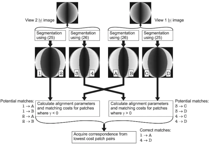
Fig. 15. Flow diagram of the segmentation and correspondence part of the algorithm, using a synthetic sphere as an example. This figure corresponds to the large box in Fig. 1.
[image:11.612.31.272.640.729.2]particular transformation, therefore, x^ðuÞ
a ¼xðauÞ8a2
f1;2 . . .jUjg. We represent the transformation parameters as ¼ ðy;z; rotÞT, where rot is known. Our task then
becomes that of estimating the vector of parameter values
for each potentially corresponding patch pair that mini-mizes an energy functional.
The rudimentary energy functional for aligning patches U andVis
"UVðÞ ¼ PjUj
a¼1
PjVj
b¼1mabðÞjvbu^aðÞj2
PjUj
a¼1
PjVj
b¼1mabðÞ
; ð27Þ
where mabðÞ are the elements of the correspondence
indicator matrixMðÞ, defined below. This is a modified version of the least squares alignment parameter estimation problem. The correspondence indicators exclude the con-tributions to squared alignment error from nonmatching points. Similar cost functions are obtained by Cross and Hancock [37] and Gold et al. [39]. In this paper, the elements of the correspondence indicator matrix are assigned as follows:
mabðÞ ¼ 1 if
a¼argmin
a02AðbÞ
^
yðau0ÞðÞ y ðvÞ
b or
b¼argmin
b02BðaÞ
^
yðuÞ
a ðÞ y
ðvÞ
b0 8 > > < > > : 0 otherwise;
8 > > > > < > > > > :
ð28Þ
whereAðbÞ ¼ fa21;2 . . .jUj jxðuÞ
a ¼x
ðvÞ
b gis the set of labels
for points inUthat lie in the same horizontal plane as point
vb. Similarly, BðaÞ ¼ fb21;2 . . .jVj jxðbvÞ¼xðauÞg are the
labels for points in V in the same plane as point ua. In
other words, mabðÞ ¼1 if vb is the closest point in V to
^
uaðÞ in they-direction within the same horizontal
cross-section. Similarly, mabðÞ ¼1 also if u^aðÞ is the closest
point inUð^Þtovb. The construction of the matrixMðÞis
illustrated in Fig. 18. Note that it does not include a term with the difference in thez-position. This is because, in the final algorithm, the energy functional is given in terms of the surface normals, so the height reconstruction (difference inz-position) is not needed to establish correspondence.
The matrixMðÞis hence defined in a similar fashion to the correspondence matrix used by Chui and Rangarajan [38]. Note that Chui and Rangarajan assume that the correspon-dence is one to one, meaning that each row and each column of the final correspondence matrix has exactly one element set to unity. We do not enforce this constraint here.
Using the correspondence indicator matrix defined in (28) means that any points in nonoverlapping areas of the patches are inappropriately included in the energy calculation. We
therefore use a reduced correspondence matrixM0ðÞwith elementsm0
ab, which is defined by
m0abðÞ ¼
mabðÞ if
min
a02AðbÞ ^y ðuÞ
a0 ðÞ
n o
< yðbvÞ < max
a02AðbÞ y^ ðuÞ
a0 ðÞ
n o
and
min
b02BðaÞ y ðvÞ
b0
n o
<y^ðuÞ
a ðÞ< max b02BðaÞ y
ðvÞ
b0 n o 8 > > > < > > > :
0 otherwise:
8 > > > > > > < > > > > > > :
ð29Þ
This reduced correspondence indicator matrix therefore discards points in the patches where there is no overlap, as shown in Fig. 18.
Note that this method is an alternative to the iterated closest point (ICP) algorithm [40]. We do not use ICP because that method would restrict our cost function to be based on the location of points in 3D space. Although the use of (27) specifically has no advantage over ICP in this respect, we would ideally like to base our cost primarily on the surface normals, rather than on patch reconstructions, to avoid error propagation.
4.2.2 An Improved Cost Function
We aim here to refine the cost function to include surface normal information. However, if only the surface normals are used, then we encounter a problem: It is possible that two surface points on different patches could have identical surface normal directions but very different local shapes. We therefore introduce the shape index into the energy functional to account for local surface topography.
The shape index s is a view-invariant quantity that describes the local topography of a surface and falls in the interval½1;þ1. Wheres¼ 1, the local surface shape is a concave spherical cup, wheres¼0, a saddle point is found, and wheres¼ þ1, the surface takes the form of a spherical dome. Between these values, the surface takes intermediate topographic forms. The shape index is undefined for planar surfaces.
The starting point for the derivation of the shape index is the Hessian matrix, defined by
H¼ @2h=@x2 @2h=@x@y
@2h=@x@y @2h=@y2
¼ @p
0
x=@x @p0x=@y
@p0
y=@x @p0y=@y
[image:12.612.299.534.74.162.2]
; ð30Þ
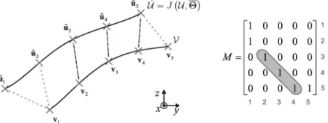
Fig. 18. Illustration of how matricesMðÞandM0ðÞare constructed. The points shown are from a horizontal cross-section of two patches. All broken lines correspond to elements ofMðÞset to unity. ForM0ðÞ only the dark broken lines correspond such elements. The elements of
MðÞare shown to the right. For the reduced correspondence matrix, all elements are zero except for those highlighted.
[image:12.612.52.257.79.162.2]where hðx; yÞ is the surface height. p0x and p0y are the gradients of the surface and are related to the Cartesian components of the unit surface normal in (6) byp0x¼ px=pz
andp0
y¼ py=pz.
The Hessian matrix can be calculated from the normals estimated using polarization data and the radiance func-tion. Since we are performing a differentiation, the estimate of H is not entirely robust to noise. However, since the Hessian will not form the main part of our cost function (the normals themselves do), this problem is not severe.
Using (30) directly leads to a view-biased estimate of the Hessian, due to a foreshortening effect. We therefore introduce the viewpoint-compensated Hessian derived by Woodham [41]
C¼ ffiffiffiffiffiffiffiffiffiffiffiffiffiffiffiffiffiffiffiffiffiffiffiffiffiffiffiffiffiffiffiffiffi1 ð1þpx2þpy2Þ3
q p
2
yþ1 pxpy
pxpy p2xþ1
H: ð31Þ
The eigenvalues of this matrix are
max¼
1
2ðc11þc22SÞ; ð32Þ
min¼
1
2ðc11þc22þSÞ; ð33Þ
where S¼ ffiffiffiffiffiffiffiffiffiffiffiffiffiffiffiffiffiffiffiffiffiffiffiffiffiffiffiffiffiffiffiffiffiffiffiffiffiffiffiffiffiffiffiffiffiffiffiðc11c22Þ2þ4ðc21c12Þ
q
, and cij denotes
ele-ments of C. max and min are the principle curvature
directions at the surface point and are the sole variables in the definition of shape index
s¼2
arctan
maxþmin
maxmin
: ð34Þ
In our energy functional, we motivate the use of the difference in shape index between surface points as follows: Consider two surface points with identical normal direc-tions with one lying on a spherical domeðs¼ þ1Þand the other on a spherical cup ðs¼ 1Þ. The difference in shape index is thenþ2, which increases the matching cost. Based on this observation, we propose the following form, which incorporates both the shape indices and the surface normals
"UVðÞ ¼
PjUj
a¼1
PjVj
b¼1m0abðÞPabðÞs2ab
PjUj
a¼1
PjVj
b¼1m0abðÞ
; ð35Þ
wherePabðÞ ¼ ðpxbp^xaðÞÞ
2
þ ðpybp^yaðÞÞ
2
þ ðpzbp^za
ðÞÞ2andsab¼sbsa.
The “hat” notation is used to represent quantities having undergone transformationJ as before. Note that the shape index does not depend on the transformation parameters since it is rotation invariant. MatrixM0ðÞis calculated in the same way as before, using the Frankot-Chellappa method to determine the nearest neighbors in they-direction. Note that the reconstruction is effectively used only as a means to account for foreshortening (that is, so that patch U can be rotated byrot).
4.3 Final Algorithm
The optimum alignment parameters for patchesUandVare given by
UV ¼argmin
"UVðÞ: ð36Þ
For each pair of corresponding patches W and W0, the correspondence matrix is MðWW0Þ. The matching cost
"UVðUVÞ is calculated for all potential matches. The
algorithm sorts the list of costs into an ascending order (that is, the most confident match first) and confirms the matches sequentially but rejects those that do not satisfy the following consistency constraint:
If a point at they-positionyðuÞ
a corresponds to a point aty
ðvÞ
b , then two other corresponding points at yðuÞa0 andyðvÞb0 must
satisfy
sgn yðuÞa0 yðuÞa
¼sgn yðvÞb0 y
ðvÞ
b
: ð37Þ
Due to occlusion, not all patches have a correspondence at all, so we ideally require a cost threshold. Any matches with a cost above the threshold are then discarded. At present, we are yet to develop an adaptive means of setting this threshold.
The algorithm was first tested using (35) as the energy functional. One problem encountered when using (35) is that an area of a patch may be occluded in one view but not in the other. Another issue is that, even though (35) only needs the Frankot-Chellappa method as a convenient way to account for foreshortening, it still introduces a distortion in the patch shape and, therefore, a nonoptimal correspon-dence matrix. We reduce the impact of these problems by replacing (35) with the following functional, which takes the median energy of the separate costs for each horizontal cross-section of the patches:
"UVðÞ ¼
1
KðÞmedianx2‘
PjUj
a¼1
PjVj
b¼1m00abð; xÞPabðÞs2ab
PjUj
a¼1
PjVj
b¼1m00abð; xÞ
!
:
ð38Þ
Here, ‘¼ fxugTfxvg is the set of unique x-positions
covered by both patches and
m00abð; xÞ ¼ m
0
abðÞ if xðauÞ¼x
ðvÞ
b ¼x
0 otherwise:
ð39Þ
We have also introduced the quantityKðÞ, which rewards patch overlap
KðÞ ¼ PjUj
a¼1
PjVj
b¼1m0abðÞ
PjUj
a¼1
PjVj
b¼1mabðÞ
: ð40Þ
It is not necessary for the algorithm to calculate the cost for every conceivable pair of patches. This is because we know that the two pixels in any given correspondence pair lie on the same horizontal scan line for our particular experimental arrangement. Instead, it only calculates the cost of patch pairs where there is some overlap in the vertical coordinates (that is,‘6¼ ). For such pairs,"UVðÞis
minimized using the Nelder-Mead method [42].
After the patch matching is complete, we can disambig-uate the azimuth angles for the regions where correspon-dence was established. We do this using the knowledge that the patches reconstructed using >0have <180(that is,
¼1 in Fig. 5) and patches where <0 have >180 ð¼2Þ. Fig. 19a shows these unambiguous regions for the
bear model images. We still have two estimates of these unambiguous surface normals, one from each view. Our final value is taken from the view where the zenith angle was greatest since the raw polarization data would have con-tained less noise for this estimate.
4.4 Correspondence for Remaining Areas
Large areas of the images remain without correspondence after the above matching procedure and, thus, remain ambiguous. To assign a value for the azimuth angle for these areas, we usepiecewise cubic Hermite interpolating polynomials
(PCHIP) [43]. This form of interpolation is similar to the spline technique in that a continuous curve is generated that passes exactly through the data points. The difference is that the spline maintains continuous first and second derivatives, whereas PCHIP allows discontinuities in the latter. The advantage of this, from our point of view, is that PCHIP ensures that a monotonic curve is generated, thus, ensuring point correspondences satisfy the condition in (37).
The algorithm effectively plots the y-positions of corre-sponding points from each view against each other and applies PCHIP to interpolate between correspondences. This method only provides relatively crude correspondence for areas not in the vicinity of the regions disambiguated previously. This is one reason for us currently relying on integration methods to recover depth instead of triangula-tion. However, it is sufficient as a means of selecting the most reliable azimuth angle (1or2) for most image pixels.
To demonstrate the effects of disambiguation errors and to further motivate our choice of the Frankot-Chellappa algorithm for shape reconstruction from surface normals,
consider Fig. 20. For this figure, a synthetic sphere was created, and the surface normals were calculated at each point. For a slice of the sphere, the signs of thepx and py
values were changed to simulate the effects of a correspon-dence error. The surface normals were then integrated using the Frankot-Chellappa method to obtain a depth map. The difference between the original sphere and the recovered depth is shown in the figure and is clearly relatively small, given the magnitude of the error introduced. Had triangula-tion been used with such an error, then the reconstructriangula-tion would be more severely deformed.
We do not use the results of PCHIP for areas of the image where jj< rot. Instead, we propagate from surrounding
areas and align surface normals to the mean of local 33windows. This is advantageous since these areas are the most susceptible to noise due to lower degrees of polarization. Fig. 19b shows the unambiguous azimuth angles for the full image for each view.
[image:14.612.111.456.76.171.2]5
RESULTS
Fig. 21 shows the recovered depth maps of some of the objects used in Section 3. They were obtained by applying the Frankot-Chellappa algorithm to the recovered needle maps. A reasonable estimate is made in each of the six cases. There are two poorly recovered object areas. First, the paws of the bear model do not protrude as they should due to interre-flections. Although using the estimated radiance function helped to accurately recover the zenith angles here, the azimuth angles were incorrect for these areas. Second, the handle of the basket does not arch from one side of the object to the other as a result of the needle map integration method. Results for three other objects of different materials are shown
[image:14.612.298.533.601.725.2]Fig. 19. (a) Azimuth angles of disambiguated regions of the bear model. (b) Final estimates of azimuth angles for entire image.
Fig. 20. Illustration of the effects of an incorrect disambiguation in recovered height. (a) Image of py for a synthetic sphere with a disambiguation error introduced. (b) Magnitude of the error in recovered height expressed as a percentage of the radius.
[image:14.612.65.242.638.720.2]in Fig. 22. Here, the original red, green, blue (RGB) images have been used to reapply the texture onto the reconstruction. This final step is for aesthetic purposes only since we do not have full illumination control.
Fig. 23a shows ground-truth cross-sections of the porcelain vase compared to the recovered height. The ground truth was calculated using the volume of revolution of the object contour. The comparison proves that the method works well for the simplest case, namely, that of a smooth object with basic geometry. The difference image between the ground truth and the recovered height is shown in Fig. 23b. Note that any symmetries in the true object geometry are not always preserved in the error. This is a result of small environmental interreflections and is possibly accentuated by imperfect polarizer calibration. For comparison, Fig. 23c shows the difference image when the raw zenith angle estimates were used (that is, those calculated directly from (5) without estimating the radiance function). The root-mean-square height errors were 8 units when the radiance function was used and 18 units when it was not used. Note that the depth of the vase is 150 units. Fig. 24 shows a comparison of the ground truth profiles of the porcelain urn and the orange. The urn profile shows that, although the general shape is recovered, the height variations are less pronounced than they should be for objects with complicated geometry. The method performed better for the orange. Fig. 24b also shows the profile estimate of the orange without using the radiance function. Here, the radiance function was clearly essential for accurate shape estimation.
The method has been tested on a greater range and number of objects than in most of the previous contributions, and the results show several strengths and weaknesses. When the
algorithm is applied to objects with complicated geometry, our method is less accurate than those that use specular reflection such as that in [17]. This is mainly due to higher degrees of polarization associated with specular reflection. As mentioned previously, however, specular reflection is often difficult to measure for an entire surface or scene. Our method has a more general and complete disambiguation than that in [20] and allows reconstructions from different views but gives less accurate results in some cases. Compared to SFS, our method has stronger constraints, and the results are generally superior, although less general to illumination conditions. For cases where triangulation is possible, those methods are more accurate, provided that correspondences are reliable. For this reason, we will consider a combined integration and triangulation final step for future work.
6
CONCLUSION
[image:15.612.35.273.74.132.2]We have devised a new shape recovery technique that combines polarization, shading, and stereo information. Polarization images are acquired from two views of an object on a turntable. The first part of our proposed algorithm estimates the reflectance function of the object under study. This is accomplished globally using the distributions of the initial zenith angle estimates and the pixel brightnesses. Using ambiguous surface normal estimates from the polar-ization images and refined using the estimated reflectance function, the proposed algorithm then establishes stereo correspondence between the views. This task is accomplished using an optimization scheme, where the cost function is based on the surface normals and the shape index. Our results show that the technique is applicable to smooth objects composed of a variety of materials with a known value of the refractive index. The fact that the refractive index must be
Fig. 22. Recovered shape of objects of different materials with the original textures mapped onto the surface.
[image:15.612.295.537.74.125.2] [image:15.612.111.459.596.725.2]