Reducing labeled data usage in duplicate detection using deep belief networks

(1)

MASTER THESIS

Reducing labeled data usage

in duplicate detection using

deep belief networks

Stefan C._Janssen

[email protected]

Faculty of Electrical Engineering, Mathematics and Computer Science Human Media Interaction Research Group

Committee: dr. MannesPoel

dr.ing. GwennEnglebienne drs. Manuelvan den Berg

(2)

(3)

Abstract

Modern duplicate detection systems typically use supervised machine learning algorithms to create duplicate detection models. These algorithms require a large amount of manually labeled data to train on. Using semi-supervised deep learning techniques would allow the training to use not only labeled data, but also unlabeled data, which is easily available. The expectation is that this will allow models with less manually labeled data to achieve similar or better accuracy as traditional supervised algorithms.

To determine the effect of semi-supervised learning, we created several variations of existing duplicate detection algorithms, all focused on incorporating semi-supervised learning. For the matching phase this resulted in a deep belief network instead of a traditional neural network as classifier. Additional variants were also created with word embedding and word hashing as extra features, as both are new developments in natural language processing and often used in combination with deep learning. For the indexing phase semantic hashing was used as a way to encode these additional features.

All these algorithms have been evaluated against several traditional duplicate detection algorithms on two different datasets. Both datasets are samples of real-life datasets and contain contact data. A separate dataset was used for tuning. The different algorithms, covering both the indexing and matching steps in duplicate detection, are compared using a 5x2 K-fold evaluation to determine their performance on unseen data.

The results for the matching step show significant differences between supervised and semi-supervised in only one scenario (improving the F1-score from 0.806 to 0.821). There are no significant differences for the variants which combine semi-supervised learning with the additional features. For the indexing algorithms semi-supervised training does improve the results significantly in several cases (e.g. improving the F1-score from 0.702 to 0.710 in one of cases).

The required modifications in structure have been evaluated separately. The additional auto-encoder layer in matching improves the quality on one of the datasets (e.g. improving the F1-score from 0.919 to 0.935 in one of the cases). For the indexing algorithms the additional semantic hashing reduces the quality (e.g. from F1-score of 0.720 to 0.702 in one case).

(4)

(5)

List of Tables

4.1 Overview of the deep learning based matching algorithm variants. . . 22

4.2 Overview of the hyperparameter configuration for each of the matching variants . 23 4.3 Overview of the deep learning based indexing algorithm variants. . . 26

4.4 Overview of the hyperparameter configuration for each of the indexing variants. . 27

4.5 Overview of the datasets used. . . 28

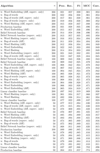
5.1 K-fold evaluation results of the matching algorithms on dataset R. . . 30

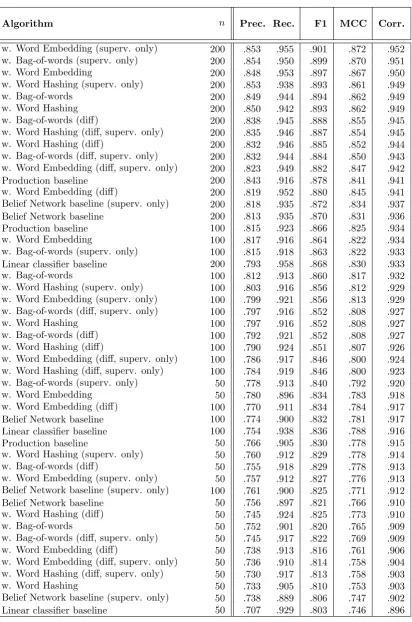
5.2 K-fold evaluation results of the matching algorithms on dataset C. . . 31

5.3 K-fold evaluation results of the indexing algorithms on dataset R. . . 32

5.4 K-fold evaluation results of the indexing algorithms on dataset C. . . 33

A.1 Significance levels of the matching algorithms on dataset R. . . 44

A.2 Significance levels of the matching algorithms on dataset C. . . 45

A.3 Significance levels of the indexing algorithms on dataset R. . . 46

A.4 Significance levels of the indexing algorithms on dataset C. . . 47

B.1 Training set evaluation results of the matching algorithms on dataset R. . . 50

B.2 Training set evaluation results of the matching algorithms on dataset C. . . 51

B.3 Training set evaluation results of the indexing algorithms on dataset R. . . 52

B.4 Training set evaluation results of the indexing algorithms on dataset C. . . 53

(8)

(9)

1

Introduction

Modern organizations maintain large databases as a result of their core business. A key part of the data inside these databases, especially in the service industry, will consist of contact data. Organizations have to track the contact information of their suppliers, employees and customers. Over many years, these databases have gathered many duplicate entries. For example, internal departments might move to a single database system and organizations can be bought or merged. Finding and solving these duplicate entries helps organizations to be both more effective and more efficient. However, finding duplicate entries is not always straightforward. Because of the fuzzy nature of contact data, duplicate entries of the same contact will likely differ slightly. Both names and addresses are subject to many variations: one entry might contain an initial and the other the entire given name. Phone numbers and email addresses are often more easily standardized, but might not always be present.

While the problem of duplicate detection1 is not always straightforward, there are numerous techniques that give good results. A typical approach is to calculate a number of string distance measures between the different fields of the two records and use these distances to determine whether two records are duplicate or not. Historically, doing so involved domain experts skillfully creating matching rules, but today it is more common to derive these rules using machine learning techniques.

Typically the machine learning algorithms used to create these matching rules are supervised algorithms, meaning that they require annotated data to train on. Models created by supervised algorithms have the potential of producing high-quality results, but large sets of labeled data are required to do so. The creation of labeled data is time consuming as a domain expert has to manually classify pairs as either duplicate or non-duplicate.

A potential solution to reduce the dependency on labeled data is provided by recent advances in deep learning. In semi-supervised learning, such as certain deep learning techniques, not only the

1_{The problem of duplicate detection is also referred to as record linkage, entity resolution, merge/purge or}

identity resolution.

(10)

2 CHAPTER 1. INTRODUCTION

labeled data is used for training, but also the unlabeled data. An example of a semi-supervised deep learning technique is a deep belief network.

Using unlabeled data in addition to labeled has the potential to achieve comparable results with less labeled data, as large amounts of unlabeled data take the place of some of the labeled data. Replacing the role of labeled data with unlabeled data will reduce the human effort required to train models: because in contrast to labeled data, unlabeled data is easily available in the form of the dataset to be processed.

1.1 Research questions

The goal of the proposed research is to investigate the effects of deep learning, and specifically deep belief networks, when applied to the problem of duplicate detection. Being semi-supervised, deep belief networks can make use of both labeled and unlabeled data. The expectation is that this allows for more advanced models than traditional machine learning techniques, which can only make use of labeled data. The following research questions will be addressed:

Research question 1 How does the use of unlabeled data in addition to labeled data influence duplicate detection quality?

The main question that this research aims to answer is about the influence of unlabeled data in addition to the labeled data. To make semi-supervised training possible, a belief network is used for matching. Using unlabeled data is expected to improve the performance of the model and increase the quality of the matching results, especially as the amount of labeled data gets lower. Research question 2 How does the use of layers such as auto-encoders to create a belief network influence duplicate detection quality?

While deep belief networks offer the possibility of training networks in a semi-supervised way, they make certain requirements on the structure of the neural network, for example the use of auto-encoder layers. By evaluating these changes separately, it becomes possible to distinguish between the effect of the added unlabeled data and the required structural changes.

Research question 3 How does the use of other techniques commonly used in natural language processing with deep learning, such as word embedding and semantic hashing, influence duplicate detection quality?

(11)

2

Background

The algorithms described in this paper employ a number of machine learning techniques. This chapter aims to give a short overview of some of the basic techniques and concepts in machine learning. While these techniques are described in general terms, the focus is on those relevant to this research. Those who are already familiar with these techniques could consider skipping this chapter and going to Chapter 3, where related work is discussed in relation with this research.

2.1 Machine learning

Machine learning is the study of algorithms that can learn from and make predictions on data. These algorithms build models from examples, rather than following strictly static instructions. Not only are several of these models capable of higher accuracy than manually created models, they are also capable of adapting to new circumstances without intervention as both model creation and evaluation can be automated. It is therefore not surprising to see machine learning algorithms being adopted in a variety of scenarios.

There are a lot of different machine learning algorithms and they are typically placed in several different categories, based on which kind of problems they are suitable for. For example, machine learning algorithms are categorized as either supervised or unsupervised, depending on whether or not the algorithm requires the data to be annotated with a target value. Although uncommon, there are also algorithms that strictly do not fall under either supervised or unsupervised learning: semi-supervised algorithms, for example, are capable of using both labeled and unlabeled data. Within supervised learning, a distinction is usually made between classification and regression. In classification the target value is one of a fixed set of values. This type of value is more commonly known as an enumeration in other fields of computer science. For example, an email filtering system would classify new mails as either spam or non-spam. In regression the target value is

(12)

4 CHAPTER 2. BACKGROUND

numeric. Classification and regression machine learning algorithms are referred to as respectively classifiers or regressors.

2.1.1 Evaluation of classifiers

The evaluation of different classifiers plays a large role in the application of machine learning. During the evaluation, different classifiers are compared to each other and to trivial baselines. An evaluation of a number of classifiers consists of several key elements. The different classifiers are trained on the data and the resulting models are in turn applied to the data. Finally the output is compared to the golden standard and the results of the comparison are summarized using some metric, for example error count. The results of the comparison give insight in which classifiers are better suited to a certain problems, and if a classifier is an improvement over baseline solutions at all.

A typical evaluation is more complicated than simply training on the whole dataset and looking at the results. This kind of evaluation is known as thetraining set evaluation, as the model is evaluated on the same data it is trained on. The training set evaluation is not typically used to compare classifiers against each other. The most important reason is that training set evaluation does not properly reflect the generalization error of a classifier, or how a classifier performs on unseen data.

The limitations of the training set evaluation can be illustrated by the nearest neighbour classifier. Unlike most classifiers, this classifier does not create a model of the input upon training. The entire training set is simply stored in memory. When classifying, the nearest neighbour classifier [8] looks for the training sample nearest to the input, and outputs the class of that sample. During a training set evaluation, the training sample closest to the input is simply the input itself, resulting in the illusion of a zero error rate1_.

Error metrics

In practice errors are not directly combined into a error metric. The results are first summarized in aconfusion matrix. A confusion matrix is a matrix in which the rows represent the true classes and the columns represent the classes predicted by the model. In case of only two classes, the confusion matrix is a two-by-two matrix. Each cell in the matrix contains the number of samples that belong to a certain class and have been classified as a certain class. This includes samples that have been classified as the actual class.

Another difference in practice is the used error metric. The error rate or related metrics such as the percentage of samples classified correctly are problematic in certain scenarios, for example when the distribution between the classes is skewed. In the case of duplicate detection, classifying pairs as either duplicate or non-duplicate, the odds are heavily skewed towards two random records being non-duplicate. In such a scenario, a classifier that always returns the majority class will have a very low error rate.

In practice it is relevant to find instances of the rare class between many cases of the common class. In these cases other evaluation metrics, such as precision and recall, are typically used. Precision is defined as the part of retrieved elements that is relevant, while recall is the part of

1_{In case the training set contains multiple entries that are completely equals except for the target value, the}

(13)

2.1. MACHINE LEARNING 5

the relevant elements that have been retrieved. As most problems require a balance between both precision and recall, they are commonly combined in the F1-score.

Another error metric that is commonly used is theMatthews correlation coefficient (MCC) [37]. Like precision and recall, the MCC takes the distribution of the classes into account. An advantage of MCC over these other metrics is that MCC uses the number of true negatives, which precision and recall do not. The MCC also does not differentiate between a desirable class and a undesirable class. When using precision and recall selecting a certain class as desirable could create a bias [45]. Similar to the F1-score, the MCC is the combination of two error metrics known as informedness and markedness.

MCC = _√ T P ×T N−F P×F N

(T P +F P)(T P +F N)(T N+F P)(T N+F N) (2.1)

K-fold evaluation

A training set evaluation does give not give good insight in the generalization error, but there are other evaluation techniques that do. In general, these evaluation techniques focus on evaluating the classifier on data different from the data that it is trained on. A common technique that does this is called a K-fold evaluation [54].

In a K-fold evaluation the available data is split in K parts. Each of the K parts is referred to as a fold, hence the name K-fold. In each round of the evaluation, one of the folds is set aside for evaluation. The algorithms are trained on the other folds and then evaluated on the fold that has been set aside for evaluation. This process is repeated so that each fold is used in evaluation once.

2.1.2 Genetic algorithms

Genetic algorithms are a flexible machine learning technique inspired by natural selection. Initially a population of random candidates is created. Every cycle of the genetic algorithm all candidates in this population are evaluated using some metric. A selection is then made of the higher scoring candidates, from which the population for the next generation is generated. There are different ways for generating this next generation: existing candidates can be mutated, two candidates can be combined using cross-over and a small number of new random candidates can be introduced. After a number of cycles the population will start to consist of better performing candidates than the initial population. Eventually the best performing candidate is picked from the population. If the metric used to evaluate the population is static, the genetic algorithm will result in a solution that is optimized for the used metric, but performs worse on closely related evaluations. For example, if the used metric evaluates on basis of a set of labeled training samples, the solution might have good results on this set, but generalizes badly to new data. To prevent overfitting in the genetic algorithm, a common approach is to only use part of the labeled training set in the evaluation each generation [20]. This way all candidates in the same generation are evaluated on the same training data selection, to ensure a fair comparison, but the selection changes with every generation.

(14)

[image:14.595.234.400.97.316.2]

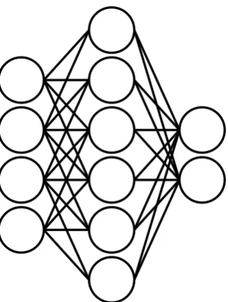
Figure 2.1: Neural networks are networks of neurons, which are arranged in layers. Input values are propagated through the network.

2.1.3 Neural networks

Neural networks are a type of classifiers based loosely on the working of the human neural system. A neural network (see Figure 2.1) is a network of neurons, which are typically arranged in layers. With exception of the input layer, each layer of neurons takes the output of the previous layer and processes it further. During the processing, each neuron calculates the weighted sum of outputs of the previous layer and transforms it using an activation function. Typically the weighted sum also includes a bias value, which is added regardless of input values. Although each neuron in a layer uses the same input, the weights are different for the different neurons, resulting in different outputs.

There are a wide variety of neural network configurations, with either a different network structure or different activation functions. It is also possible to combine different activation functions in the same network. For example, when performing regression, it is common to replace the activation function of the output layer with the identity function to create a simple weighted sum. A single neuron with the identity activation function is conceptually identical to a linear regression model.

2.2 Deep learning

Deep learning is the term used for algorithms used within machine learning that focus on learning higher level abstractions. By learning higher level abstractions, these models tend to perform significantly better on a number of tasks that traditionally were considered difficult in machine learning, such as image recognition.

(15)

2.2. DEEP LEARNING 7

might be edge detection, some kind of shape indication, color information and some description of the texture. Because not every set of features is equally good, a lot of time in machine learning is spent on optimizing the features to train on. As deep learning is capable of learning higher level abstractions, these features do not need to be constructed manually, but can instead be learned. By learning higher level features there are a number of advantages. First of all, automatically learning features saves the time that would otherwise go into designing these features. Secondly, features created by deep learning are often better than hand-made features. There are a number of underlying reasons for this: errors in the network can be back-propagated into the features, and features learned this way are specific to the problem at hand.

2.2.1 Deep neural networks

A deep forward neural network is the deep variant of the common shallow feedforward neural network. A deep forward neural network consists of an input layer, multiple hidden layers and an output layer. Connections only exist in one direction: from the input layers through the hidden layers to the output layer.

Where shallow neural network rely mostly on backpropagation for training, in networks with more layers there are a number of problems that result in only using backpropagation not being practical [19]. A common solution is to pretrain the layers in the network. While there are different ways of pretraining, a common technique is to treat all layers as either auto-encoders or restricted Boltzmann machines. The layers can then be trained one layer at the time. This process avoids the problems that occur when using only backpropagation on a large number of layers. Networks of this type are called deep belief networks. After the pretraining the full network is further optimized using backpropagation.

In addition to pretraining there are a number of other techniques that intend to make very large deep neural networks more feasible. Most of these are not only applicable to feedforward neural networks, but also to the other variants.

One of the noticeable changes is the use of a different activation function. Where traditional neural networks often employed sigmoid or tanh function, recently the use of therectified linear unit (ReLU) [43] has become more popular [34]. The ReLU function, f(x) =max(0, x), returns the input value, except when this input value goes below some threshold, in which case the threshold is returned. While a relatively simple function, it is capable of providing the same kind of non-linearity as the other activation functions. Due to its simplicity, the ReLU function is cheap to compute. As an additional advantage, it also creates a lot of zero values, which simplify further calculation even further.

Another new activation function is themaxout function [21]. The output of the maxout function is defined as the maximum values of all weighted input values. Maxout networks can be used to represent any kind of function. The advantages of maxout are similar to those of the ReLU function.

Deep belief networks

(16)

belief networks, also known as Bayesian networks. Like Bayesian networks, deep belief networks model dependencies among the input variables.

The important difference between deep belief networks and normal deep neural networks is the way the training is done. Deep belief networks are pre-trained in an unsupervised fashion on unlabeled data to create a model of the dependencies among the input variables. This is done by training each layer on top of the underlying layer, with each layer improving the overall representation of the data. The higher level representation can then be used as the input to a output layer, like those in neural networks.

[image:16.595.152.484.310.535.2]

After the pretraining, deep belief networks are further trained using the same supervised algorithms used for deep neural networks. Both approaches can also be combined in a semi-supervised approach, by first training on unlabeled data and then finalizing using labeled data. This allows for networks that are based on both labeled and unlabeled data. Aside from the avoiding the problems normally related with training a large network using backpropagation, the ability of semi-supervised learning is another advantage of deep belief networks over regular deep neural networks.

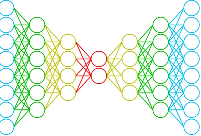
Figure 2.2: A deep auto-encoder is a deep neural network consisting of a number of layers. Characteristic of auto-encoders is the size of the layers: the layer sizes are symmetrical and the closer to the middle, the smaller the layers get.

2.2.2 Auto-encoder

(17)

[image:17.595.112.452.91.273.2]

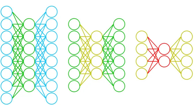
Figure 2.3: A deep auto-encoder can be efficiently trained layer-by-layer by viewing every layer as a small auto-encoder. For the auto-encoder in Figure 2.2, this process combines down to training the above three networks, each time using the previous layers as preprocessing for the next.

In addition, auto-encoders do not require labeled data and are therefore an unsupervised machine learning algorithm. The same data is used as both input and output.

Auto-encoders can occur in both shallow variants, with one hidden layer, and deep variants, with more than one hidden layer. Training of a deep auto-encoder only through the use of backpropagation results in similar problems as with regular deep neural networks. For this reason deep auto-encoders are typically deep belief networks and use the corresponding pretraining technique.

One of the ways to pretrain a deep auto-encoder, and deep belief networks in general, is to view each layer as a shallow auto-encoder. This shallow auto-encoder can then be training using normal techniques. An example of this process is shown in Figure 2.3.

Semantic hashing

Semantic hashing [48] is a technique used to create an index of all documents in such a way that similar documents can easily be retrieved. In semantic hashing the compact code of an auto-encoder network is used for this purpose. Ideally all similar documents have the same compact code. During the training of the auto-encoder network a large amount of noise is added. After training, the compact code is created from the activations in the bottleneck layer of the auto-encoder network. This compact code is converted to binary by applying a threshold. Notice that in [48] the threshold used is close to zero, due to most of the values being closer to zero than one.

2.2.3 Applications

(18)

Speech recognition

Speech recognition is the area of research in which the aim is to understand spoken language. A subtask of spoken language understanding is transforming speech to text in an automated fashion. A typical application of speech recognition is in voice controlled user interfaces, for which speech recognition forms an essential part. For a long time, the best performing model for this problem was the hidden Markov model [12]. Several comparisons with traditional neural networks have been made, but the results were not as good as the hidden Markov model [42]. The results of the hidden Markov model were however improved upon with the application of deep learning. Early results using a deep neural network show already substantial improvements [9]. Later models use deep recurrent neural networks in combination long short-term memory units to improve performance even further [22].

Speech synthesis

Speech synthesis is the area of generating speech from text, giving roughly the inverse operation of speech recognition. As with speech recognition, speech synthesis has traditionally been done using hidden Markov models, as well as a number of other techniques. Several deep learning based models have been shown to improve the generated speech. For example, by using a deep belief network as a generative model for speech [28, 36]. In [56] a discriminative deep neural network is used instead, trained to predict the probably distribution normally produced by the hidden Markov model. In [16] a deep neural network is first used to create a compressed version of the generated speech. The compressed speech is then used in second stage to generate final output.

Image recognition

Image recognition is a wider area of research, consisting recognizing objects in images. Early work on deep learning already looked into replacing the previously commonly used principal components analysis with a deep auto-encoder [25]. Deep learning has also been used to improve upon state of the art in different image benchmarks, for example [47] using large convolutional neural networks [31]. Another possibility is the use of a large amount of sparse auto-encoders to allow semi-supervised training [32].

Image recognition has also been used in multi-modal systems. A multi-model system is one where data comes multiple input channels. An example would be converting an image to tags [53]. This is done by creating a deep restricted Boltzmann machine that combines input from both images and text, after two sets several layers solely focused on only one but not the other. More recent works are capable of generating full sentence captions for a given image [55].

Information retrieval

(19)

done using a deep neural network, but with the use labeled data. A deep stacking network is used in [11], where it is trained in such a way to optimize the ranking of suggested documents.

Natural language processing

Natural language processing is concerned with the processing of natural language. Typical tasks within natural language processing include parsing, part-of-speech tagging, but also higher level problems like machine translation. In [6] a convolutional deep belief network is used to performing many tasks that are traditionally done by different algorithms, such as tagging and chunking. In [5] parsing is done using a deep recurrent convolutional architecture. In [7] a minimal set of predefined features is used, in an attempt to create a model that is as language independent as possible. The internal representation is learned from unlabeled data.

In [51] a recursive neural network is used to create a nested tree structure which can be used for parsing. In [52] a similar nested structure is used for sentiment analysis.

One of the major recent improvements in natural language processing is the use ofword embedding [6, 7]. Word embedding is a technique in which every word has a corresponding vector it can be mapped to. This vector mapping is constructed in such a way that it aims to represent the context of a given word. The result is that words that occur in similar contexts have very similar vector representations. This is useful because the context of a word contains a lot of information about a given word and its meaning that cannot be extracted from the word itself. For example, the words ’cat’ and ’dog’ do not have a single letter in common, but both represent animals that are four-legged, pets, etc. Word embedding models can be trained using a number of different algorithms, including neural networks.

Word embedding has been applied to many languages. For use in machine translation word embedding has also been extended to two languages at the same time [57]. This requires additional restrictions to ensure that the word embedding mappings in both languages are compatible. In [18] two language word embedding is also used, augmented with a deep neural network.

(20)

(21)

3

Related Work

The different algorithms used in the evaluation described in Chapter 4 are not new, but originated in related works of research. This chapter aims to give a description of those algorithms. In contrast to Chapter 2, which explains the basic concepts, the algorithms described here that are either used in the evaluation, or closely related to those used in the evaluation.

3.1 Duplicate detection

Duplicate detection is not a new area of research. A lot of previous works, both academic and commercial, investigated different techniques to improve the quality and performance of a duplicate detection system.

The core step in every duplicate detection system is to compare records against each other to determine if they are duplicate records or not. This matching of records is usually in a pair-wise fashion. By comparing the records pair-wise, the pair and the differences can be evaluated in depth. If two records are determined to be duplicate records, they are typically given a score and stored for further reference.

Because of the pair-wise comparison, this matching approach grows quadratic with the number of records. As a result, naively comparing every record with every other record is very time costly on larger datasets. Most duplicate systems therefore use an indexing step. This indexing step aims to reduce the number of evaluations, allowing duplicate detection to remain practical on larger datasets.

Notice that in some situations either the indexing or matching step is left out. If indexing manages to produce high quality results, or the quality requirements are not too high, only using an indexing step will be sufficient. Conceptually this is identical to having a matching phase that classifies all pairs as duplicate. Likewise, on some small datasets indexing might not be needed. The matching phase will then compare every record to every other record.

(22)

14 CHAPTER 3. RELATED WORK

3.1.1 Matching

In the matching phase records are compared in a pair-wise fashion. This allows for an advanced comparison between two records. This is essentially a classification problem: a pair has to be classified as either duplicate or non-duplicate based on the contents of the records. The approach is typically to calculate a set of features between the fields of the two records. This approach is used not only common in machine learning based systems, but also in systems in which domain experts provide the logic for determining the outcome.

Whereas models configured by domain experts usually stick to more easily understandable models such as decision trees and linear regression, models trained by machine learning can be more complex. Examples of such more complex algorithms are neural networks and support vector machines. In practice the difference in accuracy between different classifiers is relatively small given the same features (5-6% error rate on one dataset, 13-14% on another) [30]. As the different algorithms are functionally interchangeable, some frameworks also allow for the classifier to be changed through configuration [29].

Matching features

The matching phase employs a number of features to determine if two records refer to the same entity. This is more practical than trying to work on the string values directly. As matching is done in a pair-wise comparison, the features are comparisons between the different fields of the two records. Every of the features described below will typically be applied to each field. Basic features include equals checks or empty checks. String edit distances are also commonly used as features, as they are capable of handling small errors. With string edit distances the output is a measurement of similarity for the two strings. There are many different string edit distances that have been proposed over the years, the list below includes only a small selection. In practice matching algorithms do not need features for many edit distances, as there is a large overlap between the types of string differences covered by the different edit distances.

• The Jaccard index is used mostly in statistics for comparing similarity and diversity of two sets, calculated by dividing the size of the intersection of two sets by the size of the union of these sets. For string comparison this means that both words will be seen as two sets of letters and the order of these letters isn’t taken in consideration. This metric is easy to calculate and mostly strong in identifying two completely different strings, meaning two words that don’t have many of the same letters in them [23].

• The Jaro distance is a measure of similarity between strings, mostly used for duplicate detection, which scores between 0 (no similarity) and 1 (exact match), intended primarily for short strings. It is based on the number and order of the characters two words share. In record linkage, good results have been obtained using this method or variants of it, in both effectiveness and efficiency [4].

• Levenshtein is the most well-known string distance metric, also often referred to specifically as the string edit distance. It is used mostly in natural language processing and allows for three operations to make one string into another: insertion, deletion and substitution which all have a cost of 1 [35].

(23)

3.1. DUPLICATE DETECTION 15

features involves doing an additional pass of the data to gather all the required statistics. Other candidates for features are phonetic algorithms as they allow comparing of two strings that are not exactly equal. As with the string edit distances, there is a lot of overlap between the different phonetic algorithms.

These features can be applied on entire strings, but can also be applied on the different tokens within a string. Thelevel 2 score is calculated by splitting the string in tokens and recursively applying the distance feature to the different tokens. The scores on the different tokens are combined using the formula shown in Formula 3.1.

score(A, B) = 1 k

An

∑

i=0

maxBn

j=0

(

score(Ai, Bj) )

(3.1)

Some distances, such as the Monge-Elkan edit distance, already calculate the score on a per token basis internally [41].

3.1.2 Indexing

Performing some sort of indexing is an often necessary optimization step. Comparing every database entry against every other entry is not feasible on databases that can contain hundreds of millions of records. By performing an indexing step the number of pairs that have to be evaluated is reduced. Most practical implementations of duplicate detection systems therefore perform such an indexing prior to comparing records to each other [3].

There are different techniques to reduce the number of comparisons that need to be done in matching. All of these do so by placing some kind of restriction on the duplicates that can be found by the system. The kind of restriction depends on the applied algorithm and its parameters. As with matching, the indexing has to find a balance between precision and recall. Indexing techniques are mostly focused on recall, but too many candidate pairs have an impact on the speed of the system. While this is a problem in production systems, this might not always be a problem in academic settings. In some scenarios it is even feasible to not include any form of indexing.

Blocking

Blocking [15] is widely used as an indexing technique as it provides a good balance between precision and recall. In blocking, the number of pairs to be evaluated by matching is reduced by dividing the records in a number of blocks. Only records within the same block are compared by matching. Records are typically part of multiple groups as a means to introduce redundancy. Another way to implement blocking is to calculate several hashes for each record. Two records are only compared if there is at least one common hash. This can be efficiently implemented using a hash map, by checking which two records generate a hash collision.

(24)

16 CHAPTER 3. RELATED WORK

depends on the used training algorithm. For blocking systems the typical choice is by far the genetic algorithm, as this tends to result in good configuration values [14, 27].

Also not surprising, indexing techniques, such as blocking, are more restricted in terms of matching quality than matching algorithms. In [27] a F1-score for blocking is reported of 0.42 for one dataset and 0.68 for another. In [3] the F1-score results for blocking are between 0.5 and 0.6 for two of the four datasets, and below 0.1 for the other two. In [14] recall scores are reported between 0.84 and 0.93 for the three datasets.

There are several different algorithms described in literature to automatically determine the near-optimal blocking hashes. There are both supervised and unsupervised algorithms. The supervised algorithms require an annotated sample to generate the blocking hash. The unsupervised variants, on the other hand, do not require annotated data but place several assumptions on the dataset [44].

A common method to generate the blocking hash functions is with the use of a genetic algorithm. The genetic algorithm method takes an incremental and greedy approach when it comes to finding multiple hashes [10, 38]. The algorithm will first try to find the single best hash according to the specified metric. The covered duplicate pairs are then removed from the training set, and the algorithm will try to find the single best hash on this new set. This process continues until all duplicate pairs are covered or additional hashes no longer improve the overall metric. This incremental process is called the Sequential Covering Algorithm [40] and is used in several indexing algorithms.

3.2 Natural language processing with deep learning

While the application of deep learning to duplicate detection on textual data seems to be novel, there is a lot of existing work that covers the processing of textual data. Within the field of natural language processing, deep learning recently has been applied to many aspects with great success.

3.2.1 Semantic hashing

(25)

3.2. NATURAL LANGUAGE PROCESSING WITH DEEP LEARNING 17

addition to the unlabeled data increases the NDCG@10 (Normalized Discounted Cumulative Gain) from 0.459 to 0.486 for use in information retrieval systems.

Another technique, also presented in [26], is word hashing. In word hashing sets of n-grams are used to represent words. Doing so increases the NDCG@10 even further, to a reported 0.494. As the number of n-grams is smaller than the number of words, this approach requires less input features than a bag-of-words approach. Word embedding is less complex than word embedding and does not represent the context of word. An additional advantage is that morphological variations are mapped to similar n-grams, making word hashing capable of doing stemming operations.

3.2.2 Word embedding

Another area that is related to duplicate detection of textual data is natural language processing. One of the important recent developments in natural language processing is word embedding. Traditionally words are encoded by an arbitrary index: the word with index four is then represented by a list of features in which the fourth feature is one and everything else zero. Longer sequences can be represented as a bag-of-words or by concatenating the word feature in order. Both ways of encoding result in a number of features equal or larger than the dictionary size, which is usually very large in most scenarios. The underlying reason is that such encoding does not carry a lot of information. These encodings also have difficulty dealing with words unseen in the training data. Word embedding instead chooses to represent word as vectors in a low dimensional, continuous space, preferably with some meaningful dimensions. There are different algorithms in use to generate this meaningful encodings. Usually these algorithms are trained on large sets of unlabeled data, such as the entire Wikipedia corpus. Common algorithms are neural networks but also different kinds of principle component analysis, such as for example in [33].

(26)

(27)

4

Methodology

Each of the research questions implies the comparison of different variants. For example, the main research question, research question 1, is about the effect of additional unlabeled data. To answer this question two variants have to be compared, one of which uses semi-supervised learning to make use of unlabeled data. In same way, the approach to answer the other research questions listed in Chapter 1 is to compare the different algorithm variants against each other on different datasets. This chapter describes the evaluation methodology, how the evaluation is conducted, with the intention of making the results reproducible.

4.1 Evaluation setup

The evaluation consists of an indexing evaluation and a matching evaluation. The setup of both evaluations is largely the same for simplicity. Aspects in which both evaluations differ will be mentioned.

During the training of the different algorithms both labeled and unlabeled data are available. The evaluation is restricted to the part of the dataset that have been manually classified as either duplicate or non-duplicate. As the unlabeled data does not contain labels, it cannot be used during the evaluation phase.

4.1.1 K-fold

The different algorithms are evaluated on the datasets using an K-fold evaluation. In a K-fold evaluation the dataset is partitioned in K distinct folds. In each round the algorithm is trained on all but one of these parts and then evaluated on the part that has been left out. This gives a better approximation of how well the algorithms perform on unseen data. The evaluation on each left out fold results in K confusion matrices. These confusion matrices are summed to create

(28)

20 CHAPTER 4. METHODOLOGY

one overall confusion matrix, which is used for calculation of the error metrics. This process introduces less bias than calculating an error metric for each fold separately and then taking the average [17].

The experiment uses a K-fold evaluation with just 2 folds. Using a higher number of folds will increase the number of training data potentially available to the algorithms. For example, when using a more typical 10 folds, the algorithm would have access to 90% of all labeled data during each training run, compared to 50% with 2 folds. However, as the evaluation is focused on small training sets, the amount of available training data is already artificially limited. Having more folds also reduces the number of labeled pairs still together in the testing fold: if one of the two records in the pair is not in the fold, the pair is incomplete and disappears.

To minimize the influence of the exact distribution of the folds and training data selection, the process of randomly creating the folds and performing the K-fold evaluation is repeated 5 times. This kind of evaluation is known as the 5x2 cross-validation [1]. Repeating the 2-fold more than five times no longer gives new information as the repetitions become too dependent [13]. All the indexing algorithms are evaluated on exactly the same folds, as well as all matching algorithms. No special measures are taken to ensure the folds are kept completely identical between the indexing and matching evaluation.

The classifiers will also be evaluated on the training set to determine if the algorithms are overfitting or underfitting. When determining the best algorithms the results on the training set will not be considered. In the training set evaluation the amount of test data varies between variants, as the different variants will be provided with different amounts of training data.

Distribution of pairs and records over folds

The creation of the folds involves distributing both pairs, for supervised training, and records, for unsupervised training, over the folds. Both categories cannot be simply distributed independently: pairs have to be discarded when both records related to the pairs are not in the same fold. It follows that the probability of this occurring increases as the number of folds increase.

To soften this issue, the pairs are distributed over the folds first. The records are then distributed over the folds according to the pairs they are related to. The remaining records, those that are not linked to any marked pair, will be distributed randomly to be used as unlabeled data. As some records are linked to in multiple pairs, some records might risk ending up in more than one fold. In this case, the record is assigned to only one of the folds. Assigning a record to multiple folds would result in the possibility of leaking of information from the evaluation data to the training data.

4.1.2 Training set sizes

For each algorithm there will be variants which discard part of the labeled training data, resulting in variants with a different number of training samples. These variants can then be compared against each other, to determine the effect of the training sample size. The part of the training data to discard is selected randomly. Labeled data that has been discarded will stay available to the algorithm as unlabeled data, in addition to the already existing unlabeled data.

(29)

4.2. MATCHING VARIATIONS 21

to compare the algorithms with 50, 100 and 200 labeled training set samples for each of the two classes, duplicate and non-duplicate.

Some of the algorithms listed below also make use of unlabeled data. For these algorithms unlabeled data is available. Unlike the labeled training data, there are no artificial limits on the number of samples. For practical reasons however, unlabeled data was restricted to 10000 samples (or less) in algorithm implementation.

4.1.3 Error metrics

During the evaluation the metrics precision, recall, F1-score, Matthews correlation coefficient (MCC) and correctness rate will be measured and reported. These error metrics will be used for

comparing the different algorithms.

Notice that while for the indexing evaluation recall is considered more important in practice than precision, no such preference applied during the evaluation. The assumption is that algorithms capable of optimizing for balanced precision and recall are also capable of optimizing for recall, as optimizing purely on recall is easier in theory1_.

4.1.4 Significance checking

In addition to measuring error metrics, data is also collected on the significance of the differences between the different algorithms. The significance check is performed using a binomial test [49]. In order to calculate the significance of the difference in performance between two variants all samples that both classified identically are first discarded. The remaining samples are samples A got wrong and B got right, and samples A got right and B got wrong. These differing samples are interpreted as a series of Bernoulli-trials. The p-value for the two algorithms can be calculated using the binomial distribution. The resulting values will be corrected using the Holm-Bonferroni method to adjust the fact that multiple significance checks are performed for all the different variants.

4.2 Matching variations

The first part of the evaluation covers pair-wise matching. To determine the effect of the different matching algorithms the variants are compared against each other. The hyperparameters of each of the different variants are determined using the tuning set (see Section 4.4).

4.2.1 Production matching

The production matching is the matching algorithm used by a commercial company in their latest duplicate detection engine. As this is part of proprietary software, the specific implementations details are not known. In addition, while the other variants are tuned towards a high MCC, this is not the case for the production matching algorithm.

1_{The theoretically best indexing technique in terms of recall is no indexing at all, simply comparing every}

(30)

4.2.2 Linear classifier

A linear classifier is used as a baseline for the matching evaluation. The reason to use a linear classifier is that while a linear classifier has only limited processing capabilities, the input features are already very high-level. In addition, a linear classifier is comparable to the production implementation.

This linear classifier does not work on the string values directly, but instead use a set of features. For each pair to be matched we calculated a set of string distance metrics between the different columns of the two records. These metrics are calculated separately for each of the columns. The result is a feature space of around a hundred numerical features. This feature space also consists of features which indicate anomalies like empty columns. Working with these features is more practical than the original feature space of around ten string features.

For practical reasons the linear classifier is implemented as a neural network containing only a single neuron, which is conceptually identical to a linear classifier. The hyperparameters have been set at 1000 iterations and a learning rate of 0.010, as determined on the tuning set.

4.2.3 Deep learning-based matching

The matching based on deep learning consists of multiple variants. The evaluation is not only to compare traditional matching techniques against deep learning, but also to evaluate multiple deep learning variants and see which technique works best for matching.

Variant Features Encoding

Semi-supervised

Belief Network baseline - - semi-supervised

w. Bag-of-words bag-of-words both, unmodified semi-supervised

w. Word Hashing word hashing both, unmodified semi-supervised

w. Word Embedding word embedding both, unmodified semi-supervised w. Bag-of-words (diff) bag-of-words abs. difference semi-supervised w. Word Hashing (diff) word hashing abs. difference semi-supervised w. Word Embedding (diff) word embedding abs. difference semi-supervised

Belief Network baseline (superv. only) - - supervised only

[image:30.595.89.546.395.613.2]

w. Bag-of-words (superv. only) bag-of-words both, unmodified supervised only w. Word Hashing (superv. only) word hashing both, unmodified supervised only w. Word Embedding (superv. only) word embedding both, unmodified supervised only w. Bag-of-words (diff, superv. only) bag-of-words abs. difference supervised only w. Word Hashing (diff, superv. only) word hashing abs. difference supervised only w. Word Embedding (diff, superv. only) word embedding abs. difference supervised only

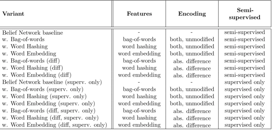
Table 4.1: Overview of the deep learning based matching algorithm variants.

The table indicates for each variant which additional features (in addition to the base features) are included, how the additional features are encoded and how the variant is trained.

(31)

4.2. MATCHING VARIATIONS 23

every record. Regardless of word encoding technique, the encoding is applied on only one word at the time. In fields that contain multiple words, the field will be split and the word encoding technique will be applied independently to each of the words in this field. This process is repeated for every field in the record.

As the number of words can vary between different records, a fixed maximum length is set. Values with contain more words than this maximum number are cropped. The maximum length is set in such a way that this is a rare event. Shorter values are padded with a special padding word. Again, this process is used regardless of word encoding technique.

The resulting representation will be provided to the deep belief network. As matching involves two records, the features of the deep belief network includes the representations of both of these two records. In addition to the representations of these two words, the edit distance features that are already present in the belief network baseline are also included.

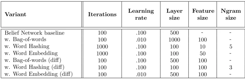
The hyperparameters for all variants have been optimized using the tuning set. For each of the variants the highest performing configuration of hyperparameters has been selected for use the evaluation. The overview of selected hyperparameters can be found in Table 4.2.

Variant Iterations Learning rate

Layer size

Feature size

Ngram size

Belief Network baseline 100 .100 500 -

-w. Bag-of-words 100 .010 1000 100

-w. Word Hashing 1000 .100 100 10 5

w. Word Embedding 1000 .100 100 50

-w. Bag-of-words (diff) 100 .100 500 100

-w. Word Hashing (diff) 100 .100 100 100 3

w. Word Embedding (diff) 100 .010 500 100

-Table 4.2: Overview of the hyperparameter configuration for each of the matching variants The supervised only variants use the same hyperparameter configuration as the corresponding semi-supervised variant. Layer size indicates the size of the hidden layer. Feature size indicates the number of additional inputs in the network per token in the record.

Difference calculation

Instead of providing the word representations of both records separately, it is also possible to provide the difference between both. This makes the new features conceptually a lot closer to the edit distance metrics, which are common in matching, as discussed in Chapter 3. For example, the baseline matching algorithms also use several edit distance features.

This difference calculation variant replaces the features of both records by a new set of features, namely the absolute difference between the two records. This difference is calculated separately for each feature. As both records use the same word encoding techniques this features should be roughly comparable.

[image:31.595.70.488.308.444.2]

(32)

word of one record is compared against the first word in the other record, the second word to the second word, etc. To handle this case, the difference calculation provides features not just between one word and the word at same position in the other record, but also between a word and all other words in that field.

Bag-of-words

The baseline word encoding technique used during the evaluation is bag-of-words. While simple to implement, bag-of-words has long been used for the representation of words.

In bag-of-words a collection of words is represented by a vector where the value at each index indicates the frequency of the corresponding word. The precise mapping of indexes to words is based on the vocabulary.

As the two other word encoding techniques are applied on word level, this approach was also taken for the bag-of-words implementation. This means that every word in every field has its own bag-of-words vector, and each of these bags-of-words cover only one word. In other words, the values in the vector will be zero everywhere, except for the value at the index of the word that is being represented.

Word hashing

Word hashing [26] is a technique in which the N-grams of a word are used to represent a word. The advantage of this over a normal bag-of-words is that textually similar words are grouped together. For example, the presentation of ‘arguments’ and ‘argument’ will be very similar. The idea behind word hashing is roughly comparable to that of stemming.

In the word hashing variants all words are represented as a collection of short substrings of a few characters. These character N-grams are then represented using a bag-of-words encoding, but with every value indicating the presence of a N-gram instead of a word. Like in bag-of-words, the result will be a vector where the value at every index will indicate the frequency of the corresponding N-gram. For simplicity frequencies are restricted to either non-zero or zero. For the N-grams encoding N-grams with length 3 are used, which are also known as trigrams. Notice that the N-grams are on character level, so each trigram will be a string of 3 characters. The start and end of a word are explicitly modeled, by padding words with a padding character before converting to N-grams. So for example ‘word’ would result in the N-gram ‘ wo’, ‘wor’, ‘ord’ and ‘rd ’.

Word embedding

Word embedding is a technique which tries to represent the meaning of a word rather than its textual representation. In order to do so, word embedding is not, in contrast to the other variants, based on the bag-of-words model. In word embedding the word vectors are created by trying to predict the context in which by word is used by the word itself, using for example a neural network.

(33)

4.3. INDEXING VARIATIONS 25

used in this evaluation do not contain English or natural language. Separate word embedding models are trained for each column.

4.3 Indexing variations

The second part of the evaluation covers the indexing phase in the duplicate detection process. In order to determine the effect of different deep learning techniques as well as the effect of different training sizes, several indexing variants are compared, similarly to the matching variants. Besides the deep learning variant, the commonly used genetic algorithm trained blocking indexing is also included to serve as a baseline. The hyperparameters of the different indexing variants are determined using a tuning evaluation on the tuning set.

All indexing algorithms described below are based on an indexing technique called blocking. In blocking records are divided in blocks using hash functions. For each record multiple hashes are calculated. Only records with hash collisions are considered for more in-depth matching. The main difference between the different algorithms is in how to determine the different hashing functions.

While normally multiple hash functions are calculated for each record, all algorithms below have been configured to generate only one hash. By forcing all algorithms to generate only one hash the comparison between algorithms becomes focused on the quality of the generated hash and not the number of hashes. The assumption is made that an algorithm capable of generating one high quality hash function is also capable of generating multiple hashes. Techniques like sequential covering [40], that do exactly that, are already commonplace in indexing (see also Section 3.1.2).

4.3.1 Production indexing

The production indexing is the indexing algorithm used by a commercial company in their latest duplicate detection engine. Like the production matching variant, this is proprietary software and the specific implementations details are not known.

As the production indexing algorithm generates multiple hashes and there is no way to configure this, the single hash function with the highest MCC on the training set will be selected from the generated hash functions.

4.3.2 Blocking with a genetic algorithm

Blocking in combination with a genetic algorithm is a common choice for indexing in duplicate detection: here genetic algorithms are used to find the optimal hash function. As it is a common choice, this variant is used as a baseline in the indexing evaluation. The genetic algorithm uses an evaluation function to evaluate candidates, which is a simple evaluation of the candidate hash on the training set. As the fitness metric the MCC score over the training data is used.

(34)

The hyperparameters for the genetic algorithm have been optimized on tuning set. This resulted in a 100000 population size, 64 elite count, .10 mutation rate, 30 generations and 75% of the training data is used in each generation.

4.3.3 Deep learning-based indexing

To determine the effect of deep learning techniques on the indexing phase, deep learning variants are compared to a few baseline implementations. While the deep learning techniques have shown good results in other tasks, their performance in duplicate detection is yet to be determined. For this reason a number of deep learning variants are evaluated, each with a different combination of deep learning techniques.

Variant Features Semantic

Hashing

Blocking baseline -

-w. Bag-of-words bag-of-words no

w. Word Hashing word hashing no

w. Word Embedding word embedding no

w. Bag-of-words (semantic h.) bag-of-words semi-supervised

w. Word Hashing (semantic h.) word hashing semi-supervised

[image:34.595.110.526.255.426.2]

w. Word Embedding (semantic h.) word embedding semi-supervised w. Bag-of-words (semantic h., superv. only) bag-of-words supervised only w. Word Hashing (semantic h., superv. only) word hashing supervised only w. Word Embedding (semantic h., superv. only) word embedding supervised only

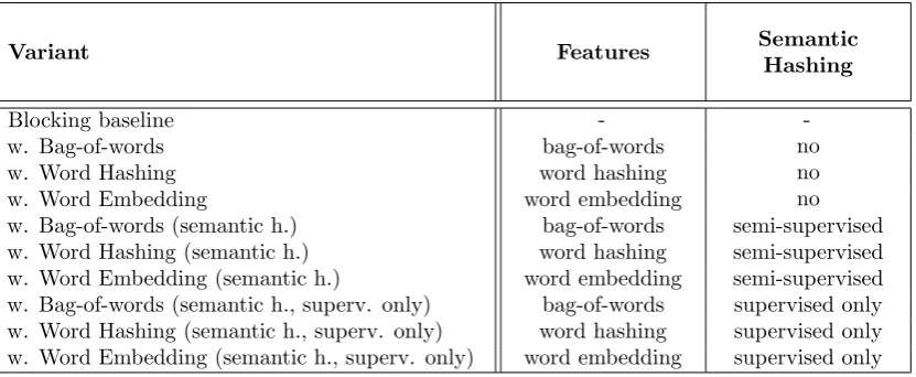
Table 4.3: Overview of the deep learning based indexing algorithm variants.

The table indicates for each variant which additional features (in addition to the base features) are included, how the additional features are encoded.

The implementations for the different word encoding techniques are identical to the implementa-tions used in the matching phase.

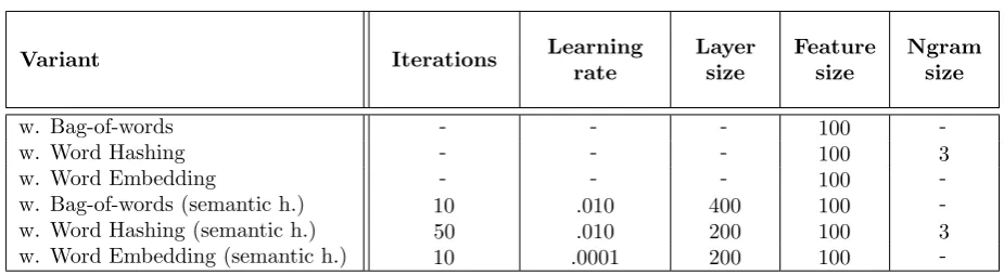
As with the matching variants, the indexing variants have been optimized using the tuning set. In Table 4.4 an overview is given of the hyperparameters for the different variants. In each of the variants the hyperparameters of the genetic algorithm are identical to those in the blocking baseline.

Semantic hashing

In semantic hashing, within an information retrieval context, a document is converted a code by running it through an auto-encoder network. The activation values in the compressed middle layer are then used as the code for the document. In the original application semantic hashing is trained completely unsupervised.

(35)

4.3. INDEXING VARIATIONS 27

Variant Iterations Learning

rate

Layer size

Feature size

Ngram size

w. Bag-of-words - - - 100

-w. Word Hashing - - - 100 3

w. Word Embedding - - - 100

-w. Bag-of-words (semantic h.) 10 .010 400 100

-w. Word Hashing (semantic h.) 50 .010 200 100 3

w. Word Embedding (semantic h.) 10 .0001 200 100

-Table 4.4: Overview of the hyperparameter configuration for each of the indexing variants. The supervised only variants use the same hyperparameter configuration as the corresponding semi-supervised variant. Layer size indicates the size of the bottleneck layer in the auto-encoder network. Feature size indicates the number of additional inputs in the network per token in the record.

concise. In addition, the requirements for automated duplicate detection are generally stricter than for search.

Another difference in usage is that sematic hashing is used in combination with the genetic algorithm. The genetic algorithm and its hyperparameters are identical to the baseline variant. The genetic algorithm is also provided with the original values that are being used in the baseline genetic algorithm variant.

The semantic hashing code is originally a vector of real values. In the original application of document retrieval these values are converted to binary values using a threshold. The threshold is selected so that both bit values are equally likely. The same conversion is applied here, resulting in a number of bit values.

These bit values are used as input for the genetic algorithm. Each of these bit values are provided separately, allowing the genetic algorithm to pick only some of the bit values to use for blocking. This gives the genetic algorithm control more control over the strictness than providing the semantic hashing code as one large value. In addition to the fields containing specific bits from the semantic hashing, the genetic algorithm is also provided with the fields already used in the blocking baseline.

The semantic hashing itself is trained on the input words, represented either using the bag-of-words encoding, word hashing or word embedding. Depending on the variant, training is done either semi-supervised or supervised only. In the semi-supervised variant, the auto-encoder is first trained using unlabeled data. In the supervised step penalties are introduced in the auto-encoder that forces duplicate pairs to have more similar semantic hashes, and non-duplicate pairs to have different semantic hashes.

[image:35.595.48.511.97.224.2]

(36)

4.4 Datasets

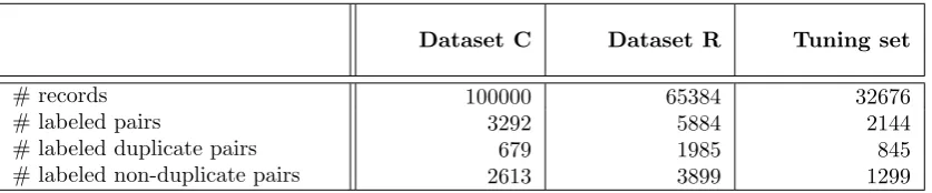
The different algorithms will be evaluated on two datasets in order to compare the differences in performance. In addition, a third dataset, the tuning set, will be used for tuning. All three datasets are samples taken from real-life datasets. As one of the evaluation datasets originates from the same source as the tuning set, there a possibility its results are overly optimistic results. By including a second dataset, finding can be confirmed on a dataset that is not related to the tuning set.

Dataset C Dataset R Tuning set

# records 100000 65384 32676

# labeled pairs 3292 5884 2144

# labeled duplicate pairs 679 1985 845

[image:36.595.108.527.212.299.2]

# labeled non-duplicate pairs 2613 3899 1299

Table 4.5: Overview of the datasets used.

Notice that the tuning set is only used for tuning, not during the actual evaluation.

The datasets have undergone an annotation phase in which a domain expert manually marked pairs as either duplicate or non-duplicate. Although the process of annotating data has been extensive, due to the large amount of possible pairs, only a part of all possible pairs has been annotated. For both datasets the number of records and number of annotated pairs are listed in Table 4.5.

In preparation for the evaluation, all datasets have been preprocessed to make it more suitable for duplicate detection. The preprocessing consists of conversation to lowercase, removal of diacritics and trimming of whitespaces. The preprocessing has been applied indiscriminately to all fields of all records.

The tuning set and dataset R are created using the same original source. To split the original dataset in the two sets the original dataset was split into three parts: two parts were used for dataset R and the third is used for the tuning set. The logic to separate the datasets is the same logic as used during the creation of the K-folds, as described earlier. This method of splitting increases the amount of labeled pairs that is still valid after the splitting, while still assuring that both datasets have no common records (and therefore no common key pairs).

(37)

5

Evaluation results

This chapter contains the results of the evaluation described in Chapter 4. These results will be interpreted and discussed in Chapter 6.

The algorithms listed in the different tables are referred to by a name indicating the algorithm used and a number indicating the training size used. Notice that a training size of ndescribes a classifier trained onn reference pairs marked as duplicate and n reference pairs marked as non-duplicate, resulting in a total reference size of 2n. In addition to marked reference pairs, some algorithms also use unlabeled data.

The main part of the evaluation consists of a K-fold evaluation for both indexing and matching. The results for the indexing algorithms on dataset C are listed in Table 5.4 and in Table 5.3 for dataset R. The results for the matching algorithms are listed in Table 5.2 for dataset C and in Table 5.1 for dataset R.

The complete overview of which of these results are significant can be found in Appendix A. The different algorithms were also evaluated in a training set evaluation: these results can be found in Appendix B.

Reducing labeled data usage in duplicate detection using deep belief networks