Set mapping in the method of imprecision

(1)

Thesis by Xiaoou Wang

In Partial Fulfillment of the Requirements for the Degree of

Doctor of Philosophy

California Institute of Technology Pasadena, California

2003

(2)

c

2003

(3)

Acknowledgements

First I would like to thank my advisor, Professor Erik Antonsson, for his advice and encouragement during the last five years. Almost all my ideas were inspired by the discussions with him. I can not finish this work without his help.

And I also would like to say thanks to some other students at Caltech. I really appreciate the help offered by William S. Law and Michael J. Scott when they already left Caltech. The hardware testing and the solid model were works done by two undergraduates, Zhee Khoo and Juan Nu˜no.

(4)

Set Mapping in the Method of Imprecision

by Xiaoou Wang

In Partial Fulfillment of the Requirements for the Degree of

Doctor of Philosophy

Abstract

The Method of Imprecision, or MoI , is a semi-automated set-based approach which uses mathemat-ics of fuzzy sets to aid the designer making decisions with imprecise information in the preliminary design stage.

The Method of Imprecision uses preference to represent the imprecision in engineering design. The preferences are specified both in the design variable space (DVS) and the performance variable space (PVS). To reach the overall preference which is needed to evaluate designs, the mapping be-tween the DVS and the PVS should be explored. Many engineering design tools can only produce precise results with precise specifications, and usually the cost is high. In the preliminary stage, the specifications are imprecise and resources are limited. Hence, it is not cost-effective nor necessary to use these engineering design tools directly to study the mapping between the DVS and the PVS. An interpolation model is introduced to the MoI to construct metamodels for the actual mapping function between the DVS and the PVS. Due to the nature of engineering design, multistage meta-models are needed. Experimental design is used to choose design points for the first metamodel. In order to find an efficient way to choose design points when a priori information is available, many sampling criteria are discussed and tested on two specific examples. The difference between differ-ent sampling criteria when the number of added design points is small, while more design points do improve the accuracy of the metamodel substantially.

(5)

computeα-cuts with more accuracy and less limitations. The designers have more control over the trade-off between the cost and accuracy of the computation with the new extension of the LIA.

The results of the Method of Imprecision should be the set of alternative designs in the DVS at a certain preference level, and the set of achievable performances in the PVS. The information about preferences in the DVS and the PVS is needed to transfer back and forth. Usually the mapping from the PVS to the DVS is unavailable, while it is needed to induce preference in the DVS from the PVS. A new method is constructed to compute theα-cuts in both spaces from preferences specified in the DVS and the PVS.

(6)

List of Figures

1.1 The rectangle in the plane ofx₉ andx₁₀. . . 3

1.2 The mapping of the rectangle in the plane ofKBandKT. . . 4

3.1 Two approximations of one set of sample data. . . 17

3.2 Geometric model of body-in-white in SDRC I-DEAS. . . 25

3.3 Finite element model of body-in-white. . . 26

3.4 Bending stiffness data projected onto 2 dimensions. . . 28

3.5 (ERMSE/response range) of polynomial and MARS models with 19 design points. 29 3.6 (ERMSE/response range) of polynomial and MARS models with 243 design points. 29 3.7 (ERMSE/response range) of polynomial and MARS models with 3125 design points. 31 3.8 (ERMSE/response range) at all design points. . . 32

3.9 (ERMSE/response range) at all test points. . . 33

3.10 (maximum error/response range) of all design points and test points. . . 34

3.11 (error/response range) at maximum response. . . 36

3.12 Histogram with fitted normal density ofe₁ at10,000random test points. . . 43

3.13 Histogram with fitted normal density ofe₂ at10,000random test points. . . 44

3.14 Ratio of ERMSE to response range of the 10-D function. . . 47

3.15 Ratio of maximum error to response range of the 10-D function. . . 48

3.16 Histogram with fitted Normal density for the errors ofYˆ₁of the 10-D function. . . 49

3.17 Normal probability plot for the errors ofYˆ₁of the 10-D function. . . 50

3.18 Histogram with fitted Normal density for the errors ofYˆ₂of the 10-D function. . . 51

3.19 Normal probability plot for the errors ofYˆ₂of the 10-D function. . . 52

3.20 Histogram with fitted Normal density for the errors ofYˆ₃of the 10-D function. . . 53

3.21 Normal probability plot for the errors ofYˆ₃of the 10-D function. . . 54

(9)

3.23 Ratio of maximum error to response range of the VW model. . . 58

3.24 Histogram with fitted Normal density for the errors ofYˆ₁of the VW model. . . 59

3.25 Normal probability plot for the errors ofYˆ₁of the VW model. . . 60

3.26 Histogram with fitted Normal density for the errors ofYˆ₂of the VW model. . . 61

3.27 Normal probability plot for the errors ofYˆ₂of the VW model. . . 62

3.28 Histogram with fitted Normal density for the errors ofYˆ₃of the VW model. . . 63

3.29 Normal probability plot for the errors ofYˆ₃of the VW model. . . 64

4.1 The preference function of the design variabled₁ord₂. . . 71

4.2 Example result of LIA. . . 72

4.3 The performance functionp=f(d). . . 74

4.4 µd(p)forµdas in Figure 4.1, wherep= 3d3+ 2.5d. . . 75

4.5 The combined design preferences of two design variables by differentPs. . . 77

4.6 P_αd_k’s in a 2-D PVS from a 2-D DVS. . . 78

4.7 P_εd]andP_εd\in a 2-D PVS from a 2-D DVS. . . 81

4.8 Dd₀_.₅(10)’s by different aggregation functions. . . 85

4.9 Pd2 ε (S,U)with different values ofT andU. . . 86

4.10 µd1(d1),µd2(d2),µp₁(p1)andµp₂(p2). . . 90

4.11 The shape ofµo(d~). . . 91

4.12 Do2 0.5(S)for different values ofS. . . 92

4.13 Po2 0.5(S,U)for different values ofS andU. . . 93

4.14 Pd2 0.5(8,16)andPo 2 0.5(8,16)by the forward calculation. . . 94

4.15 Po2 0.5(8,16)by the new method andPo 2 0.5(1,1)andPo 2 0.5(8,16)by the forward calcu-lation. . . 95

5.1 Testing setup of body-in-white. . . 101

5.2 Geometric model of body-in-white in SDRC I-DEAS. . . 102

5.3 Finite element model of body-in-white. . . 102

5.4 Design preferences of the VW model. . . 104

5.5 Functional requirements of the VW model. . . 105

5.6 Aggregation hierarchy of preferences. . . 106

5.7 Theα-cuts of design variables atd~∗. . . 109

(10)

5.9 Theα-cuts of performance variables atp~∗. . . 113 5.10 The cross sections ofPαo2

k at~p

(11)

List of Tables

3.1 Data Fitting Models. . . 27

3.2 Selected Numerical Results. . . 30

3.3 Error at Maximum Response (3,364.9). . . 35

3.4 Ratio of ERMSE to Response Range of the 10-D Function. . . 46

3.5 Ratio of Maximum Error to Response Range of the 10-D Function. . . 47

3.6 Significance Levels of Different Tests on the 10-D Function. . . 50

3.7 Ratio of ERMSE to Response Range of the VW Model. . . 56

3.8 Ratio of Maximum Error to Response Range of the VW Model. . . 56

3.9 Significance Levels of Different Tests on the VW Model. . . 60

(12)

Chapter 1 Introduction

The Method of Imprecision, or MoI , is a semi-automated set-based approach which uses the mathe-matics of fuzzy sets to aid the designer making decisions with imprecise information in the prelim-inary design stage [62, 28].

In the preliminary design stage, imprecision is the design engineer’s uncertainty in choosing among alternatives, and it arises primarily from choices not yet made because of the intrinsic vague-ness in the design description, and the uncertainty in the specifications and requirements. Precise information is usually impossible to obtain. As the design proceeds from the preliminary stage to de-tailed design and analysis, the level of imprecision is reduced. Finally, the design description will be precise, except for tolerances, which represent the allowable uncontrolled manufacturing variation. Despite the unavoidable imprecision in the preliminary design stage, engineering design methods and computer aids require precise information. The MoI was developed to represent and manipu-late the imprecise information in the preliminary design stage because the designer faces the highest imprecision, and the most expensive decisions are made, in the preliminary stage [21, 56, 60, 57].

An imprecise variable in the preliminary design may potentially take on any value within a possible range. Although the nominal value of the imprecise variable is unknown, some values are preferred more than others by the designer. The method of imprecision borrows the notion of membership functions in a fuzzy set to represent the preference among designs. Although the preference function in the MoI and the membership function in the fuzzy sets both have values from 0to1.0, they are different. The membership function models the uncertainty in categorization. The preference function is fuzzy in unresolved alternatives.

(13)

“optimal” design. But the information is only available near that single point. In contrast, the MoI is a set-based method. Sets of designs are evaluated in the MoI. The case study of Toyota’s design and development process shows that set-based methods enable effective communication, allow greater parallelism, and permit early decisions based on information that is not yet precise [59, 58, 32, 55]. In the MoI , the design engineers identify preferences on each of the performance variables by which each design alternative will be evaluated. These preferences will typically come from poten-tial customers. The designers also identify preferences on design variables (dimensions, material properties, etc.). These preferences will come from the designers’ experience and judgment, and are subject to change as the design process proceeds. One of the central aspects of the MoI is map-ping the preferences from design variables onto the performance variables, and then building an aggregate overall preference.

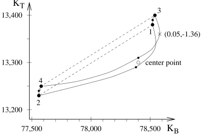
Many people have contributed to the MoI , and one design tool (IDT) was built by William S. Law [27, 28]. In his Ph.D. thesis, William asked several questions about the implementation of the MoI based on an example in [26]. This example is the mapping of a rectangle in the plane of two design variables x₉ and x₁₀ to the plane of two performance variables bending stiffness KB and torsional stiffnessKT. The approximation ofKB is shown in Equation 1.1, and the approximation ofKT is shown in Equation 1.2.

KB = 78,400 + 170x9−240x10−630x92−5x9x10−88x102 (1.1)

KT = 13,300 + 130x9−38x10−620x92+ 5x9x10+ 4x102 (1.2)

The plane ofx₉andx₁₀is shown in Figure 1.1. The center points, the four corner points, four center points on the boundaries, and the boundary are mapped to the plane of KB and KT. The results of the mapping are shown in Figure 1.2. The solid lines are the mapping of the boundary in Figure 1.1. The dashed lines connect the mapping of four corner points. The maximum of

(14)

x

₉

x

₁₀

2

3

4

(0,2)

(-0.05,0)

(0,-2)

(0.05,0)

1

(0.05,-1.36)

center point

Figure 1.1: The rectangle in the plane ofx₉andx₁₀.

by optimizations. Each approximation listed above has its advantages and disadvantages. Several questions generated from this example need to be answered:

1. Is the linear approximation sufficiently accurate for preliminary engineering design?

2. Will a nonlinear approximation of the mapping functions increase the accuracy of the bound-ary, but not increase the computation cost significantly?

3. Which approximations are the most accurate and the most flexible among the three approxi-mations discussed above, or is there any other method to approximate the boundary?

4. Is there any way to let the designer make a compromise or trade-off between the cost and the accuracy with which the boundary is approximated?

1.1 Organization of Thesis

(15)

K

_B

78,000

3 78,500

77,500

13,200

13,300

13,400

1 K

_T

center point

2

4 (0.05,-1.36)

Figure 1.2: The mapping of the rectangle in the plane ofKBandKT.

Their work has laid a broad theoretical foundation and practical implementation for the method of imprecision.

The work described in this thesis seeks to improve the accuracy and efficiency of the imple-mentation of the MoI , by practical testing via specific examples. Its principal contributions are the introduction of a multistage nonlinear metamodel into the MoI , a new extension of the LIA, and a new method to compute the overall preference with loose constraints.

Chapter 2 introduces basic concepts and techniques in the MoI . Section 2.1 defines the basic concepts such as variables, spaces and preferences. The overall preference, which is used to evaluate the design, is introduced in Section 2.2. Aggregation functions and rational aggregation are also discussed in the same section. Section 2.4 presents the family of rational aggregation functions.

(16)

in Sections 3.8 and 3.9.

Chapter 4 presents the efficient and accurate computation of the overall preferences. The ex-tension principle and the LIA are introduced in Section 4.1. Then some anomalies and limitations of the original LIA implementation are discussed in Section 4.2. Section 4.3 introduces some ex-tensions of the original LIA. The methods to compute overall preferences in both DVS and PVS withoutf~−1are discussed in Section 4.4.

Chapter 5 presents the full new implementation of the MoI . The models and methods discussed in Chapters 3 and 4 are combined into the new implementation of the MoI in Section 5.1. A measure of the sensitivity of the α-cuts to the metamodel is also proposed in Section 5.1. In Sections 5.2 to 5.4, the new implementation of the MoI is demonstrated on a practical design problem, and the results are compared with previous results.

(17)

Chapter 2 The Basics of the Method of Imprecision

This chapter will focus on the basic concepts and techniques in the Method of Imprecision [62, 28]. Section 2.1 defines the basic concepts such as variables, spaces and preferences. The overall preference which is used to evaluate each design is introduced in Section 2.2. Aggregation functions and axioms for rational aggregation are also discussed in the same section. Section 2.4 presents a family of the rational aggregation functions.

2.1 The Basic Concepts

The design variables, {d₁, . . . , dn}, are independent variables which differentiate alternative de-signs. There may be other attributes of the design which are not included in the design variables because they are not required to identify different designs. The design variables can be discrete or continuous, but they are at least ordinal in order to facilitate computations. The independence between design variables does not imply that design variables can not be related, but means that the value of each design variable can be freely chosen.

All alternative designs under consideration form the design variable space or DVS. The set of valid values for the design variablediis denotedXi. All design variables form ann-vector,d~, which distinguishes one particular alternative design from others in the DVS.

DV S=x₁×x₂× · · · ×xn [ Cartesian Set Product ] (2.1)

(18)

performance variables for each alternative design form aq-vector, ~p = f~(d~), which specifies the quantified performances of a designd~. The performance variable space, or PVS, is the set of all quantified performances achievable by all designs in DVS, wheref~(d~) ={f₁(d~), . . . , fq(d~)}. The mapping function fj(d~) can be any calculation, such as closed-form functions, empirical “black-box” functions, physical experiments, or even from consumer surveys.

P V S ={~p|~p=f~(d~), ∀d~∈DV S } ⊆p₁×p₂× · · · ×pq (2.2)

The design variables and performance variables are imprecise in nature. The final value of each variable is unspecified, and only the range of each variable is known in the preliminary stage of the design. But certain values in the range are preferred more than others. The preference can be used to quantify the imprecision of each variable.

The functional requirementµpj(pj)represents the customer’s direct preference for values of the performance variablepj, which may be specified by customers, or estimated by the designers:

µpj(pj) :Yj →[0,1] (2.3)

The functional requirements preferences are based on quantified aspects of design performances represented by performance variables. Other unquantified aspects of design performance such as style are usually not modeled by performance variables; the preferences of these aspects are repre-sented by the design preferences. The design preference functionµdi(di)represents the designer’s preference for values of the design variable di, which will be specified by the designers based on design considerations:

µdi(di) :Xi →[0,1] (2.4)

2.2 The Aggregation Functions

(19)

is called the overall preference, which can be expressed in the DVS asµo(d~):

µo(d~) =P

µd₁(d1), . . . , µdn(dn), µp1(f1(d~)), . . . , µpq(fq(d~))

(2.5)

The overall preference of the achievable performance can also be expressed in the PVS asµo(~p):

µo(d~) =P µd₁(~p), . . . , µdn(~p), µp1(p1), . . . , µpq(pq)

(2.6)

TheP in Equation 2.5 is the aggregation function, which reflects how the competing attributes of the design should be traded off against each other [40, 41], and formalizes the designer’s balanc-ing of conflictbalanc-ing goals and constraints. In order to model the designer’s trade-off strategy, some restrictions must be applied on the aggregation functions to maintain their rationality [38]. These restrictions are described by the following five axioms, whereN =n+q.

Axiom 2.1 Commutativity:

P(µ₁, . . . , µj, . . . , µk, . . . , µN) =P(µ1, . . . , µk, . . . , µj, . . . , µN) ∀1≤j, k ≤N

This axiom indicates the aggregation function’s independence on the order in which the indi-vidual preferences are combined.

Axiom 2.2 Monotonicity:

P(µ₁, . . . , µk, . . . , µN)≤ P(µ1, . . . , µ0k, . . . , µN) forµk ≤µ0_k, ∀1≤k≤N .

The monotonicity means that the change of the overall preference caused by any change in any individual preference should not move in the opposite direction. If the monotonicity is not satisfied, an increase in one individual preference will cause decrease in the overall preference, which is not rational.

Axiom 2.3 Continuity:

P(µ₁, . . . , µk, . . . , µN) = lim µ0_k→µk

P(µ₁, . . . , µ0_k, . . . , µN) ∀k

(20)

Axiom 2.4 Idempotency:

P(µ, . . . , µ) =µ

The idempotency will remove the artificial biasness in the aggregation function.

Axiom 2.5 Annihilation:

P(µ₁, . . . ,0, . . . , µN) = 0

A preference of zero indicates that the value of that variable is totally unacceptable. This axiom is needed to make sure that any acceptable design does not have any unacceptable design perfor-mance.

These five axioms are only necessary conditions for the rationality of the aggregation function. Similar axioms are defined by Fung and Fu [20] to maintain the rationality in general decisionmak-ing: commutativity, monotonicity, continuity, idempotency, and associativity. It is noted that the annihilation axiom is not necessary for the rationality of general decision-making.

The aggregation functions satisfying all above axioms are considered design-appropriate. Al-though there are many design-appropriate aggregation functions, the choice should be made accord-ing to the relationship between design and performance variables as follows [42, 64].

In one type of design strategy, the overall preference of the system is determined by the lowest preference on any variable. The increase in preference for one variable can not compensate for the decrease in another preference. There is no trade-off between individual preferences. This is a non-compensating trade-off strategy. The minimum aggregation function Pmin should be used here:

µo= min (µd1, . . . , µdn, µp1, . . . , µpq) (2.7)

Pmin is the hard “and” operation in fuzzy logic [4], which will lead to the classic max-min solution from game theory [65].

In another type of design strategy, the decrease in one preference can be counterbalanced by the increase in another, that is, the two preferences can be traded off with each other. This is a fully compensating trade-off strategy. The geometric weighted mean functionP_Πis needed:

µo=

 Yn

i=1

µdi· q

Y

j=1

µpj

 

1 n+q

(21)

PΠis the soft “and” operation in the fuzzy logic [4], which corresponds to the Nash solution

from game theory [65].

2.3 Weights of Preferences

The variables representing a design are not equally important with each other. The relative impor-tance of each variable can be specified by assigning weights to the corresponding variables:

ωdi ≥0

ωpj ≥0

Now the overall preference should be aggregated from both the individual preferences and the individual weights. The axioms which the aggregation functions should satisfy need to be redefined in order to include weights:

Axiom 2.6 Commutativity:

P(µ₁, . . . , µj, . . . , µk, . . . , µN; ω1, . . . , ωj, . . . , ωk, . . . , ωN) =

P(µ₁, . . . , µk, . . . , µj, . . . , µN; ω1, . . . , ωk, . . . , ωj, . . . , ωN) ∀j, k

Axiom 2.7 Monotonicity:

P(µ₁, . . . , µk, . . . , µN; ω1, . . . , ωk, . . . , ωN)≤ P(µ1, . . . , µ0k, . . . , µN; ω1, . . . , ωk, . . . , ωN) for µk< µ0k, ∀k

P(µ₁, . . . , µk, . . . , µN; ω1, . . . , ωk, . . . , ωN)≤ P(µ1, . . . , µk, . . . , µN; ω1, . . . , ω0k, . . . , ωN) for ωk< ωk0, where µj ≤µk, ∀j6=k, ∀k

The overall preference should not decrease if the weight of the variable with the highest prefer-ence is increased.

Axiom 2.8 Continuity:

P(µ₁, . . . , µk, . . . , µN; ω1, . . . , ωk, . . . , ωN) = lim

µ0_k→µk

(22)

lim ω0_k→ωk

P(µ₁, . . . , µk, . . . , µN; ω1, . . . , ω0k, . . . , ωN) ∀k

The aggregation function should have continuities on both preferences and weights.

Axiom 2.9 Idempotency:

P(µ, . . . , µ; ω₁, . . . , ωN) =µ

Axiom 2.10 Annihilation:

P(µ₁, . . . ,0, . . . , µN; ω1, . . . , ωk, . . . , ωN) = 0 whereωk 6= 0, ∀k P(µ₁, . . . , µk, . . . , µN; ω1, . . . ,0, . . . , ωN) =

P(µ₁, . . . , µk−1, µk+1, . . . , µN; ω1, . . . , ωk−1, ωk+1, . . . , ωN) ∀k

If a variable is assigned a weight of zero, that variable will be removed from the aggregation. Because no upper boundaries and normalizations are specified on the weights in the definition, an additional axiom is needed:

Axiom 2.11 Self-normalization:

P(µ₁, . . . , µN; λ ω1, . . . , λ ωN) =P(µ1, . . . , µN; ω1, . . . , ωN) where λ >0

According to the self-normalization axiom, the weights can be scaled by any positive constantλ

without any change in the overall preference. A weighted aggregation function is design appropriate if all above six axioms are satisfied.

2.4 Weighted Means

The theory of functional equations [1] has been applied to the exploration of certain aggrega-tion funcaggrega-tions called t-norms and t-conorms [14]. The same approach was applied to the design-appropriate aggregation functions by Scott and Antonsson [50]. The relevant class of functions is the weighted means:

P(µ₁, . . . , µN; ω1, . . . , ωN) =g

PN

i=1ωig−1(µi)

P_N

i=1ωi

!

(23)

wheregis a strictly monotonic, continuous function with inverseg−1;g(0)≤µi ≤g(1),ωi ≥ 0, 1 ≤ i≤ N; andPN_i₌₁ωi >0. It is shown that the weighted means satisfy all the axioms except possibly the annihilation axiom. Then all weighted means which satisfy the annihilation axiom are design-appropriate. Arbitrary design-appropriate aggregation functions also satisfy other prop-erties with the assumption of strict monotonicity [50]. Any strictly monotonic design-appropriate aggregation must be a weighted mean.

The family of weighted root-mean-power functions is generated by the functiong(µ) =µs[1]:

Ps(µ1, . . . , µN; ω1, . . . , ωN) =

PN i=1ωiµsi

P_N

i=1ωi

!1 s

(2.10)

where s ∈ R. If s > 0, 0 =g(0)≤µi≤g(1) = 1. If s < 0, g−1(µ) and Ps satisfies the annihilation axiom [50]. Ps≤0 is a family of design-appropriate aggregation functions because it satisfies all the axioms in Section 2.3.

The two design-appropriate aggregation functions,PminandPΠ, are just limiting cases ofPs≤0 wheres→0 &s→ −∞respectively [50]:

PΠ=Ps=0(µ1, . . . , µN; ω1, . . . , ωN) = N

Y

i=1

µωi di

!1 ω

where ω=PN_i₌₁ωi (2.11)

and

Ps=−∞(µ1, . . . , µN; ω1, . . . , ωN) = min(µ1, . . . , µN) (2.12)

OtherPswith−∞< s≤0changes continuously withsbetweenPminandPΠand represent partially compensating trade-off strategies, where a change of preference for one variable can be

partially compensated for by changing the preference for another variable.

Because of the properties of idempotency and monotonicity,Pminis the lower bound for design-appropriate functions. Similarly,Pmax = max(µ1, . . . , µN)might be the upper bound for design-appropriate functions. ButPmaxis not design-appropriate because it does not satisfy the annihila-tion axiom.

(24)

because of the actual implementation of the MoI [48].

The parametersdefines the trade-off strategy or degree of compensation between any two vari-ables, and is implemented by a design-appropriate aggregation functionPs(µ1, µ2; ω1, ω2). The indifference points are defined as two points which have the same preference. The parametersand the weights can be numerically calculated from indifference points [52].

2.5 Hierarchical Aggregation

If many different trade-off strategies are used to aggregate the overall preference in a design, the in-dividual preferences should be aggregated by an aggregation hierarchy. The hierarchy is determined by the problem. Even if differentPs’s are used in the hierarchy, the weights can be propagated freely because of the self-normalization axiom discussed in Section 2.3. If there are only aggregations of pairs of individual preferences in the hierarchy, a numerical method can be used to calculate the parametersand the weights [52].

One special situation for hierarchical aggregation is aggregations with the samesthat are com-bined together. Consider three individual preferences µ₁,µ₂ and µ₂ with weightsω₁, ω₂ and ω₂. Assumeµ₁is first aggregated withµ₂, then aggregated withµ₃with the same trade-off strategy.

Ps(Ps(µ1, µ2; ω1, ω2), µ3; ω1+ω2, ω3) (2.13)

=

(ω₁+ω₂)Ps(µ1, µ2; ω1, ω2)s+ω3µs₃ (ω₁+ω₂) +ω₃

1 s =     

(ω₁+ω₂)

(ω₁µs 1+ω2µs

2) 1 s ω1+ω2

s

+ω₃µs₃ ω₁+ω₂+ω₃

     1 s =

ω₁µs₁+ω₂µs₂+ω₃µs₃ ω₁+ω₂+ω₃

1 s

= Ps(µ1, µ2, µ3; ω1, ω2, ω3)

(25)

2.6 Summary

All designs under consideration form the DVS, and the design variables, are used to distinguish alternative designs. The PVS consists of all achievable performances. The performance variables can be mapped from the vector of design variables. All quantified preferences are specified on the performance variables directly, usually in consultation, or by survey, of the customers. Other unquantified preferences are determined by the designer based on judgment and experience.

The design will be evaluated by the overall preference which is aggregated from individual preferences. A design with higher overall preference is preferred more than one with lower over-all preference. The aggregation functions embody the trade-off strategies. All design-appropriate aggregation functions represent rational trade-off strategies and satisfy the five axioms: commu-tativity, monotonicity, continuity, annihilation, and idempotency, among which the annihilation is unique to design problems.

Weights may be included in the aggregation function in order to represent the relative impor-tance of individual preferences. In this case, all of the above five axioms need to be redefined, and one self-normalization axiom is added for the scalability of weights.

The family of root-mean-power functions Ps with a negative parameters, P−∞<s≤0, contain all monotonic design-appropriate aggregation functions. The root-mean-power function Ps with positive parameters >0is not design appropriate, but it can be modified to be design appropriate because of the implementation details of the MoI, as shown later. If different trade-off strategies are used in a design, a hierarchy of aggregation is needed.

(26)

Chapter 3 Metamodels for the Mapping between DVS and PVS

A central element of the MoI, is to approximate the mapping between the design variable space (DVS) and the performance variable space (PVS), because the mapping will be used to induce preferences in the PVS from the preferences in the DVS, as will be discussed in Chapter 4. Because of the wide use of computers, this process is usually conducted by running some complex computer analysis software package. When the DVS is high dimensional, it is prohibitively expensive to directly use complex analysis software to explore the DVS. For example, it will require about 5 minutes to analyze a modestly complex finite element model. For a five dimensional DVS, it will require about 10 days on a grid with 5 points on each design variable (DV). If the dimensionality of the DVS increases to 10, then it will run about 92 years, on a grid with 5 points on each DV.

It is not necessary to pursue high accuracy at the preliminary stage of the engineering design. So, a linear approximation can often be used to reduce the computational cost [30]. It does not perform well on nonlinear mappings common in design, so a traditional optimization is used to improve the accuracy [30]. It is preferred to have one single model to estimate linear and nonlinear mappings.

A metamodel is defined as “a model of the model [24].” It should have flexible model structure and be able to estimate the actual mapping with reasonable accuracy. A metamodel will be con-structed by running the analysis software over a relatively small set of design points, and will be used to explore the mapping between the DVS and the PVS. Due to the iterative nature of engineer-ing design, multistage metamodels are helpful, because a more accurate metamodel may be needed as the design is refined.

(27)

at the first stage. In Sections 3.4 and 3.5, the base functions used in the metamodel will be deter-mined by tests on two specific examples. The sampling criteria of the design points, when there is a priori knowledge available, will be discussed in Section 3.6. Section 3.7 introduces two methods

to test the improvements between metamodel at different stages. Finally, the sampling criteria will be tested on two specific examples in Sections 3.8 and 3.9.

3.1 Approximation or Interpolation

The difference between a computer experiment and a traditional physical experiment is that repeated computer experiments generate the same results.

For an approximate model of a traditional physical experiment, the most frequently used method is least-squares regression, which models the random errors in the results as identical and indepen-dent Normal variables with mean zero and varianceσ, that is,εrandom ∼N(0, σ2). The least-square estimator will minimize the sum of the squared differences between the experiment results and the predicted values. Figure 3.1 shows one set of sample data and the results of two different approxi-mate models. The relationship between the estiapproxi-mate and the actual value is

y= ˆy+εsystem+εrandom (3.1)

whereyis the actual value,yˆis the estimated value,εsystemis the systematic error, andεrandomis the random error, or call it approximation error.

Although the estimated model does not pass through the actual values, it is assumed that the random errors are smoothed out because of the assumption ofεrandom ∼N(0, σ2)

However, for the deterministic results from a computer experiment, the relationship between the estimate and the actual value is

y= ˆy+εsystem (3.2)

whereyis the actual value,yˆis the estimated value, andεsystemis the systematic error.

Although the response surface method is based on least square regression, it still can be applied to computer experiments if the dimensionality of the design space is not high and the response is not strongly nonlinear, because of the simplicity and maturity of the response surface method.

(28)

Sample Data

Cubic Approximation Linear Approximation

(29)

high-dimensional computer experiments. But the fatal disadvantage of the neural networks is that it converges slowly. To construct a good metamodel, it needs lots of training data. This makes the neural networks not suitable for building the metamodel in the preliminary stage of engineering design where available resources are limited.

Inductive learning draws inductive inference from obtained facts [17, 16]. This method builds the estimation model in the form of condition-action rules, and decision trees. A matched rule is found by a search in the decision tree for the encountered condition [25]. This method works well if the design variables and the response are almost all discrete-valued, but it is not a good candidate in engineering design where, in general, the responses are continuous

By probabilistic modeling of the uncertain prediction error, J. Sacks et al. proposed a new in-terpolation model which generates the best unbiased linear predictor for the deterministic computer experiment [46]. This method is discussed in detail in the next section.

3.2 Interpolation Model

Consider the approximation ofY(x)by someYˆ(x)wherex ∈ Rm. In Equation 3.2, the structure of the systematic error system is usually unknown. In the approach proposed by Sacks, Schiller and Welch [46], the estimate is an approximation, Pk_j₌₁βj ·fj(x), and system is modeled as a stochastic process,Z(x). Now the model becomes

Y(x) = k

X

j=1

βj·fj(x) +Z(x) (3.3)

The approximation is simple and straightforward once the choice of the base functions fj is made. For the stochastic process Z(x), the important part is the covariance structure, and this is chosen to be

Cov(Z(t), Z(u)) = V(t, u)

= σ_z2·exp(−θ·

m

X

j=1

(tj−uj)pj) (3.4)

wheret= (t₁, . . . , tm)and u = (u1, . . . , um),σ2z,pj andθ >0 are parameters to be decided by the designer.

(30)

affect the prediction ability of the model. It is harder to predict for the model with larger θthan the model with smallerθ. The choices ofpj’s will determine the derivatives of the correlation functions and the response. Here thepj’s are chosen to be2, andθis set to1/2.

The points in the DVS used to build the estimation model are called the design points. With a set of n design points, S = {s₁, . . . , sn} and corresponding response Y(s1), . . . , Y(sn), the interpolation model is generated as follows by Sacks, Schiller and Welch [46]. First introduce the notation:

β = [β₁, . . . , βk]

V = [Cov(Y(si), Y(sj)]1≤i≤n,1≤j≤n

f_x0 = [f₁(x), . . . , fk(x)]

v_x0 = [V(s₁, x), . . . , V(sn, x)]

y0 = [Y(s₁), . . . , Y(sn)]

F = [fl(si)]1≤i≤n,1≤l≤k (3.5)

For the linear predictor of the response,c0·y, its mean square error (MSE) is [46]:

E[c0·y−Y(x)]2 = (c0·F ·β−f_x0 ·β)2+ [c0,−1]·

 

 V vx v_x0 σ_z2

  ·

   c

−1

 

 (3.6)

To obtain an unbiased predictor, it is needed to apply the constraintF0·c=fx. After minimizing the MSE for the predictor c0 ·y under the above constraint by Lagrange multipliers method, the interpolation model becomes [46]

ˆ

Y(x) = f_x0 ·βˆ+v_x0 ·V−1·(y−F ·βˆ) ˆ

β = (F0·V−1·F)−1·F0·V−1·y (3.7)

(31)

3.3 Experimental Design

Experimental design methods have been widely used in many areas including computer experi-ments. It helps to learn how systems work. Careful design of experiments will result in improved process yields, reduced development costs, etc. It also has an important role in the area of engi-neering design. It helps the designer to compare different design configurations, to optimize design parameters, to improve robustness of the design, etc. The design of experiment also helps to choose design points which are used to construct the metamodel efficiently.

There are many frequently used experimental design methods for different purposes. One such method is Latin Hypercube sampling first introduced by M.D. Mckay et. al. [35], which ensures all portions of the design space are sampled. The Latin Hypercube method is an extension of stratified sampling. With stratified sampling, the design space is divided into many disjoint strata. Each stra-tum is sampled individually. The Latin Hypercube simply divides the region of each design variable into N strata with equal marginal probability distribution. If the design variables are distributed equally, each stratum will be divided into the same range, and then the method is called Uniform Latin Hypercube sampling. Each stratum is sampled only once. Therefor, for theith design vari-able, there will be N different sampling locations{dvi,1,· · ·, dvi,N}. The values of theithdesign variable at all N sampling points, {xi,1,· · ·, xi,N}, will be a permutation of {dvi,1,· · ·, dvi,N}. Because all portions of each design variable region are covered in the Latin Hypercube sampling, it is best used when there are only a few dominating design variables for the response. The Latin Hypercube method usually needs a reasonably large number of samples to make the method work well.

(32)

fixed values are called the generators. WithP independent generators, the2k−pfractional factorial design can be constructed, which is1/2p fraction of the2kfactorial design [37, Page 398]. There are many possible choices of generators, but only some of them can generate the highest possible resolutions. If two or more effects can not be differentiated by the observations, they are called aliases [37, Page 374]. The resolution of a fractional factorial design is considered to be K ifn -factor effects and effects with less than (K−n)-factor are not aliases [37, Page 376]. The most useful ones are Resolution III designs, Resolution IV designs, and Resolution V designs.

For a Resolution III design, no two or more main effects are aliases, but any main effect and any two-way interactions may be aliases. For a Resolution IV design, no two or more main effects are aliases, neither are any main effects and any two-way interaction. But two or more two-way interactions may be aliases. For a Resolution V design, no two or more main effects are aliases, neither are two or more two-way interactions. But any two-way interaction and any three-way interaction may be aliases [9].

If the regression model is only first-order, the orthogonal first-order designs [37, Page 600] can be used to minimize the variance of the regression parameters. A design is orthogonal if the matrix (X0X) is diagonal. The 2k _{factorial design and fractional factorial design are both orthogonal.} Another type of orthogonal design is the simplex design [11]. The simplex design is a equilateral triangle fork= 2, and is a regular tetrahedron fork= 3.

For fitting the second-order polynomial regression model, the central composite design, or CCD [37, Page 601], is the most popular design. Usually the CCD consists of a Resolution V

fractional factorial design, the center point, and2·kaxial points forkfactors. There are several variations of CCD. If the fractional factorial design in the CCD is only Resolution III, the design is called small composite design [37, Page 605]. Sometimes the interesting region is thek-dimensional hypercube, then the axial points can be put at the center of each face, i.e.,±1. This design is called the face-centered central composite design [37, Page 605].

The Box-Behnken design, proposed by Box and Behnken, is also used for the second-order regression model [5]. It is constructed by combining the 2k factorial design and the incomplete block design. This type of design is spherical design. All the design points are on a sphere of radius

√

2, and there are no corner points included.

(33)

factors.

3.4 Base Functions

For the first part of Equation 3.3, the base functionsfj(x)are unspecified. The second part of the Equation 3.3 models the error in the approximation of the response. The general principles of choos-ing a good model type are flexibility and parsimony, and a trade-off is always made between them. In the preliminary stage of engineering design, the computational cost is a significant concern, so more weight is put on the principle of parsimony when considering the model type of base func-tions. Also, there is the “main effects principle,” which is the empirical observation that linear main factors are more important than high-order interactions [34]. From all of the above considerations, several polynomial models ( from the simple linear model, quadratic model, to more complicated nonlinear MARS model ) are candidates for the base functions in the interpolation model.

3.4.1 Polynomial Models

The linear model ofnindependent variables with up tomorder interactions is

ˆ

ylinear= ˆf(x1, . . . , xn) = a0+ n

X

i=1

aixi (3.8)

The design points for the linear model are determined by a Resolution III fractional factorial design. In piecewise linear model, the design variable space is divided into many rectangular subspaces and each subspace has its own linear model, as above.

The (partially) quadratic model ofnindependent variables with up tomorder interactions adds quadratic terms to the linear model above:

ˆ

yquad= ˆf(x1, . . . , xn) = ˆylinear(x1, . . . , xn) + n

X

i=1

aiix2i (3.9)

The central composite design is used to decide the coefficients of the quadratic terms. It is simply the factorial design plus the central points of each face.

(34)

by the values ofnandm, is

ˆ

y= ˆf(x₁, . . . , xn) = a0+ n

X

i=1

aixi+ n

X

i1=1 n

X

i2=1

ai1i2xi1xi2+, . . . ,

+ n

X

i1=1

. . .

n

X

im=1

ai1...imxi1. . . xim (3.10)

This is equivalent to a product of several linear regression polynomials. If the number of data points is less than the number of terms in the polynomial, only the coefficients of an equal number of lower-order terms are nonzero.

3.4.2 Nonlinear Regression MARS Model

MARS [19, 45] fits high-dimensional data to an expansion in multivariate spline basis functions. The number of basis functions, the product degree, and the knot locations are automatically deter-mined by, and are adaptive to, the data. The model produces a strictly continuous approximation with continuous derivatives, and identifies the contributions from additive terms and multivariable interactions. The method is attractive due to its low computational cost.

“The approximation takes the form of an expansion in multivariate spline basis func-tions:

ˆ

y= ˆf(x₁, . . . , xn) =a0+ M

X

m=1

amBm(x1, . . . , xn) (3.11)

with:

B₀(x₁, . . . , xn) = 1, (3.12)

Bm(x1, . . . , xn) = KYm

k=1

bkm(xv(k,m)|tkm). (3.13)

The{am}M₀ are the coefficients of the expansion. Each multivariate spline basis func-tion Bm is the product of univariate spline basis functions b, each of a single in-put variable x_v₍_k,m₎, and characterized by a knot at tkm. The multivariate spline basis functions Bm are adaptive in that the number of factors Km, the variable set

V(m) ={v(k, m)}Km

1 , and the parameter settkm are all determined by the data.” [18, Page 17]

(35)

Based on modeling of five-dimensional input variables on an engineering workstation, results can be obtained essentially immediately when 32 observations are used and a maximum of 30 base functions are allowed. The regression computations required less than 80 seconds for modeling and prediction based on 3125 data points with a maximum of 40 base functions.

Another advantage of MARS is that it provides methods of slicing up the n-dimensional space by assigning specific values to a subset of the design variables and obtaining the MARS model along the slice. This is of great convenience when the shape of performance response in one or two specific directions is needed.

3.5 Method for Selection of the Base Functions

Among the candidates listed in Section 3.4, one type of base function will be chosen. The choice will be made based on the performance of each type of base functions on a practical problem described below. One estimation model will be built for each type of base function using the least-squares regression method. This finite element model has already been run on a55 grid in the DVS. There are55 = 3125points in the DVS and corresponding values of the response at these points. Only a fraction of the results will be used to build the estimation model, but all data will be used to evaluate the performance of the resulting model. All the points used to test the model are called the test points. For each estimation model, the empirical root-mean-square error (ERMSE) at all the design

points and all the test points, the maximum error at all design points and test points, and the error at the point with maximum response will be computed as the measure of the performance of each type of base function. Also, the cost of building the model will be taken into consideration. Because the computation cost of the least square regression method is negligible when compared with the cost of the finite element model, only the latter cost, i.e., the number of design points, will be considered.

3.5.1 Problem Description

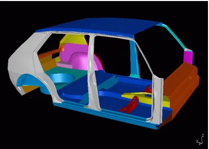
The test function in the example presented here is the bending stiffness of a Volkswagen passenger automobile chassis (shown in Figure 3.2) computed from a finite-element model (shown in Fig-ure 3.3) in a design space of five variables (n= 5):

x₁ = A Pillar Thickness [mm]

(36)

Figure 3.2: Geometric model of body-in-white in SDRC I-DEAS.

x₃ = Floor Rail Thickness [mm]

x₄ = Floor Thickness [mm]

x₅ = B Pillar Location [mm]

Table 3.1 lists the models that have been built to fit the actual response function. In all cases,

n=5. For the linear model (LM),m= 2was used for 17 points which are a Resolution IV fractional factorial design and the center point, andm= 5was used for 32 points which are the full factorial design. For the quadratic model (QDM),m= 2for 14 and 19 points. The 14 points are a Resolution III fractional factorial design, the center point, and five face-center points{d₁, . . . , d₅}where

dk = 1and dl = 0, ∀ l 6= k,1 ≤ k ≤ 5. The 19 points are a Resolution III fractional factorial design, the center point, and ten face-center points{d₁, . . . , d₅}wheredk=±1and

(37)

Figure 3.3: Finite element model of body-in-white.

with 243 points which is the combination of 32 2-level full factorial designs in 32 sub-hypercubes, and 1024 linear models in the PLM with 3125 points which is the combination of 1024 2-level full factorial designs in 1024 sub-hypercubes. The test points for each model are all points on the 55 grid except the design points.

3.5.2 Test Results

Figure 3.4 shows a projection of the five-dimensional bending stiffness data surface onto 2 dimen-sions (Floor thickness and B pillar location). This illustrative projection was created by holding each of the 3 dimensions not shown (A pillar thickness, B pillar thickness and Floor rail thickness) at a constant value. The approximations computed here fit all 5 dimensions of the design space, however, to enable graphical comparison, the figures only show variations in bending stiffness as a function of 2 dimensions.

(38)

Table 3.1: Data Fitting Models.

No. of Design Points

Model Experimental Design for a Single Model No. of Models

QDM, MARS Resolution III 14 1

+ half central pts

LM, MARS Resolution V 17 1

+ all central pts

QDM, MARS Resolution III 19 1

LM, MARS Full 32 1

HM 34 1

HM 106 1

PLM Full 243 32

HM 243 1

MARS Full 243 1

PLM Full 3125 1024

(39)

−50 0

50 100

150

1 1.1 1.2 1.3 1.4 3100 3150 3200 3250 3300 3350 3400

B pillar location

Max = 3358.3

Floor Thickness

Response

Figure 3.4: Bending stiffness data projected onto 2 dimensions.

the polynomial and MARS models with 19,243 and 3125 evaluations. The errors are computed by systematically computing the bending stiffness at 5 equally spaced points in each of the 5 variables, thus producing a five-dimensional set of 3125 data points. The error is the difference between each approximation model and the 3125 computed data points. As before, these figures are plotted by projecting the error onto two directions (Floor thickness and B pillar location) of the design space while fixing the values in each of the other three directions.

Table 3.2 shows some numerical results.

Figures 3.8 through 3.10 show error statistics from the regression models. In each case, the empirical root-mean-square error is computed as follows:

ERMSE=

v u u t1

m

X

i=1

(errori)2 (3.14)

(40)

−50 0 50 100 150 1 1.1 1.2 1.3 1.4 −20 −15 −10 −5 0 5 10 15 20

B pillar location

QDM with 19 pts MARS with 19 pts

Floor Thickness

% of Range

Figure 3.5: (ERMSE/response range) of polynomial and MARS models with 19 design points.

−50 0 50 100 150 1 1.1 1.2 1.3 1.4 −20 −15 −10 −5 0 5 10 15 20

B pillar location

MARS with 243 pts

Floor Thickness

PLM with 243 pts

% of Range

(41)

Table 3.2: Selected Numerical Results.

No. of ERMSE at

Model Design Points Max Error Design Points Test Points

LM 14 95.0222 4.0675 38.1969

QDM 14 96.5684 0.3146 37.8841

MARS 14 97.0071 26.1171 36.7300

LM 17 114.8618 8.2247 48.4791

MARS 17 -139.7960 14.3700 48.3807

LM 19 95.7740 5.1729 38.3018

QDM 19 97.0783 0.8729 37.8844

MARS 19 96.8069 24.0653 36.5292

LM 32 100.4263 0.0000 38.8571

HM 34 93.5924 0.1188 38.2424

HM 106 93.1696 0.0157 38.5856

LM 243 98.7086 6.5460 39.9432

QDM 243 92.1269 1.1224 39.4614

HM 243 93.1550 0.0000 39.4917

PLM 243 -51.3850 0.0000 7.2887

MARS 243 92.9333 0.2467 39.4931

LM 3125 77.9965 34.2793 N/A

QDM 3125 70.3151 33.7758 N/A

PLM 3125 0.0000 0.0000 N/A

(42)

−50

0

50

100

150

1 1.1

1.2 1.3 1.4 −0.2 0 0.2 0.4 0.6 0.8 1 1.2

PLM with 3125 pts

B pillar location

MARS with 3125 pts

Floor Thickness

% of Range

Figure 3.7: (ERMSE/response range) of polynomial and MARS models with 3125 design points.

model. Figure 3.10 shows the maximum error at all 3125 data points. Figures 3.9 and 3.10 illustrate how well each regression model approximates the data in areas of the design space away from the points used to build the regression model.

Finally, the error at the point where the bending stiffness itself is a maximum is shown in Ta-ble 3.3 and in Figure 3.11 for all models.

3.5.3 Base Functions Selected

(43)

10 100 1000 10000 Number of Evaluations

-5.0 0.0 5.0 10.0

% of Response Range (Max-Min)

LM QDM HM PLM MARS

(44)

10 100 1000 Number of Evaluations

-5.0 0.0 5.0 10.0

LM QDM HM PLM MARS

(45)

-5.0 0.0 5.0 10.0 15.0 20.0 25.0

LM QDM HM PLM MARS

(46)

Table 3.3: Error at Maximum Response (3,364.9).

No. of Error at

Model Design Points Max Response Error/Max Response%

LM 14 92.5664 2.75

QDM 14 96.5684 2.87

MARS 14 93.9426 2.79

LM 17 111.5991 3.32

QDM 17 97.0783 2.89

MARS 17 130.299 3.87

LM 19 93.3192 2.77

QDM 19 97.0783 2.89

MARS 19 93.7131 2.78

LM 32 90.5300 2.69

HM 34 93.5924 2.78

HM 106 93.1696 2.77

LM 243 89.2554 2.65

QDM 243 93.1550 2.77

HM 243 93.1550 2.77

PLM 243 0.0000 0

MARS 243 92.9333 2.76

LM 3125 67.2762 2.00

QDM 3125 67.2762 2.00

PLM 3125 0.0000 0

(47)

-5.0 0.0 5.0 10.0 15.0 20.0 25.0

LM QDM HM PLM MARS

(48)

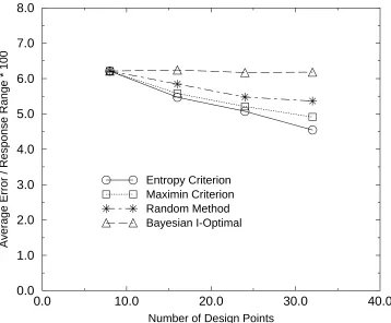
than the one with 243 evaluations.

In the same way, similar conclusions can be drawn for polynomial models. The only difference is that the piecewise polynomial model with 243 evaluations is much better that the polynomial model with 32 evaluations. When the number of evaluations is small (<= 32), there is no significant difference between the polynomial models and the MARS model. However, when the number of evaluations is increased and the piecewise linear model is used, the polynomial model is better than the MARS model, especially with 243 evaluations.

The single linear model with 3125 evaluations is also generated (listed in tables but not plotted in figures). The accuracy is almost the same as any other single polynomial model.

Among all the four measures, the ERMSE at design points is not important because those errors will be compensated by the second term of the interpolation model as in the Equation 3.3.

From the other three measures for all models with design points up to 243, the piecewise linear model (PLM) has the smallest maximum absolute error51.385, the smallest ERMSE7.2887, and the smallest error at the maximum response0.0000. Although the error at the maximum response is meaningless because that point is included in 243 design points of PLM, it seems that the apparent choice should still be the piecewise linear model if the computational cost of the finite element model is negligible. But because the design of experiment for the PLM is a 3-level full factorial design with3n _{= 243}_{design points, the PLM with}₂n _{= 32} _{models is equivalent to dividing the} DVS equally into2nsub-DVS and building one linear model for each sub-DVS. And if the cost of the computer experiment is not negligible, the number of design points should also be taken into consideration. For a ten-dimensional DVS (n = 10), the PLM needs3n = 59049design points, but the linear model or quadratic model will work with only 27 design points. So the PLM is not a feasible choice in practice. Actually, the good performance of the PLM only shows the effect of reducing the size or volume of the DVS to be exploited.

For all other models, the three measures only differ slightly. The high-order polynomial model and the MARS model, which includes nonlinear interactions, are not so appealing because these complex models could not outperform the simpler models. Because the two-way interactions can be transformed into second-order terms of main factors,

x0₁·x0₂= (x₁−x₂)·(x₁+x₂) =x2₁−x2₂, ifx0₁= (4 x₁−x₂)andx0₂ = (4 x₁+x₂)

(49)

design, otherwise it is equivalent to a linear model with interaction terms under another coordinate system. The linear model will work well with a Resolution III fractional factorial design, which consists at most of half the design points needed for a balanced quadratic model.

Finally, based on a balance of all of these considerations, the linear model 3.8 is chosen as the base function.

3.6 Criteria for Sampling Design Points with a priori Information

Once the base functions and the cov structure of the interpolation model are decided, the metamodel can be built with a set of design points and the corresponding responses. When building the first metamodel at the first stage, in general it is not possible to assume any specific knowledge about the objective function because of the wide range of functions in engineering systems. So the initial design points are chosen by a experimental design method. After the first stage, some knowledge of the objective function is obtained from the responses at design points and the metamodel. It would be helpful if design points can be chosen based on data at previous stage or stages in order to build better metamodels.

After constructing the metamodel of theithstage, a set ofnidesign points existsSi={s1, . . . , sni}. Now some new design points {s₁₊ni, . . . , sn1+i} need to be chosen according to a sampling cri-terion, and append them to Si in order to generate the (i+ 1)th set of design points Si+1 = {s₁, . . . , sni, s1+ni, . . . , sn1+i}.

Among many sampling criteria, the maximum entropy sampling criterion has a sound basis. Lindley [33] introduced ideas from Shannon’s information theory into the area of experiment de-sign, and established a measure of the information provided by an experiment. Later Shewry and Wynn [54] defined the maximum entropy sampling criterion for the set of fixed candidate design points.

For a random processY in the design space, letT ={X₁,· · ·, XN}be the set of all possible candidate design points and corresponding responses, and S ⊂ T be the chosen design points,

S=T\Sbe the complementary set ofS. The following relation can be obtained.

Ent(Y) =Ent(S) +ES(Ent(S|S)) (3.15)

The second term of the right side is the entropy for the conditional distribution of the unsampled

(50)

because the left side, the entropy of the process, is fixed, minimizing the second term on the right side equals to maximizing the first term, which is the entropy of the chosen design points. If Y

is a Gaussian process as assumed in Section 3.2, Ent(Y)is, up to constants, log(det(Cov(Y))). So the maximum entropy sampling criterion becomes to maximize the determinant of the posterior correlation matrix which is

D= [Cov(Y(si), Y(sj))]1≤i≤ni+1,1≤j≤ni+1 (3.16)

The conclusions above are based on the assumption of finite set of possible design points. By the different use of the entropy formula, Wynn et al. proved the same conclusions while loosening the condition of discrete design points [53].

Also there are several variations of the maximum entropy criterion. If the first term in Equa-tion 3.3 is a constant, then the criterion becomes maximizingdet(D)·kD−1k [3]. If there is random error whose variance tends to∞in the model, the criterion becomes minimizingkDk [36]. The operatork · kin above criteria is the sum of all entries in the covariance matrix.

Johnson et al. [22] proposed the maximin distance design. For the Gaussian process with the covariance structure as in Equation 3.4, the maximin distance design is asymptotically equivalent to the maximum entropy design under some conditions [22]. For any subset S ofT containing n

design points,S◦is a maximin distance design if

max

S s,smin0∈S d(s, s

0_{) = min}

s,s0∈S◦ d(s, s

0₎ _(3.17)

whered(s, s0)is a distance function of a pair of design points. For the model in Section 3.2,d(s, s0) is the m-dimensional Euclidean distance. By maximizing the minimum distance between design points, this criterion tries to reduce the redundancy among design points.

Johnson et al. also proposed the the minimax distance design in a similar way [22]. For any subsetSofT containingndesign points, we callS∗a minimax distance design if

min

S maxt∈T d(t, S) = maxt∈T d(t, S

∗₎ _(3.18)

whered(t, S) = mins∈Sd(t, s).

Set mapping in the method of imprecision

Acknowledgements

Abstract

Contents

List of Figures

List of Tables

Chapter 1

Introduction

x

9

x

10

2

3

4

(0,2)

(-0.05,0)

(0,-2)

(0.05,0)

1

(0.05,-1.36)

center point

1.1

Organization of Thesis

K

B

78,000

3

78,500

77,500

13,200

13,300

13,400

1

K

T

center point

2

4

(0.05,-1.36)

Chapter 2

The Basics of the Method of Imprecision

2.1

The Basic Concepts

2.2

The Aggregation Functions

2.3

Weights of Preferences

2.4

Weighted Means

2.5

Hierarchical Aggregation

2.6

Summary

Chapter 3

Metamodels for the Mapping between DVS and PVS

3.1

Approximation or Interpolation

3.2

Interpolation Model

3.3

Experimental Design

3.4

Base Functions

3.5

Method for Selection of the Base Functions

3.6

Criteria for Sampling Design Points with a priori Information

₉

₁₀

_B

_T