http://www.sciencepublishinggroup.com/j/cmr doi: 10.11648/j.cmr.20170606.14
ISSN: 2326-9049 (Print); ISSN: 2326-9057 (Online)
Intelligent Classification Models for Gestational Diabetes:
Comparative Study
Eboka Andrew Okonji, Okobah Ifeoma Patricia, Oluwatoyin Yerokun Mary
Department of Computer Education, Federal College of Education Technical, Lagos, Nigeria
Email address:
[email protected] (E. A. Okonji), [email protected] (O. I. Patricia), [email protected] (O. Y. Mary)
To cite this article:
Eboka Andrew Okonji, Okobah Ifeoma Patricia, Oluwatoyin Yerokun Mary. Intelligent Classification Models for Gestational Diabetes: Comparative Study. Clinical Medicine Research. Vol. 6, No. 6, 2017, pp. 192-200. doi: 10.11648/j.cmr.20170606.14
Received: April 5, 2017; Accepted: October 8, 2017; Published: December 7, 2017
Abstract:
Diabetes mellitus, a metabolic disease that features high glucose levels in the body with the inability of the body to secret enough insulin to breakdown glucose, or such a body is resistant to the effects of insulin. Nigeria and other nations of the world have become aware of the inherent threats to life of gestational diabetes in mothers with or without previous cases and its tendencies to metamorphose into Type-II. Our study presents a comparative study of classification models using both the supervised (K-nearest neighborhood and Quadratic Discriminant Analysis) and unsupervised (Profile Hidden Markov Model and Memetic algorithm) methods – which aims at early detection as well as improve early diagnosis via data-mining tools. Adopted dataset is split into: training (in some cases, retraining) and testing to aid model validation. Results show that age, obesity and family ties to the second degree, environmental conditions of inhabitance are critical factors that can increase likelihood. Gestational diabetes in mothers with or without previous cases were confirmed if: (a) history of babies weighing > 4.5kg at birth, (b) insulin resistance with polycystic ovary syndrome, and (c) abnormal tolerance to insulin. Also, PHMM outperforms Memetic algorithm in some cases; while memetic algorithm outperforms PHMM in some cases.Keywords:
Diabetes, Gestational, Fuzzy, Classifiers, Diab Care, Mellitus, Memetic Algorithm1. Introduction
Diabetes mellitus has now become a general chronic disease that affects about 6% of the global population – so that its avoidance and early detection for effective treatment has become imperative and undoubtedly a critical task for health and economic issue in 21st century (Khashei et al, 2012). Diabetes is a metabolic disease that is characterized by the presence of hyperglycemia or high blood glucose. This result from the body’s inability to secrets enough insulin that the body requires for glucose processing as a byproduct of the carbohydrate that we eat, or that the body is resistant to the effects of insulin. Thus, the reason why it is popularly named the silentkiller. Glucose, as a main source of energy for cells that makes up the muscles and other tissues, is produced from the food we eat and in our liver. Sugar (or glucose) is absorbed in the bloodstream and enters into a cell by the help of insulin. Liver stores glucose as glycogen so that if glucose becomes low, the liver reconverts the stored glycogen into glucose to normalize the glucose level (Ojugo et al, 2015). Diabetes is a diagnosis from glycemia that is associated with microvascular
disease (Goldenberg and Punthakee, 2013).
Diabetes is associated with range of complications such as risk of blindness, blood pressure, heart and kidney diseases, and nerve damage to mention a few (Temurtas et al, 2009; Ojugo et al, 2016). Its early detection is extremely difficult by experienced physicians, and thus – led to a continued quest for methods to effectively and precisely classify the disease. Khashei et al (2013). Ojugo et al (2015) Various models have been used for its early detection and identification to include: (a) supervised classification in which its input variables for the diagnosis are known), and (b) unsupervised classification in which the variables used for diagnosis and classification are
unknown). In both instance, a critical feat in selecting the appropriate classification model to use is, its accuracy and precision ability in classifying the task at hand.
1.1. Types of Diabetes
Diabetes is generally classified into (Ojugo et al, 2015):
a. Type-1 is a chronic condition/state, in which the
threats. Type-1 has no cure as it is insulin-dependent and its causes are unknown. Its symptoms include: blurred vision, extreme hunger, increased thirst, irritability, incessant urination, fatigue, mood changes, unintended weight loss, vaginal yeast infection (in females), bedwetting etc; Some of its known risk factors include: genetics, family history, age, geography, exposure to bacteria and Epstein-Barr virus in environ, early exposure to cow milk, low vitamin D, early or late introduction to cereal/gluten in baby diet, intake of nitrate-contaminated water, mothers with preeclampsia at pregnancy and babies born with jaundice (American Diabetes Association, 2009; Ojugo et al 2016).
b.Type 2 (adult onset or noninsulin-dependent) diabetes is
a chronic condition that affects how the body metabolizes sugar (glucose). It often develops slowly since the body either resists the effects of insulin as produced or does not produce enough insulin to maintain a normal glucose level. Though common in adults, this type is increasingly common now to children with obesity issues. While, there is also no cure for type-2, it can however be managed through proper eating habits, exercising, maintaining a healthy weight and sometimes, diabetes medications or insulin therapy. Its symptoms are increased thirst/hunger, weight loss, frequent urination, fatigue, blurred vision, acanthosis nigricians (areas of darkened skin) amongst others (Peter, 2012; Canadian Diabetes Association, 2014; Ojugo et al, 2016). Chinenye and Young (2011) Type-2 diabetes has asymptomatic preclinical phase which is not benign and thus, underscores the need for primary prevention and population screening in order to achieve early diagnosis and treatment. The prevalence of undiagnosed diabetes is been found to range from 4.76% of outpatients attending a family practice clinic, to as high as 18.9% in Nigeria. And such prevalence is higher by 68% in persons of higher socioeconomic status.
c. Gestational diabetes represents glucose intolerance from
onset, and is first recognized during pregnancy. It causes high blood sugar that can affect pregnancy and the baby’s health, though the blood sugar usually returns to normalcy soon after delivery. A patient with gestational diabetes is at the risk of type-2 diabetes with each pregnancy and it does not cause any noticeable signs (Canadian Diabetes Association, 2014; Chinenye and Young, 2011).
1.2. Gestational Diabetes Diagnosis: The Nigerian Scenario
Gestational Diabetes Mellitus (GDM) is defined as disorder of glucose tolerance occurring first in pregnancy in mothers – whereas, some experts have viewed and believe GDM to be of same entity with Type-II – wherein the former constitutes the early signs and manifestation of the latter. GDM is endemic around the world and its prevalence differs from one region to another. Its risk factors include: family history of DM in first-degree relatives, child bearing with congenital anomaly, baby weighs more than 4000g or more, dying of unknown
causes at birth, obesity, age greater than 35years amongst other. Various techniques are available to diagnose GDM as to what to test, when to perform such tests and what method is best. Most authors continually favor the early weeks of third trimester (between 26-to28 weeks) of pregnancy as best time to screen for GDM. Its investigations can be divided into
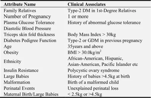
screening and definitive tests (Adebisi et al, 2012). The risk factors can be seen in the table 1.
It is a known fact that type-II diabetes has an asymptomatic preclinical phase that is not benign and underscores the need for primary prevention and population screening in order to achieve early diagnosis and treatment. The prevalence of undiagnosed diabetes has been found to range from 4.76% in one study of outpatients attending a family practice clinic to as high as 18.9% in another study. Prevalence of diabetes was found to be higher by as much as 68% in persons of a higher socioeconomic status were earlier studies had reported lower prevalence rates for undiagnosed diabetes in the population – whereas Nyenwe et al (2003) reported a 2.8% rate of disease in Port Harcourt and 1.7% in Lagos metropolis in 1988. Arije et al (2007) concurred with a satisfactory systolic and diastolic blood pressure control was obtained in only 38.5% and 42.2% of some Nigerian patients attending a tertiary health facility, respectively.
Diabcare Nigeria in 2008 took a sample study conducted across 7-tertiary health centers in Nigeria with the objective of assessing clinical and laboratory profile, evaluating the quality of care of Nigerian diabetics with a view to planning improved diabetes care. Clinical parameters studied include: diabetes types, anthropometry, blood pressure, chronic complications of diabetes and treatment types. Laboratory data assessed include: fasting plasma glucose (FPG), 2 Hour post-prandial (2-HrPP), glycated haemoglobin (HbA1c), urinalysis, serum lipids, electrolytes, urea and creatinine. A total of 531 patients, 209(39.4%) males and 322(60.6%) females enrolled. Results indicate the mean age of the patients was 57.1±12.3years with mean duration of diabetes of 8.8±6.6years. A majority (95.4%) had Type-II 2 diabetes compared to Type-I (4.6%) using a p < 0.001 significance. Mean FPG, 2-HrPP glucose and HbA1c were noted at 8.1±3.9mmol/L, 10.6±4.6mmol/L and 8.3±2.2% respectively. Only 170 (i.e. 32.4%) male and 100 (i.e. 20.4%) female patients achieved the ADA and IDF glycaemic targets respectively. About 72.8% patients did not practice self-monitoring of blood glucose and hypertension is found in 322 (i.e. 60.9%) patients, with a mean systolic BP of 142.0±23.7mmHg and mean diastolic BP of 80.7±12.7mmHg (Chinenye and Young, 2011).
test as a little above 40% of these cases are missed. Also, no screening method is consistently reliable. Thus, the rationale for this study to early detect GDM in mother as maternal mortality has been seen to be on increase (Ojugo et al, 2015). The idea is to advance for early diagnosis and detection of GDM and Type-II in mothers (with or without previous cases) using intelligent classification (supervised and unsupervised) model. This task seeks to allow model to propagate observed data as input – as the model seeks to uncover the underlying probability of data feats of interest, even with the data fed in as input consisting of ambiguities, noise and impartial truth. The model will seek to yield an output that is guaranteed of high quality and void of ambiguities. These models, further tuned can become robust and perform quantitative processing to ensure qualitative knowledge and experience, as its new language (Ojugo et al, 2013, Heppner and Grenander, 1990).
2. Materials
2.1. Dataset Used
Table 1. Risk factor for GDM and Clinical Parameters for Encoding Dataset Schema Used.
Attribute Name Clinical Associates
Family Relatives Type-2 DM in 1st-Degree Relatives
Number of Pregnancy 1 or more
Plasma Glucose Tolerance History of abnormal glucose tolerance Diastolic Blood Pressure
Triceps skin fold thickness Body Mass Index > 30kg
Diabetes Pedigree Function Type-2 or GDM in previous pregnancy Age 35years and above
Obesity BMI > 30.0kg/m2
Ethnicity African-American, Hispanic, Asian-American, Pacific Islander etc Insulin Resistance Polycystic ovary syndrome Large Babies History of babies >4.5kg at birth Malformation Birth of a malformed child Perinatal Events Unexplained perinatal loss Maternal Birth/Large Babies < 2.5kg or >4.5kg
Some statistical information of attributes is given in Table 1.
The data set consists of 768 samples, about two third of which have negative diabetes diagnosis and one third with a positive diagnosis. The data set is randomly split into equal size of training and test sets of 384 samples each.
2.2. Statement of Problem
The problem statements are as follows:
1.Being a silent killer makes its early detection, critical and imperative – as an unchecked scenario leads to increased maternal mortality. The use of supervised diagnosis is becoming redundant as it sometimes yields inconclusive
results due to unknown inputs. Studies show conditions
not even related to diabetes (but with symptoms similar or mimics type of diabetes class). Such classification results in increased rate of false-positives (unclassified
symptom) and true-negatives (to classify symptom as diabetes when it is not). Proposed model seek to
effectively group data into definitive classes of diabetes
(GDM) via evolutionary unsupervised models that
employs predictive data-mining rules and reinforcement learning (Section III).
2.Hybrid models have been employed in many studies on
diabetes. However, there are tradeoffs to be made as well as conflicts that needs to be resolved such as the conflict imposed on the model by the various underlying statistical dependencies that exist between the various heuristic method being adopted by the hybrid as well as the conflict imposed on the hybrid model by the dataset used. The proposed model resolves this (Section III) via the creation of profiles that assigns scores to rules that effectively classifies data into various types or classes of diabetes.
3.Many datasets often consist of ambiguities, imprecision,
noise and impartial truth that must be resolved via robust search. Also, speed constraint that often gets such solution trapped at local minima (resolved in Section III).
4.Parameter(s) selection can be quite a daunting task when
searching a solution space for a complete and optimized solution that will aid effective and efficient classification in a certain domain. Careful selection is required so that the system does not result in model over-fitting of data as well as overtraining cum over-parameterization (resolved in Section III) as the model seeks to discover underlying probability of the data feat(s) of interest.
3. Intelligent Proposed Model
We seek to compare various supervised model (LDA and Support Vector Machine) against the unsupervised models (Hidden Markov Model and Fuzzy Genetic Algorithm Trained Neural Net Model) to measure their comparative performance.
3.1. Linear Discriminant Analysis (LDA)
LDA is a very simple and effective supervised classification method with wide range of applications. Its basic theory is to
classify compounds (rules) dividing n‐dimensional descriptor
space into two regions separated by a hyper‐plane that is defined by linear discriminant function. Discriminant analysis generally transforms classification tasks into functions that partitions data into classes; Thus, reducing the problem to an identification of a function. The focus of discriminant analysis is to determine this functional form (assumed to be linear) and estimate its coefficients. LDA was first introduced in 1936 by Ronald Aylmer Fisher and his LDA function works by finding the mean of a set of attributes for each class, and using the mean of these means as boundary. The function achieves this by projecting attribute points onto the vector that maximally separates their class means and minimizes their within-class variance as expressed in Eq. 1 as follows:
where X is vector of the observed values, Xi (i = 1, 2…) is the
mean of values for each group, S is sample covariance matrix
of all variables, and c is cost function. If the misclassification cost of each group is considered equal, then c = 0. A member is classified into one group if the result of the equation is greater than c (or = 0), and into the other if it less than c (or = 0). A result that equals c (set to 0) indicates such a sample cannot be classified into either class, based on the features used by the analysis. LDA function distinguishes between two classes – if a data set has more than two classes, the process
must be broken down into multiple two‐class problems. The
LDA function is found for each class versus all samples that were not of that class (one‐versus‐all). Final class membership for each sample is determined by LDA function that produced the highest value and is optimal when variables are normally distributed with equal covariance matrices. In this case, the LDA function is in same direction as Bayes optimal classifier (Billings and Lee, 2002), and it performs well on moderate sample sizes in comparison to more complex method (Ghiassi and Burnley, 2010). Its mathematical function is simple and requires nothing more complicated than matrix arithmetic. The assumption of linearity in the class boundary, however, limits the scope of application for linear discriminant analysis. Real‐world data frequently cannot be separated by linear boundary. When boundaries are nonlinear, the performance of the linear discriminant may be inferior to other classification methods. Thus, to curb this – we adopt a decimal encoding of the data to give us a semblance of linear, continuous boundaries.
3.2. K-Nearest Neighbourhood (KNN)
The K‐nearest neighbour (KNN) model is a well-known
supervised learning algorithm for pattern recognition that first introduced by Fix and Hodges in 1951, and is still one of the most popular nonparametric models for classification
problems (Fix and Hodges 1951; 1952). K‐nearest
neighbour assumes that observations, which are close together, are likely to have the same classification. The probability that a point x belongs to a class can be estimated by the proportion of training points in a specified neighbourhood of x that belong to that class. The point may either be classified by majority vote or by a similarity
degree sum of the specified number (k) of nearest points. In
majority voting, the number of points in the neighbourhood belonging to each class is counted, and the class to which the highest proportion of points belongs is the most likely classification of x. The similarity degree sum calculates a similarity score for each class based on the K‐nearest points and classifies x into the class with the highest similarity score. Its lower sensitivity to outliers allow majority voting to be commonly used other than the similarity degree sum (Chaovalitwongse, 2007). We use majority voting for the data sets to determine which points belongs to
neighbourhood so that distances from x to all points in the
training set must be calculated. Any distance function that specifies which of two points is closer to the sample point could be employed (Fix and Hodges, 1951). The most
common distance metric used in K-nearest neighbour is the
Euclidean distance (Viaene, 2002). The Euclidean distance between each test point ft and training set point fs, each with
n attributes, is calculated via Eq. 2:
= − + − … + − (2)
In general the following steps are performed for the
K-nearest neighbour model (Yildiz et al., 2008): (a) chosen of
k value, (b) distance calculation, (c) distance sort in ascending order, (d) finding k class values, (e) finding dominant class.
A challenge in K‐nearest neighbour is to determine optimal size of k that acts as a smoothing parameter. A small k is not sufficient to accurately estimate population proportions around test point. A larger k will result in less variance in probability estimates (but for risk of introducing more bias). K
should be large enough to minimize probability of a non‐ Bayes decision, and small enough that all the points included, gives an accurate estimate of the true class. Enas and Choi (1986) found optimal value k depends on sample size and covariance structures in each population and on the proportions for each population in the total sample. For cases where the differences both in covariance matrices and between sample proportions are both small or both large, it is found that optimal k is N3/8 (N is number of samples in the training set). If and when there is a large difference between covariance matrices, and a small difference between sample proportions (or vice-versa), the optimal value k is determined by N2/8(Enas and Choi, 1986).
This model presents several merits (Berrueta et al., 2007) in that: (a) its mathematical simplicity does not prevent it from achieving classification results as good as (or even better than) other more complex pattern recognition techniques, (b) it is free from statistical assumptions, (c) its effectiveness does not depend on the space distribution of the classes, and (d) when the boundaries between classes are not hyper‐linear or hyper‐ conic, K-nearest neighbour performs better than LDA.
However, Enas and Choi (1986) found that LDA performs
slightly better than K‐nearest neighbour when the population
covariance matrices are equal, a condition that suggests linear boundary. As the differences in covariance matrices increases, K‐nearest neighbour performs increasingly better than the linear discriminant function. However, despite these merits of the model, the demerits of the K-nearest neighbour models includes that model does not work well if large differences are present in samples in each class. K‐nearest neighbour provides poor information about the structure of the classes and of the relative importance of each variable in the classification. Laos, it does not allow a graphical representation of the results, and in the case of large number of samples, computation become
excessively slow. In addition, K‐nearest model requires more
3.3. Bayesian Profile Hidden Markov Model (PHMM)
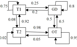
Ojugo et al (2016) describes the Hidden Markov model as used in examination scheduling. Adapted to GDM diabetes classification problem, probability from one transition state to another is as in figure 1. The PHMM is a double embedded chain that models complex stochastic processes (Bhusai and Patil, 2011; Masoumeh, Seeja, and Afshar, 2012). Markov process is a chain of state probabilities associated to each transition between states. In n-order Markov, its transition probabilities depend on current and n-1 previous states. A HMM process determines the state generated for each state observation in a series (output sequence). For GDM diabetes analysis, a rule not accepted by the trained HMM, yields high probability of either a false-positive or true-negative result (Ojugo et al, 2016). Traditional HMM scores data via clustering based on profile values. Probabilities of initial set of rules are sampled – then classified into GDM or non-GDM class. HMM maintains a log in memory to help reduce high true-negatives (rules of symptoms with semblance of diabetic feats) and high-false positives (unclassified rules for diabetes). Thus, our HMM is initially trained to assimilate normal behaviour of the various types or diabetes class/types. It then creates a profile of the rules, classifying them into type-1, type-2, gestational and other profile ranges were possible (Tripathi and Pavaskar, 2012; Ojugo et al, 2016).
Figure 1. Actual State Transition with P(x)
The Profile HMM as a variant of HMM, proffers solution to the fundamental problems of the HMM by: (a) makes explicit use of positional (alignment) data contained in observations or sequences, and (b) allows null transitions, where necessary so that the model can match sequences that includes insertion and deletions (Ojugo et al, 2014). Used in GDM early detection, O is each rules contained therein to define the various symptoms of GDM diabetes type, T is time it takes each rule to classify data input, N is number of unclassified rules and those with symptom semblance that results in false-alarm rates, M is the number of rules accurately classified, π is the initial state or starting rule, A is state transition probability matrix, aij is the probability of a transition from a state i to another state j, B contains the N probability distributions for the codes in the knowledgebase from where profiles have been created (one rule for each state of the process); while HMM λ = (A, B, π). Though, parameters for HMM details are incomplete as above; But, the general idea is still intact (Ojugo et al, 2016).
Figure 2. PHMM with 3-Match States. We can also align multiple codes (data) rules as sequence
with significant relations. Its output sequence determines if an unknown code is related to sequence belonging to either of the diabetes (type class) or its variant (or those not) contained in the Bayesian net. We then use the profile HMM to score codes and make decision. Circles are delete state that detects rules as classified into GDM-diabetes types, rectangle are insert states that allows us to accurately classify rules of symptoms that have been previously unclassified inputs into a class type and consequently, update knowledgebase of the classified
false-positives and true-negatives; diamonds are matched
states that accurately classifies rules of symptoms into variants of similar symptom or unclassified rules, as in standard HMM (Ojugo et al, 2014; 2016). Delete and insert are emission states
= !"#
$"# + log () ) exp - . − 1 0 + (1 ) exp
-2 . − 1 0 + (3 ) exp - 4 . − 1 0 (3)
2 = 2!"#
$"# + log () 1 exp - . − 1 0 + (1 1 exp
-2 . − 1 0 + (3 1 exp - 4 . − 1 0 (4)
4 = 5og () 3 exp - . 0 + (1 3 exp - 2 . 0 + (3 3 exp - 4 . 0 (5)
3.4. Fuzzy Genetic Algorithm Trained Neural Network Model
The GANN is initialized with if-then rules. Individual fitness is computed as 30-individual are selected via the tournament
method to determines new pool and individuals for mating. Crossover and mutation is applied to help net learn dynamic and non-linear feats in the dataset and feats of interest using a multi-point crossover. As new parents contribute to yield new individuals whose genetic makeup is combination of both parents, mutation is reapplied and are allocated new random values that still conforms to belief space. Number of mutation applied depends on how far CGA is progressed on the network (how fit is the fittest individual in the pool), which equals fitness of the fittest individual divided by 2. New individuals replace old with low fitness so as to create a new pool. Process continues until individual with a fitness value of 0 is found –
indicating solution is reached (Ojugo et al, 2013).
Initialization/selection via ANN ensures that first 3-beliefs are met; mutation ensures fourth belief is met. Its influence function influences how many mutations take place, and the knowledge of solution (how close its solution is) has direct impact on how algorithm is processed. Algorithm stops when best individual has fitness of 0 (Dawson and Wilby 2001). Model stops if stop criterion is met. GANN utilizes number of epochs to determine stop criterion.
4. Result Findings and Discussion
4.1. Model Performance
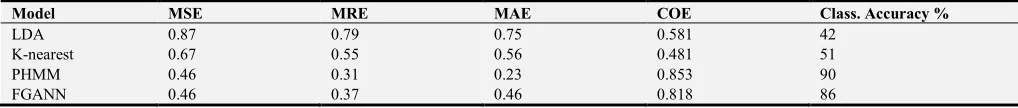
Ojugo et al (2013) Performance is evaluated via computed values: mean square error, mean absolute error, mean relative error and coefficient efficiency as thus:
Table 2. Model Convergence Performance Evaluation.
Model MSE MRE MAE COE Class. Accuracy %
LDA 0.87 0.79 0.75 0.581 42
K-nearest 0.67 0.55 0.56 0.481 51
PHMM 0.46 0.31 0.23 0.853 90
FGANN 0.46 0.37 0.46 0.818 86
Table 3. Clinical Parameters and Association.
No Attribute Name µ σ
1 Number of Pregnancy 3.8 3.4
2 Plasma Glucose (2 Hours) 121 32 3 Diastolic Blood Pressure 69.1 19.4 4 Triceps skin fold thickness 20.5 16.0 5 Two Hour Serum Insulin 79.8 115.2 6 Body Mass Index 32.0 7.9 7 Diabetes Pedigree Function 0.5 0.3
8 Age 33.2 11.8
4.2. Result Findings and Discussion
To measure their effectiveness and classification accuracy, we adopt the misclassification rate of each model as well as its corresponding improvement percentages of the proposed model in comparison with those of other classification models for the diabetes data in both training and test data sets as summarized in Table 2 and Table 3, respectively. The equations for the misclassification rate and its improvement percentage of the unsupervised (B) model against those of the supervised (A) model, is respectively calculated as follows:
).6 5(66. . (7. 8 9(7: )9 = ;<.<> 2 ?<@@ ? 4ABC < A;<.<> DBEFG (6)
1HIJ K:H:87 L:J :87( : = M NM NM O P 100 (7)
Table 4. Misclassification Rate of Each model.
Model Classification Errors
Training Data Testing Data
LDA 36.6% 34.9%
K-Nearest Neighbourhood 43.4% 39.7%
PHMM 18.7% 15.8%
FGANN 19.3% 18.3%
Table 5. Improvement Percentage.
Model Improvement %
Training Data Testing Data
LDA 45.83% 41.16%
K-Nearest Neighbourhood 41.79% 43.09%
PHMM 78.78% 76.33%
FGANN 69.30% 69.91%
Tables 4 and 5 shows unsupervised model has lowest error
different attributes, all attributes are scaled by their z‐scores
before using K‐nearest neighbour model in tandem with
Antal et al (2003). 4.3. Related Study
Barakat et al (2010) adopts SVM by using an additional intelligent module to transform black-box SVM model to an intelligent SVM's diagnostic model with adaptive results that provides a potential model for diabetes prediction. Its logical rule set generated had prediction accuracy of 94%, sensitivity of 93%, and specificity of 94%. Extracted rules are medically sound and agree with outcome of relevant medical studies.
Khasei et al (2012) adopted a feed-forward
multi-perceptron network in their study. Such networks must be expanded and extended to represent complex dynamic patterns and/or cases such as this, since it treats all data as new – so that previous data signals do not help to identify data feats of interest, even if such observed datasets exhibits temporal dependence. Consequently, this has practical implementation difficulty as large nets are not easily implemented. However,
Jordan net overcomes such difficulty via use of its internal feedbacks that also makes it appropriately suitable for such dynamic, non-linear and complex tasks as its output unit is fed-back as input into its hidden unit with a time delay, so that its outputs at time t−1, is also input at time t. Also, Ojugo et al (2015).
The rationale for the choice of techniques adopted is to compare between: (a) supervised versus unsupervised model, (b) seek a measure to lay claims to superiority of a class of models (supervised/unsupervised) over the other for the task at hand, (c) compare clustering (profile) versus hill-climbing heuristic, and (d) measure the convergence behavior and other statistic between PHMM and FGANN. On this latter, it was observed that PHMM converged after 253-iterations; while FGANN converged after 213-iterations. And though, FGANN is significantly better and outperforms PHMM in some tasks; while PHMM have been found to outperform FGANN in classification accuracy.
We note, model’s speed is traded-off for greater accuracy of classification, more number of rule set generated to update the knowledge database for optimality and greater functionality.
5. Conclusion and Recommendations
As for GDM, its risk factors are many and must be assessed regularly in all pregnant women. Placental mass and hormonal changes during pregnancy may contribute to the pathogenesis of GDM. Insidious onset of most cases of GDM necessitates a diligent search and screening, and while, we advise that RBG, FBG, and OGTT to be used in GDM diagnosis (as agreed by Opta and Nzeribe, 2013). A significant number of cases of GDM in pregnancy require insulin for treatment. There is now increasing evidence, that sulphonylureas and metformin are safe in pregnancy. The management and follow-up of GDM is for life.
Furthermore, our study employed supervised (K-nearest
neighbourhood/LDA) and unsupervised (PHMM/FGANN as
benchmark for classification of GDM) models – and consists of 5-phases: (a) train models with available data, (b) determine minimal fuzziness via the obtained weights and same criterion, (c) delete outliers in data, (d) compute membership probability of output, and (e) assign output to appropriate class by largest probability. Four known intelligent classification
models: LDA, K‐nearest neighbour, PHMM and FGANN
are used to show their classification efficiency for early prognosis of GDM. The hybrid unsupervised models outperforms, and is better than K-nearest and LDA (alongside other traditional classification models).
The unsupervised models do not assume the shape of the partition, unlike the linear and quadratic discriminant analysis.
In contrast to K‐nearest neighbour model, the proposed
model does not require storage of training data. Once the model has been trained, it performs much faster than K‐ nearest neighbour does, because it does not need to iterate via individual training samples. Proposed model does not require experimentation and final selection of kernel function and a penalty parameter as is required by the support vector machines. Our proposed model solely relies on a training process in order to identify the final classifier model. Finally, the unsupervised models does not need large amount of data in order to yield accurate results.
References
[1] Adebisi, S. A., Oparinde, D. P., Olarinoye, J. K., Aboyeji, P. A and Ogunro, P. S., (2012).
[2] American Diabetes Association. Standards of Medical Care in Diabetes – 2009. Diabetes Care, 32: S13-61.
[3] Antal, P., Fannes, G., Timmerman, D., Moreau, Y., and Moor, B. D., “Bayesian applications of belief networks and multilayer perceptrons for ovarian tumor classification with rejection”, Artificial Intelligence in Medicine Vol. 29, pp. 39–60, 2003. [4] Barakat, N. H., Bradley, A. P., Barakat, M. N. H., (2010).
Intelligible support vector machines for diagnosis of diabetes mellitus, IEEE Transactions on Information Technology in Biomedicine, 14(4), pp1114-1120.
[5] Berks, G., Keyserlingk, D., Jantzeen J., Dotoli, M and Axer H. (2000). Fuzzy clustering: versatile means to explore medical database, ESIT, Aachen, Germany.
[6] Berardi, V. and Zhang, G. P., “The effect of misclassification costs on neural network classifiers”, Decision Sciences, Vol. 30, pp. 659–68, 1999.
[7] Billings, S. and Lee, K., “Nonlinear Fisher discriminant analysis using a minimum squared error cost function and the orthogonal least squares algorithm”, Neural Networks, Vol. 15, pp. 262–270, 2002.
[8] Calisir D. and Dogantekin, E., “An automatic diabetes diagnosis system based on LDA‐Wavelet Support Vector Machine Classifier”, Expert Systems with Applications, Vol. 38, pp. 8311– 8315, 2011.
[10] Caudill M., (1987). Neural Networks Primer, AI Expert, pp46-52.
[11] Chakraborty, R., (2010). Soft computingand fuzzy logic, Lecture notes 1-37, retrieved from
http://www.myreaders.info/07_fuzzy_systems.pdf
[12] Chaovalitwongse, W., “On the time series k‐nearest neighbor classification of abnormal brain activity”, IEEE Transactions on Systems, Man, and Cybernetics–Part A: Systems and Humans, Vol. 37, 2007.
[13] Charya, S., Odedra, D., Samanta, S., and Vidyarthi, S., “Computational Intelligence in Early Diabetes Diagnosis: A Review”, The Review of Diabetes Studies, Vol. 7, pp.252–262, 2010.
[14] Chinenye, S and Young, E., (2011). State of diabetes care in Nigeria: a review, The Nigerian Health Journal, 11(4), pp101-106.
[15] Coello, C., Pulido, G and Lechuga, M., (2004). Handling multiple objectives with particle swarm optimization, Proc. of Evolutionary Computing, 8, pp 256–279.
[16] Dawson, C and Wilby, R., (2001). Comparison of neural networks in river flow forecasting, J. of Hydrology and Earth Science, SRef-ID: 1607-7938/hess/2001-3-529.
[17] Edo, A. E., Edo, G. O., Ohehen, O. A., Ekhator, N. P and Ordiah, W. C., (2015). Age and diagnosis of type-2 diabetes in Benin City Nigeria, African Journal of Diabetes Medicine, Vol. 23, No. 1, Pp18-19.
[18] Enas, G. and Choi, S., (1986). Choice of the smoothing parameter and efficiency of k‐nearest neighbor, Computers and Mathematics with Applications, Vol. 12, pp. 235–244. [19] Fausett L., (1994). Fundamentals of Neural Networks, New
Jersey: Prentice Hall, pp.240.
[20] Fisher, R. A., “The use of multiple measurements in taxonomic problems”, Annals of Eugenics, Vol. 7, pp. 465–475, 1936. [21] Fix, E. and Hodges, J., “Discriminatory analysis –
Nonparametric discrimination: Consistency properties”, Project No. 21‐49‐004, Report No. 4, Contract No. AF 41(128)‐31, USAF School of Aviation, Randolph Field, Texas, 1951.
[22] Ganji M. F. and Abadeh, M. S., “A fuzzy classification system based on Ant Colony Optimization for diabetes disease diagnosis”, Expert Systems with Applications, Vol. 38, pp. 14650– 14659, 2011.
[23] Ghiassi, M. and Burnley, C., “Measuring effectiveness of a dynamic artificial neural network algorithm for classification problems”, Expert Systems with Applications, Vol. 37, pp. 3118–3128, 2010.
[24] Giles, D and Draeseke, R., (2001). Economic Model Based on Pattern recognition via fuzzy C-Means clustering algorithm, Economics Dept Working Paper, EWP0101, University of Victoria, Canada.
[25] Goldenberg, R and Punthakee, Z (2013). Definition, classification and diagnosis, prediabetes and metabolic syndrome, 37(1), S8-S11.
[26] Golub, T. R., Slonim, D. K., Tamayo, P., Huard, C., Gaasenbeek, M., Mesirov, J. P., Coller, H., Loh, M. L., Downing, J. R., Caligiuri, M. A., Bloomfield, C. D., and
Lander, E. S., “Molecular classification of cancer: class discovery and class prediction by gene expression monitoring”, Science, Vol. 286, pp. 531– 537, 1999.
[27] Guo, W. W and Xue, H., (2011) An incorporative statistic and neural approach for crop yield modelling and forecasting, Neural Computing and Applications, 21(1), pp109-117 [28] Heppner, H and Grenander, U., (1990). Stochastic non-linear
model for coordinated bird flocks, In Krasner, S (Ed.), The ubiquity of chaos pp.233–238. Washington: AAAS.
[29] Inan, G and Elif, D., (2005). Adaptive neuro-fuzzy inference system for classification of EEG using wavelet coefficient, retrieved from http://www.rorylewis.com/PDF/04
[30] Jang, J. S., (1993). Adaptive fuzzy inference systems, IEEE Transactions on Systems, Man and Cybernetics, vol.23, pp.665–685.
[31] Khashei, M., Eftekhari, S and Parvizian, J (2012). Diagnosing diabetes type-II using a soft intelligent binary classifier model, Review of Bioinformatics and Biometrics, 1(1), pp9-23. [32] Kuan, C and White, H., (1994). Artificial neural network:
econometric perspective”, Econometric Reviews, Vol.13, Pp.1-91 and Pp.139-143.
[33] Ludmila I. K. (2008), Fuzzy classifiers Scholarpedia, 3(1), pp2925.
[34] Mandic, D and Chambers, J., (2001). Recurrent Neural Networks for Prediction: Learning Algorithms, Architectures and Stability, Wiley & Sons: New York, pp56-90.
[35] Menezes, A. C., Pinheiro, P. R., Pinheiro, M. C. D., Pequeno, T., (2012). Towards the applied hybrid model in decision making: support the early diagnosis of type-2 diabetes, [online] http://www.researchgate.net/publication/262166315
[36] Minns, A., (1998). Artificial neural networks as sub-symbolic process descriptors, published PhD Thesis, Balkema, Rotterdam, Netherlands.
[37] Nascimento L., (1991). Comparative Genomus of two Leptospira interrogans Serovirs,
http://jb.asm.org/cgi/content/full/186/7/2164
[38] Ojugo, A. A, (2012). Artificial neural networks gravitational search algorithm for rainfall runoff modeling in hydrology, unpublished PhD Thesis, CS Department: Ebonyi State University Abakiliki, Nigeria.
[39] Ojugo, A., Eboka, A., Okonta, E., Yoro, R and Aghware, F., (2012). GA rule-based intrusion detection system, Journal of Computing and Information Systems, 3(8), pp 1182-1194. [40] Ojugo, A. A., Emudianughe, J., Yoro, R. E., Okonta, E. O and
Eboka, A., (2013). Hybrid neural network gravitational search algorithm for rainfall runoff modeling, Progress in Intelligence Computing and Application, 2(1), doi: 10.4156/pica.vol2.issue1.2, pp22–33.
[41] Ojugo, A. A., Ben-Iwhiwhu, E., Kekeje, D. O., Yerokun, M. O and Iyawa, I. J. B., (2014). Malware propagation on time varying network, Int. J. Modern Edu. Comp. Sci., 8, pp25–33. [42] Ojugo, A. A., Allenotor, D., Oyemade, D. A., Yoro, R. E and
[43] Ojugo, A. A, A. O. Eboka., R. E. Yoro., M. O. Yerokun., F. N. Efozia., (2015). Hybrid model for early diabetes diagnosis, Mathematics and Computers in Science and Industry, Series 50, Pp 176-182, ISBN: 978-1-61804-327-6.
[44] Ojugo, A. A., Allenotor, D., Oyemade, D. A., Yoro, R. E and Anujeonye, C. N., (2015): Immunization Model for Ebola Virus in Rural Sierra-Leone, African Journal of Computing & ICTs. Vol 8, No. 1, Issue 2, Pp 1-10.
[45] Ojugo, A. A., Allenotor, D., Oyemade, D. A., Longe, O. B and Anujeonye, C. N., (2015): Comparative stochastic study for credit-card fraud detection models, African Journal of Computing & ICTs. Vol 8, No. 1, Issue 1. Pp 15-24.
[46] Oputa, R. N and Nzeribe, E. A., (2013). Gestational diabetes mellitus: a clinical challenge in Africa, African Journal of Diabetes Medicine, Vol. 21, No. 2, pp 29–31.
[47] Perez, M and Marwala, T., (2011). Stochastic optimization approaches for solving Sudoku, IEEE Transaction on Evol. Comp., pp.256–279.
[48] Peter, S., (2014). An analytical study on early diabetes and classification of diabetes mellitus, Bonfring International Journal of Data Mining, Vol. 4, No. 2, Pp 7–11.
[49] Reynolds, R., (1994). Introduction to cultural algorithms, Transaction on Evolutionary Programming (IEEE), pp.131-139.
[50] Ursem, R., Krink, T., Jensen, M. and Michalewicz, Z., (2002). Analysis and modeling of controls in dynamic systems. IEEE Transaction on Memetic Systems and Evolutionary Computing, 6(4), pp.378-389.