Batch-to-Batch Iterative Learning Control for End-Point Qualities Based on Kernel Principal Component Regression Model

Batch-to-Batch Iterative Learning Control for

End-Point Qualities Based on Kernel Principal

Component Regression Model

Ganping Li

School of Information Engineering, Nanchang University, Nanchang City, P. R. China Email: [email protected]

Abstract—A batch-to-batch model-based iterative learning control (ILC) strategy for the end-point product quality control in batch processes is proposed in this paper. A nonlinear model for end-point product quality is developed from process operating data using kernel principal component regression (KPCR). The ILC algorithm is derived to calculate the control policy by linearizing the KPCR model around the nominal trajectories and minimising a quadratic objective function concerning the end-point product quality. To overcome the detrimental effects of unknown process variations or disturbances, it is proposed in the paper that the KPCR model should be updated in a batchwise manner by removing the earliest batch data from the training data set and adding the latest batch data to the training data set. The ILC based on updated KPCR model shows adaptability for process variations or disturbances when applied to a simulated batch polymerization process. Comparisons between KPCR model and principal component regression (PCR) model based ILCs are also made in the simulations.

Index Terms—Iterative Learning Control, Kernel Principal Component Regression, Batch Process

I. INTRODUCTION

Batch processes are very important in the industry to manufacture the low-volume and high-value products such as biochemicals, crystals and some speciality chemicals. Generally, most agile manufacturings are realized depending on batch processes because of their flexibility in handling many products. Those factors such as shorter product life cycle and more adaptive ability of time-to-market of batch processes are competitive factors in successful factories. Because batch processes playa more and more important role in economic growth, the control of batch processes and their optimal operation have received a great deal of attention in past decades.

Batch processes have some features not found in continuous processes, such as strong nonlinearity and without steady state of the system, which make batch process be difficult to control. With the development of control theories in past decades, newly emerged nonlinear control techniques were applied to batch processes, such as differential geometric approaches [1-3], nonlinear predictive control [4][5] and generic model control (GMC)[6]. However, these approaches rely on accurate

process models. If model mismatches and disturbances exist, they may not be feasible to apply these methods for real processes. When a mechanistic model is not available or difficult to develop, data-driven model based control scheme provides a viable alternative for solving control problems associated with a nonlinear batch process [7].

Recently, a control strategy called “(ILC)” has been applied to batch process control. ILC was originally developed to improve the operation of robot manipulators under repetitive operations [8]. Since batch processes are intended to be run repeatedly, ILC can be extended to control batch processes. As far as ILC for batch process is concerned, the ILC is employed to track a desired trajectory or improve the product qualities batch-to-batch by feeding the previous output error back to the present batch, so that the output converges to the desired trajectory or product qualities. Such a kind of ILCs is referred as batch-to-batch ILC. Most ILC strategies are based on models, such as system inversion [9] or model predictive control (MPC) [10-12]. Since the development and validation of an accurate mechanistic model are very hard and the remaining uncertainties may still be high, data-driven based empirical model, on the other hand, have the advantages of ease in use. Thus empirical model-based ILC approaches are developed very fast in recent years. Among them, different ANNs were used in batch-to-batch ILC design due to their non-linear regression abilities [13-15].

disturbances of batch processes, to design a more adaptive ILC scheme is still of great importance. Because KPCA has showed good advantage of capturing process dynamics, thus KPCA can be incorporated into ILC design to achieve more adaptive control.

In this article, a batch-to-batch ILC strategy based on KPCR model is proposed. The training data from several normal batches are used to build the model base on the KPCR technique. Under the ILC strategy, the end-point qualities of the batch product will converge to the target value. Additionally, by updating the model batch-to-batch, the ILC can overcome the persistent batch-to-batch disturbances or process variations effectively. The ILC strategy is more adaptive than the ILC based on PCR model.

This paper is organized as follows. KPCR modeling technique is introduced in Section 2. ILC strategy based on KPCR model is proposed in Section 3, and then Section 4 gives a simulation example. Finally, the conclusions are made in Section 5.

II.KPCR

KPCR is a nonlinear extension of PCR in kernel feature subspace. Consider a nonlinear mapping

, :Rm →F

Φ x6 X. (1) whereΦ(⋅)is a nonlinear mapping function that projects sample data

x

from the input space to the high-dimensional feature space F. If the mapped data Φ( )x are centered in feature space F, that is

1

1

( ) 0

n i i

n

∑

=Φ x = , n is

the sample number, then we have the covariance matrix in F:

1

1

( ) ( )

C n T

i i i

n =

=

∑

Φ x ⋅Φ x (2)

The first step of KPCR is to perform KPCA for sample matrixX_{n m×} , which corresponds to solve the eigenvalue problem ofC:

C

l

v

=

v

(3) where

l

is the eigenvalue and

v

is the corresponding eigenvector ofC. All solutions

v

with

l

≠

0

lie in the span of Φ( ),x₁ Φ(x₂),",Φ(xn) . Equation (3) is equivalent to the following eigenvalue problem [18]:

α

K

α

nl

=

(4)

whereα [ ₁, ₂, , ]T n

α α

α

= " ,

α

_iis the coefficient vector such that

1

( )

n

i i

i

α

=

=

∑

Φ

v

x

(5)

Kis the n×nGram kernel matrix defined as:

[ ]K _ij =K_ij = Φ( ),x_i Φ(x_j) =K( ,x x_{i j})

The PC vectors can be obtained in feature space as follows:

1

( ) , ( ) ( ), ( )

n k

k k i i

i

β

α

=

= Φ =

∑

Φ Φ

x v x x x

1

ˆ ( , )

n k i i i

K

α

=

=

∑

x x (6)

where

k

is the number of PCs reserved,k =1,2,",r. ˆ

Kis the mean centered matrix ofK, ˆ

N N N N

= − − +

K K E K KE E KE (7) where

1

1

1

1

1

N

n n

n

×

⎡

⎤

⎢

⎥

= ⎢

⎥

⎢

⎥

⎣

⎦

E

"

# % #

"

. (8)

The second step of KPCR is to perform linear regression between the nonlinear principal components and the observations in feature space. The linear regression model in feature space is:

Y =Φξ+ε (9) where Yis a vector of

n

observations of an output,

Φ

is (n×m)matrix of regressors whose i-th raw is ( )_i

Φ x , ξ is a vector of regression coefficients, and

ε

is a vector of errors.

By projection of all original regressors onto the principal components, (9) can be rewritten as:

Y =

Γ

w +

ε

(10)

where Γ=ΦV is an (n×m) matrix of transformed regressors, and Vis an (m m× )matrix whose kth column is the eigenvectorVk. Define A=[

α α

1, 2,",

α

n], then

Γcan be calculated as [22]:

ˆ

Γ

=

KA

1

ˆ ( , )

n

i i

i

α

=

=

∑

K

x x

(11) The least squares estimate of the coefficient vector

w

is:

1

ˆ

=

(

T

)

− T

w

Γ Γ Γ

Y

(12)

Finally, using the first r nonlinear principal components in feature space, the KPCR model can be formulated as [23]:

1

( , )

ˆ

( )

r

k k k

y

f

c

b

β

=

=

=

∑

+

x

1 1 1

ˆ

ˆ

( , )

ˆ ( , )

r n k

k i i

k i n i i i

b

c

b

α

= = =

=

+

=

+

∑ ∑

∑

w

x x

x x

K

K

where ₁

1ˆ

{ _i r _{k i}k}n_i

k

c =

∑

₌ w

α

₌ , b is a bias term.

III.BATCH-TO-BATCH ILC FOR END-POINT QUALITY CONTROL

A. Batch-to-Batch ILC Based on Fixed KPCR Model In batch processes, the end of batch product quality generally depends on the initiate condition and the control profile, which can be formed as

0 ( )tf =F( , )

y X U (14)

where y( )t_f =[ ( ),y t_{1 f} y t₂( )_f "y_N( )]t_f is a vector of end-point product qualities at batch end time tf. X0 is

the initiate condition of the batch process and

1 2 [ , , , ]T

L

u u u

=

U " is a vector of control inputs by dividing a batch process into L time segments of equal length. The nonlinear function vector F( , )⋅ ⋅ is represented by KPCR model here based on training data of a batch process.

Based on the KPCR model formulated by (13), the optimal control policy U can be obtained by solving the following optimization problem:

min [ ( )]

J

t

_f

U

y

(15)

s.t. product quality and process constraints

Generally, there are model mismatches and disturbances in real plants which will deteriorate the performance of a batch process if present control policy are applied. To overcome this problem, an ILC strategy is used for the improvement of the performance from batch to batch in the presence of model mismatches and disturbances. The ILC strategy uses information from previous batches to improve the operation of the next batch.

The first order Taylor series expansion of (14) around a nominal control profile can be expressed as [17]:

0 1 2

1 2

ˆ ( )f F F F F L

L

t u u u

u u u

∂ ∂ ∂

= + Δ + Δ + ⋅⋅⋅ + Δ

∂ ∂ ∂

y (16)

The actual end-point product quality for the kth batch can be written as

ˆ

( )

( )

e

k

t

f

=

k

t

f

+

k

y

y

(17)

where y_k( )t_f are the actual product qualities and

ˆ ( )k tf

y are the predicted product qualities at the end of the kth batch respectively, and ek is the model

prediction error.

From (16), the prediction for the kth batch can be approximated using the first order Taylor series expansion based on the (k-1)th batch:

1

1 1

1

1 1 1

1 1 1 2 2 2 1

ˆ

( )

ˆ

( )

(

)

(

)

(

)

ˆ

( )

|

|

|

k k k k k k f k f _U

k k k k

L L

U U

L T k k f k

t

t

u

u

u

u

u

u

u

u

u

t

− − − − − − − −

∂

=

+

−

+

∂

∂

₋

_+⋅⋅⋅+

∂

₋

∂

∂

=

+ Δ

y

y

y

U

F

F

F

G

(18) where 1 2 [ ... ]

k k k k T L

u u u

ΔU = Δ Δ Δ ,

1 1 1

1 2

|

|

|

F

F

F

G

k k k

T T

k _{U U U}

L

u

−

u

−

u

−

⎡

∂

∂

∂

⎤

=

_⎢

⋅⋅⋅

_⎥

∂

∂

∂

⎣

⎦

.

The control input can be calculated employing the conventional quadratic objective function:

2 2

1

min ( )

k

T k k k d k f k _{Q R}

J ₋ t

ΔU = y −y −G ΔU + ΔU (19)

where yd is the objective value, Q is a weighting

matrix for the end state errors and R is a weighting matrix for the control effort.

For the unconstrained case, set / k 0

J

∂ ∂ΔU = , an analytical solution to the above minimization can be obtained as

1

1

(G QG R G Q) ( ( ))

k T

k k k d k tf

−

−

ΔU = + y −y (20)

1

k = k− + Δ k

U U U (21)

Kernel function K( , )x x_i is a symmetric function satisfying the Mercer’s condition. Different kernel functions can be selected to construct different KPCR model. Here we select RBF kernel function

2 2 2

( ,x x_i)=exp(− −x x_i ) / 2σ

K to build KPCR model.

The gradient of model output with respect to U and G, can be calculated as

1 ₁ 1

2 1 1 2 2 2 1 ( , ) ( ) exp( ) 2

|

|

k k n i k i i n k i k i i i c c σ σ − ₌ − − − = ∂ ∂ = = ∂ ∂ − − = − −

∑

∑

U U U U U U U U U U K F G (22)

whereGkis the gain matrix of the ILC.

data are removed from the data set and the latest batch data are added to the data set to rebuild the KPCR model. The procedure can be formulated as

( ) ( 1) 1 ( ) 1

, 1, , 1;

i i

k k

n k

k

i n

+ + +

= = −

=

X X

X U

"

(23)

and

( ) ( 1) 1 ( ) 1

, 1, , 1;

( )

i i

k k

n

k k f

i n

t + + +

= = −

=

Y Y

Y y

"

(24)

where i denotes the ith row of the data matrix which corresponds to the ith sample.

The updated KPCR model can be established using the same KPCR technique mentioned in section 2. The ILC algorithm based on the updated KPCR model can be reformulated as

1

1

[G QG R G Q] ( ( ))

k T

k k k d k tf

−

−

ΔU = + y −y (25)

whereG_kis the updated gain matrix.

IV.NUMERICAL SIMULATIONS

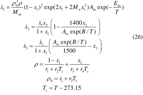
In this section, the proposed ILC method is tested through simulations for the thermally initiated bulk polymerization of styrene in a batch reactor [21]. The state equation describing the polymerization system is shown as follows:

2

2 2

0 m

1 1 1 n 1 m

m

1 2 2

2

1 w

w 1

3 3

1

1 1

1 2 c 3 4 c 0 1 2 c c

(1 ) exp(2 2 ) exp( )

1400 1

1 exp( / )

exp( / )

1 1500

1

273.15

E

x x x M x A

M T

x x x

x

x A B T

A B T

x

x x

x

x x

r r T r r T r r T

T T

ρ ρ

ρ

ρ

= − + −

⎛ ⎞

= _⎜ − _⎟

+ ⎝ ⎠

⎛ ⎞

= _⎜ − _⎟

+ ⎝ ⎠

−

= +

+ +

= + = −

(26)

where x1 is the conversion, x2=xn/xnf and 3 w/ wf

x =x x are the dimensionless number-average and weight-average chain lengths, respectively. u=T T/ refis

the dimensionless reactor temperature as control variable; Tc is the temperature in degrees Celsius;

w

A _{and B are coefficients in the relation between the}

weight-average chain lengths and the temperature obtained from experiments; Am and Em are the

frequency factor and energy of the overall monomer reaction respectively; the constants r1–r4are

density-temperature corrections; MmandMnare the monomer

molecular weight and polymer-monomer interaction parameter, respectively; and tfis the final time of the batch. The initial values of the states are x1(0)=0 , x2(0) 1= , and x3(0)=1 . The process

parameter values are given in Table 1.

To apply the ILC strategy, the sample time of the batch process is set as 20 minutes. The control profile is divided into 15 equal stages. During each stage, the control variable is kept constant. Then the control input is formed as [ ,1 2, , 15]

T

u u u

=

U " (L=15). The control outputs are the end-point qualities ( ) [ ( )1 2( ) 3( )]

T

f f f f

t = x t x t x t

y _.

In order to generate the training data to build the KPCR model, random changes with normal distribution (_{NID(0, 0.1 )}2

) are added to the nominal trajectory and data of 30 batch runs are generated as training data. Then a KPCR model is built from the training data which takesU(30 15)× as the model input and y( )(30 3)tf × as the model output. Table 2 shows the root mean squared (RMS) errors of the KPCR model outputs and the PCR model outputs. It can be seen from Table 2 that KPCR model has more accuracy than PCR model.

The ILC based on the fixed KPCR model are applied to the batch process. First, we test the ILC performance under normal condition. The ILC uses the law of (20)

TABLE I.

PARAMETER VALUES FOR THE BATCH POLYMERIZATION PROCESS

Parameter Value

Mm 104 kg/mol

Aw 0.033454

Am 4.26 × 105 m3/(kmol s)

Em 10103.5 K

B 4364 K

r1 0.9328 × 103 kg/m3

r2 -0.87902 kg/(m3 °C)

r3 1.0902 × 103 kg/m3

r4 -0.59 kg/(m3 °C)

Tref 399.15 K

Mn 0.33

tf 300 min

xnf 700

xwf 1500

TABLE II.

MODELING ERRORS USING PCR AND KPCR TECHNIQUE IN POLYMERIZATION y(tf)

PCR model KPCR model

RMS training error RMS testing error RMS training error RMS testing error

x1(tf) 0.0044 0.0090 0.0002 0.0072

x2(tf) 0.0050 0.0114 0.0002 0.0077

whereGk is derived from a fixed KPCR model. The desired end-point qualities are set as [0.8 1 1]T

d =

y . The

weighting matrixQis selected asQ=diag(1000, 5100, 75000)_,

and the weighting matrixRis selected asR=0.08I_{. The}

ILC performance is compared with that using PCR model. The results are shown in Fig. 1. It can be seen from Fig. 1 that the RMS control errors ( yd−yk( )tf 2) of both control

strategies converge quickly within several batches. But as demonstrated in Fig. 1, the ILC based on KPCR model converges faster than the ILC based on PCR model and has less RMS errors.

To illustrate the control performance of the adaptive ILC law of (25) under disturbance condition, two disturbance cases are considered: disturbance case 1, constant batchwise disturbances; case 2, batch-to-batch

parametric disturbances. In disturbance case 1, it is assumed that the system is affected by a constant batchwise disturbance in Aw (+10%). The desired

end-point qualities are also set as [0.8 1 1]T d=

y _{. The}

weighting matrixQis selected asQ=diag(900,15000,15000), and Ris selected asR=0.01I. The results of updated PCR model based and updated KPCR model based ILC strategies are shown in Fig. 2. It can be seen from Fig. 2 that in the previous seven batch runs, updated KPCR model based ILC shows larger error than updated PCR model based ILC, but in the next batch runs, the updated KPCR model based ILC converges more quickly than the updated PCR model based ILC.

In disturbance case 2, we assumeAwfirst ramps up and

then stays constant after 15 batch runs are completed. The disturbance case with batch-to-batch parametric changes is formulated as

(

)

w0 w

w0

1 0.01 ( 1) , 15

1.14 , 15

A k k

A

A k

× + × − ≤

⎧⎪

= ⎨ _>

⎪⎩ (27)

where Aw0is the nominal value of parameter Awgiven in

Table 1.

In this case, the desired end-point product qualities are still set as [0.8 1 1]T

d=

y _{. The weighting matrix} Q is

selected asQ=diag(11220, 22851, 22364), andR_{is selected}

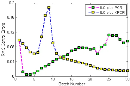
asR=0.01I . The performance of updated PCR model based ILC and that of updated KPCR model based ILC are shown in Fig. 3. It can be seen from Fig. 3 that, although the RMS errors of updated KPCR model based ILC are larger than those of updated PCR model based ILC in the previous 12 batch runs, the error gradually

Figure 1. Comparison of RMS control errors using fixed PCR model based ILC and fixed KPCR model based ILC under normal condition

TABLE III.

THE END-POINT QUALITIES IN THE 30TH BATCH RUN OF ALL CASES USING PCR MODEL BASED ILC AND KPCR MODEL BASED ILC

y30(tf)

with disturbances

without disturbances Case1 Case2

PCR-ILC KPCR- ILC PCR-ILC KPCR- ILC PCR-ILC KPCR- ILC

x1(tf) 0.7907 0.7923 0.8053 0.7991 0.8162 0.8099

x2(tf) 0.9981 0.9974 1.0005 1.0007 1.0576 1.0089

x3(tf) 0.9923 0.9915 1.0032 0.9984 1.0747 1.0073

Figure 2. Comparison of RMS control errors using updated PCR model based ILC and updated KPCR model based ILC in disturbance case 1

decreases after the 9th batch run as batch number increases afterwards. In contrast, although the RMS error of updated PCR model based ILC decreases in the first four batch runs, it increases gradually when batch number increases afterwards. It indicates that updated KPCR model based ILC can adapt the process variations in the case while updated PCR model based ILC cannot. The results demonstrate that KPCR model can capture the batchwise changed dynamics more effectively than PCR model and leads to more adaptive performance control. Table 3 presents the control performances of the two ILC strategies in the 30th batch run of all simulated cases.

V.CONCLUSIONS

A batch-to-batch model-based iterative learning control strategy for the tracking control of the end point product quality of batch processes is proposed. To address the problem of nonlinearities in batch processes, a nonlinear model for end-point product quality prediction, linearized around the nominal batch trajectories, is identified from process operating data using KPCR technique. On the basis of the linearized KPCR model, an ILC law is obtained explicitly by calculating the optimal control profile. To address the problems of unknown disturbances and process variations, the KPCR model should be updated from batch to batch to capture the changed batch process dynamics. After each batch run, the latest data are added to the data set and the earliest data are removed from the data set to rebuild the model. Based on the updated model, an adaptive ILC is derived to overcome process variations or disturbances. The proposed technique is illustrated on a simulated batch polymerization process. The results demonstrate that the ILC using KPCR model can adapt process variations or disturbances better than the ILC using PCR model.

ACKNOWLEDGMENT

This work was supported by the Chinese 863 Program under Grant 2013AA013804 and the National Natural Science Foundation of China under Grant 61064004.

REFERENCES

[1] T. Clarke-Pringle, and J. F. MacGregor, “Nonlinear adaptive temperature control of multi-product, semi-batch polymerization reactors,” Computers & Chemical Engineering, vol. 21, pp.1395–1409, 1997.

[2] C. Gentric, P. Filiberto, M. A. Latifi, and J. P. Corriou, “Optimization and non-linear control of a batch emulsion polymerization reactor,” Chemical Engineering Journal, vol. 75, pp.31–46, 1999.

[3] W. Xie, S. Rohani, and A. Phoenix, “Extended kalman filter based nonlinear geometric control of a seeded batch cooling crystallizer,” The Canadian Journal of Chemical Engineering, vol. 80, pp.167–172, 2002.

[4] M. V. Lelann, M. Cabassud, and G. Casamatta, “Modeling, optimization and control of batch chemical reactors in fine chemical production,” Annual Reviews in Control, vol. 23, pp.25–34, 1999.

[5] J. Valappil, and C. Georgakis, “State estimation and nonlinear model predictive control of end-use properties in

batch reactors,” Proceedings of the American Control Conference, pp.999–1004, June 2001.

[6] N. M. Aziz, M. A. Hussain, and I. M. Mujtaba, “Performance of different types of controllers in tracking optimal temperature profiles in batch reactors,” Computers and Chemical Engineering, vol. 24, pp.1069–1075, 2000. [7] K. Y. Rani, and S. C. Patwardhan, “Data-driven model

based control of a multi-product semi-batch polymerization reactor,” Chemical Engineering Research and Design, vol. 85, pp.1397–1406, 2007.

[8] Suguru Arimoto, Sadao Kawamura, and Fumio Miyazaki, “Bettering operation of robots by learning,” Journal of Robotic systems, vol. 1, pp.123–140, 1984.

[9] K. L. Moore, Iterative Learning Control for Deterministic System, Springer, New York, 1993.

[10]K.S. Lee, I. S. Chin, H. J. Lee, and Jay H. Lee, “Model predictive control technique combined with iterative learning for batch processes,” AIChE Journal, vol. 45, pp.2175–2187, 1999.

[11]J. H. Lee, K. S. Lee, and W. C. Kim, “Model-based iterative learning control with a quadratic criterion for time-varying linear systems,” Automatica, vol. 36, pp.41– 659, 2000.

[12]K. S. Lee, and J. H. Lee, “Iterative learning control-based batch process control technique for integrated control of end product properties and transient profiles of process variables,” Journal of Process Control, vol. 13, pp.607– 621, 2003.

[13]Z. H. Xiong, and J. Zhang, “A batch-to-batch iterative optimal control strategy based on recurrent neural network models,” Journal of Process Control, vol. 15, pp.11–21, 2005.

[14]J. Zhang, “Batch-to-batch optimal control of a batch polymerisation process based on stacked neural network models,” Chemical Engineering Science, vol. 63, pp.1273– 1281, 2008.

[15]Z. H. Xiong, Y. X. Xu, J. Zhang, and J. Dong, “Batch-to-batch control of fed-“Batch-to-batch processes using control-affine feedforward neural network,” Neural Computing & Applications, vol. 17, pp.425–432, 2008.

[16]J. F. Cerrillo, and J. F. MacGregor, “Iterative learning control for final batch product quality using partial least squares models,” Industrial and Engineering Chemistry Research, vol. 44, pp. 9146–9155, 2005.

[17]J. H. Chen, and K. C. Lin, “Batch-to-batch iterative learning control and within-batch on-line control for end-point qualities using MPLS-based dEWMA,” Chemical Engineering Science, vol. 63, pp.977–990, 2008.

[18]B. Schölkopf, A. Smola, and K. B. Müller, “Nonlinear component analysis as a kernel eigenvalue problem,”

Neural Computation, vol. 10, pp.1299–1319, 1998. [19]R. Rosipal, and L. J. Trejo, “Kernel partial least squares

regression in reproducing kernel hilbert space,” Journal of Machine Learning Research, vol. 2, pp.97–123, 2001. [20]J. M. Lee, C. K. Yoo, and I. B. Lee, “Fault detection of

batch processes using multiway kernel principal component analysis,” Computers and Chemical Engineering, vol. 28, pp.1837–1847, 2004.

[21]Y. W. Zhang, Y. P. Fan, and P .C. Zhang, “Combining kernel partial least-squares modeling and iterative learning control for the batch-to-batch optimization of constrained nonlinear processes,” Industrial Engineering and Chemical Research, vol. 49, pp.7470–7477, 2010.

Journal of Chemical Engineering, vol. 17, pp.427–436, 2009.

[23]R. Rosipal, M. Girolami, L. J. Trejo, and A. Cichocki, “Kernel PCA for feature extraction and de-noising in nonlinear regression,” Neural Computing & Applications, vol. 10, pp.231–243, 2001.

Ganping Li was born in Nanchang City, China on June 4, 1972. He received the B.S. degree in electrical engineering from Tianjin University, Tianjin, China, in 1995, the M.S. degree in chemical mechanical engineering from Nanchang University, Nanchang, China, in 2002, and the Ph.D. degree in electrical engineering from Shanghai Jiao Tong University, Shanghai, China, in 2007.