Study on Partial Least-Squares Regression Model of Simulating Freezing Depth Based on Particle Swarm Optimization

Study on Partial Least-Squares Regression Model

of Simulating Freezing Depth Based on Particle

Swarm Optimization

Tianxiao Li

School of Water Conservancy & Civil Engineering / Northeast Agricultural University, Harbin, China

Email: [email protected]

Qiang Fu ※

, Fanxiang Meng, Zilong Wang and Xiaowei Wang

School of Water Conservancy & Civil Engineering / Northeast Agricultural University, Harbin, China

Email: [email protected], [email protected]

Abstract

—

In order to improve fitting and forecasting precision and solve the problem that some data with less sensitivity lead to low simulation precision of partial least-squares regression (PLS for short) model, the new method of simulating freezing depth is presented according to ground temperature of different depths, air temperatures, surface temperatures and the like. Firstly, the PLS model, which is built by virtue of the ideas of principal component analysis and canonical correlation analysis, can be adopted to solve the multi-correlation among each factor effectively by extracting principal components. And the interpretation ability of each principal component to freezing depth can be obtained by assistant analysis. Meanwhile, particle swarm optimization algorithm (PSO) is adopted to optimize partial regression coefficient, and then the PLS model based on PSO can be built. Compared with traditional PLS model, the optimized model has more reliability and stability, and higher precision.

Index Terms—freezing depth, particle swarm optimization, simulation, partial least-squares regression, principle component

I. INTRODUCTION

Frozen soil is a phenomenon that soil containing water is freezing when the temperature drops to 0 _℃ or below 0_℃. Frozen soil is a kind of extremely sensitive soil medium to temperature change [1]. Therefore, soil temperature has an important effect on frozen soil, and temperature change can affect regional distribution of soil

and freezing depth. The area of frozen soil, including permafrost and seasonal frost, accounts for about 20% of the earth’s land area [2]. Frozen soil processes in cold regions play an important role in climate change and weather forecasting [3-5]. Seasonal freeze-thaw layer is above annual change layer of temperature, near to surface, which is more sensitive to temperature change. It is generally known that frozen soil is an important part of soil situation and soil freezing depth is closely related to agriculture, architecture, railway design, road and bridge design and so on. The impact of temperature change on frozen soil not only affects those industries above, but also environment [6-7]. Therefore, it is of great significance to study the change of freezing depth.

The traditional regression method filters the pre-decided factors and solves coefficients, but if there is a severe relevance among the pre-decided factors, the analysis results will be bad or even invalid. However, Partial Least-Squares Regression (PLS) can solve this problem better [8-10]. Because the PLS model has better simulation to some sensitivity data and the less simulation to some insensitivity data, the accuracy of partial regression analysis modeling is limited to some degree [11].

Particle Swarm Optimization (PSO), which is an evolutionary computation technology based on the swarm intelligence, is proposed by Kennedy and Eberhart in 1995 [12]. The basic idea is a swarm intelligence and parallel searching algorithm through cooperation and competition among particles. PSO has many advantages such as the faster convergence rate, satisfying results in multi-dimensional function space optimization, dynamic target optimization, so it has been widely applied in many fields [13]. In that case, PSO is adopted to optimize partial regression coefficient, and then the PSO-PLS model is built on the basis of making PLS model. At the same time, this model is applied to forecast freezing depth.

First author: Li Tianxiao(1984-), male, Xinxiang City in Henan Province, master, mainly engaged in agriculture water and soil resources utilization and optimization and system analysis

II. THE MODELING IDEAS OF PLS MODEL

A. A brief introduction of PLS model

Partial least squares (PLS) regression is a new statistical method for modeling quantitative relationships between two blocks of variables Y and X, developed by

H. Wold [14-16] in 1983 and it is used as alternative to other different methods: least squares regression and principal components regression [17-20]. With this linear regression model, each dependent (response) variable Yi in the block Y can be obtained from a linear combination of the p independent (predictor) variables Xi in the X block according to equation [21]:

ε

β

β

β

β

+ + + + +

= p p

i X X X

Y 0 1 1 2 2 " (1)

Wherein, β_i are the regression coefficients and are determined with the calibration set and ε is the error.

B. working target

When there is only one response variable (there is only one response variable in this paper, namely, freezing depth), PLS model is short for PLS1 model [22-25].Suppose

y

∈

R

n , response variable set

] , , ,

[x1 x2 xp

X = " ,

x

_j

∈

R

n , if we want to adopt least squares regression to build the regression model of

y

to

x

₁

,

x

₂

,

"

,

x

_p , the p-estimator of regression

coefficients is

B

₌

₍

X

T

X

₎

−1

X

T

Y

_{. When all response}

variables are completely correlative,

(

X

T

X

)

_{is a}

noninvertible matrix. So the regression coefficient

B

can not be obtained by this formula. When all response variables are more correlative, the value of

X

T

X

is

close to zero, then the inverse matrix of

X

T

X

has serious rounding error. Therefore, the least squares regression is invalid, parameter estimation can be destroyed and the robustness of model can be lost. If we adopt these data to model, the regression coefficient of

j

x

is always hard to explain, even appears opposite sign in real life.

This problem can be well solved by PLS model. Compared with traditional multivariate statistical methods, there are some prominent characteristics:

1) Under the condition of existing serious multi-correlation among response variables, PLS can regress.

2) PLS can be applied to regress the place where the sample number is less than the number of response variable.

3) The last model of PLS consists of all response variables

4) PLS model is easier to distinguish information and noise of system

5) Each regression coefficient is easier to be interpreted in the PLS model

C. Modeling method

Given one dependent variable y, p independent variables {x1, x2… xp} and n observing sample points, the table between X = [x1, x2,…,xp]n×p and Y = [y]n×1 can be formed. PLS model extracts the components t1 and u1 from X and Y respectively. In order to meet the need of regression analysis, the following requirements must be satisfied [22-25]:

1) t1 and u1 ought to carry as much varied information as possible.

2) The correlation between t1 and u1 must reach the maximum.

PLS model does the regression of X on t1 and Y on t1 after extracting the first component t1 and u1, and the algorithm ends if the accuracy of regression equation meets the demand. Otherwise, the residual information of

X and Y, which is explained by t1, is done the second round of extracting the components and repeated until the precision reaches the satisfactory accuracy. If t1, t2… tm are extracted at last, PLS model will do the regression of

Y on t1, t2… tm, and then the regression equation of y about x1, x2… xp is represented. In the process of extracting components, the cross effectiveness is adopted to fix on the number of components.

D The cross effectiveness discriminant

Usually, PLS regression equation does not need to use all components (

t

₁

,

t

₂

,

"

,

t

_A) to model and it adopts the interception way to select the previous

m

components (

m

<

A

,

A

=

rank

(

X

)

). The model with better prediction performance can be obtained by only using these

m

components (

t

₁

,

t

₂

,

"

,

t

_A). If the follow-up components can not offer more meaningful information for interpreting

F

₀ , the way of adopting more components will only undermine the understanding of the statistical trends and leading to wrong forecasting results [22-25].

In the process of building partial least squares regression model, how many components should be selected on earth? Whether it has remarkable improvement for the model’s forecasting function after adding one component. Then we adopt the cross effectiveness to discriminate: all samples set after removing some sample points can be seen as a sample and a regression equation can be fitted using

h

components and then the eliminating sample points can be put into the previous fitting equation, the fitting value

) ( i h

y

₋

of

y

_i in the sample point

i

can be obtained. Each sample point repeats the above calculation. Define the sum of prediction error squares of

y

_i as

press

_h , namely,

∑

= −

−

=

n

t

i h i

h

y

y

press

1

2 )

(

)

In addition, regression equations containing h

components are fitted by all sample points. If

∧

hi

y

is the predictive value of the ith sample point, then sum of error square of

y

_i can be defined as

ss

_h, namely,

∑

=

−

=

n

i i hi

h

y

y

ss

1

2

)

(

(3)

Generally speaking,

press

_h

>

ss

_h, and

ss

_h

<

ss

_h−1, but which is bigger,

ss

_h−1 or

press

_h?

ss

_h−1 is fitting error of equation with (

h

−

1

) components fitted by all sample points.

press

_h added a component b, but containing disturbance error of sample point. If

press

_h is smaller than

ss

_h−1, to some extent, then it is considered that forecasting precision can be obviously improved by

adding a component

t

_h. Therefore, the smaller 1 − h h

ss

press

is, the better it is, namely,

2 1

95

.

0

≤

− h h

ss

press

(4)

The cross effectiveness discriminant can also be defined as, 1 2

₁

−

−

=

h h h

ss

press

Q

(5)

If

Q

_h2≥ (1-0.9025)=0.0975, it indicates that the quality of model can be improved by adding component, otherwise not.

III. THEFUNDAMENTALOFPSO

Suppose in D-dimension target searching space, there is a community including N particles. The position of the

ith particle is represented a D-dimension vector X = (xi1, xi2… xid); the historical optimal position of the ith particle is represented Pi = (Pi1, Pi2… Pid). The optimal position searched by all particles from now on is notated as Pg = (Pg1, Pg2 … Pgi). The speed of the ith particle is also a D -dimension vector V = (vi1, vi2… vid), it determines the displacement of particles in the searching space. Therefore, PSO is an arithmetic based on iteration idea. PSO adjusts their corresponding positions according to the following formula (6) and (7) [26-29]:

(

)

(

k

)

gd k gd k id k id k id k id

x

p

r

c

x

p

r

c

V

V

−

+

−

+

=

+ 2 2 1 1 1

⎩

⎨

⎧

>

=

−

<

−

=

max max max max

v

v

v

v

v

v

v

v

id id id id (6) 1 1 +

+

₌

₊

k

id k id k

id

x

v

x

(7)

Wherein,

1

≤

i

≤

N

,

1

≤

d

≤

D

, k is the iteration times(k≥0); The acceleration constants c1 and c2 are nonnegative number; r1 and r2 are the random number between 0 and 1; vmax is a constant, which limits the max speed value. The speed of the particle is bigger when vmax is bigger, which is suitable for global search. But it is possible to fly across the optimal solution. If vmax is smaller the particle may be in a specific area to search carefully. The arithmetic ends when the max iteration time reaches the iterative limiting value or the global optimal solution is steady.

IV. THEMODELINGSTEPSOFPLSBASEDONPSO Partial regression coefficients, which are the decision variables of the PSO optimization equation, are retained after building PLS model. And then the objective function on the decision variables can be obtained. The neighboring area of partial regression coefficients is the definitional domain, it will be adjusted according to the computing result and the new partial regression coefficients can be obtained. Compared with the original PLS model, the algorithm will be ended until the optimization results are satisfied.

The main modeling steps are as follows:

1) According to the ideas of PLS modeling, the freezing depth forecasting model is established. And then the partial regression coefficients are regarded as the decision variables of PSO optimization equation;

2) Fix on constraints and fitness function. The constraints are the definitional domain of each decision variable. Defined the fitness function as follows:

∑

=

−

=

m i i i

ni

y

y

y

m

x

f

1

1

[(

)

/

]

1

)

(

min

(8)

∑

=

−

=

m i i i

di

y

y

y

n

x

f

1

2

[(

)

/

]

1

)

(

min

(9)

Wherein, min f1(x) is the minimum fitting relative error; min f2(x) is the minimum reserved inspection relative error; m is the sample size; n is the reserved inspection sample size; yni is the fitting value of freezing depth, mm; ydi is the reserved inspection value of freezing depth, mm; yi is the measured value of freezing depth, mm. In order to find the optimal results, (8) and (9) all need to reach minimum. Now the two fitness functions are to combine to form one function by the weight method [30], the last fitness function is as follows:

)

(

min

)

(

min

)

(

min

f

x

=

α

₁

f

₁

x

+

α

₂

f

₂

x

1 2 1+α =

α (10)

3) Fix on the process and control parameters of PSO, including the initialized swarm number N, the acceleration constants c1 and c2，the maximum flying speed limiting value vmax and the end iterating time k.

4) Optimization and solution build PSO-PLS model and print optimization results.

V. EXAMPLEANALYSIS

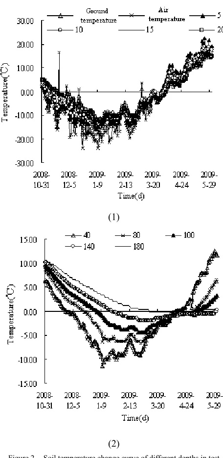
There are many factors affecting freezing depth of soil, but soil temperature is the most important one. In winter, the surface and soil temperature reduces gradually with the decreasing of air temperature. When soil temperature is lower than freezing temperature of soil, the soil begins to freeze. Therefore, the frozen-thaw process of soil is closely related to soil temperature.

A. Data source

Freezing depth measured data (y) (For convenience, freezing layer thickness is used here) is regarded as the dependent variable, some factors such as air temperature (x1), land surface temperature (x2), soil temperature of 5cm depth (x3), soil temperature of 10cm depth (x4) , soil temperature of 15cm depth (x5), soil temperature of 20cm depth (x6), soil temperature of 40cm depth (x7) , soil temperature of 80cm depth (x8) , soil temperature of 100cm depth (x9) , soil temperature of 140cm depth (x10), soil temperature of 180cm depth (x11), are selected as the independent variables. The stage data from Nov. 6, 2008 to Mar. 4, 2009 are used to build model, the data from Mar. 5, 2009 to Mar. 16, 2009 are used to inspect the accuracy of model.

According to experiment data, frozen-thaw curve and temperature change curve can be drawn as figure 1 and figure 2.

From these figures we can see that the frozen-thaw process of seasonal frozen soil can be divided into two stages, namely, unidirectional freezing stage and bidirectional melting stage. In addition, the temperature curve in whole test cycle all generate fluctuation throughout zero centigrade, causing phase transition of soil moisture and change of soil frozen-thaw process.

Figure 1. Soil frozen-thaw curve

(1)

(2)

Figure 2. Soil temperature change curve of different depths in test period

B. Multiple correlation diagnosis

With the variance inflation factor to diagnose each independent variable, multiple correlation among them exists is checked up. Variance inflation factor is named as

j VIF)

( [10, 22], the expression is as follows:

1 2₎ 1 ( )

(VIF _j = −R_j − (11)

Wherein, Rj2 are the multiple correlation coefficients taking xj as the dependent variable to other independent variables. The max (VIF)j in all xj is usually regarded as the important index of the multiple correlation. If

correlation coefficient and variance inflation factors of each xj are shown in Table I.

TABLE I.

MULTIPLE CORRELATION COEFFICIENT AND VARIANCE INFLATION FACTOR OF EACH INDEPENDENT VARIABLE

variables x1 x2 x3 x4 x5 x6

Rj2 0.786 0.970 0.309 0.999 0.999 0.996 (VIF)j 4.662 33.70 1.446 855.76 948.34 254.76 variables x7 x8 x9 x10 x11 /

Rj2 0.998 0.998 0.997 0.999 0.997 / (VIF)j 423.36 406.52 386.07 675.02 366.28 /

From Table I, we can know that the multiple correlation coefficients of x2, x4~x11 are all above 0.9, and the max (VIF)j =948.3377>10, that is to say, there is a serious multiple correlation among those independent variables.

C. Build PLS model

First, the series of the independent and dependent variable are normalized by matlab7.1 [31]. Second, the PLS theory is applied to extract three principal components. The cross effectiveness result is shown in Table II.

TABLE II.

THE CROSS EFFECTIVENESS RESULT

Principal component 1 2 3 4

Calculated value 0.7785 0.6507 0.3128 -0.8164

Critical value 0.0975 0.0975 0.0975 0.0975

From Table II, we can know that the calculated value is less than 0.0975 when extracting three principal components, namely, that extracting three principal components t1, t2, t3 meet the demands. And then do the linear regression of y on t1, t2, t3, the multiple correlation coefficient can be obtained R=0.9903，F=0，the PLS model is as follows:

4653 . 79 7887 15 3515 14

8103 11 7977 6 1009 0

4619 3 0573 3 1353 3

9009 2 1330 2 6320 0

11 10

9 8

7

6 5

4

3 2

1

+ −

−

− −

−

+ +

+

− +

− =

∧

x . x .

x . x . x .

x . x . x .

x . x . x . y

(12)

D. Precision analysis

The correlation coefficient square of above mentioned three principle components, x1 to x11 ，and dependent variable y are shown in Table III.

TABLE III.

THE CORRELATION COEFFICIENT OF PRINCIPLE COMPONENTS, DEPENDENT VARIABLE AND INDEPENDENT

VARIABLE

r2 _x

1 x2 x3 x4 x5 x6

t1 0.3563 0.4020 0.1155 0.7360 0.8269 0.9407

t2 0.4568 0.5324 0.2033 0.2283 0.1387 0.0148

t3 0.0181 0.0001 0.2975 0.0113 0.0167 0.0286

r2 _x

7 x8 x9 x10 x11 y

t1 0.9676 0.9513 0.9095 0.8948 0.8830 0.8190

t2 0.0002 0.0380 0.0804 0.0867 0.0930 0.1376

t3 0.0139 0.0005 0.0041 0.0097 0.0120 0.0185

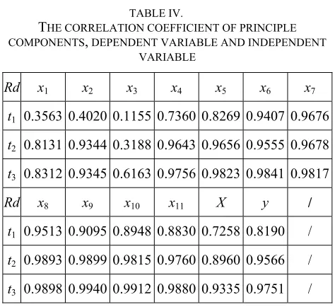
According to Table III, accumulated interpretation ability is calculated and shown as in Table IV. From the Table IV we can see that the accumulated interpretation ability of three components to independent is 93.35%，

and to dependent is 97.51%. From Table IV we can also see the independence of independent x3. Compared with all Rd, only x3 value is very small, just 0.6163, and the accumulated interpretation ability of three components to other independent variables and dependent variables are all up to 90%, except x1 is 83.12%.

TABLE IV.

THE CORRELATION COEFFICIENT OF PRINCIPLE COMPONENTS, DEPENDENT VARIABLE AND INDEPENDENT

VARIABLE

Rd x1 x2 x3 x4 x5 x6 x7

t1 0.3563 0.4020 0.1155 0.7360 0.8269 0.9407 0.9676

t2 0.8131 0.9344 0.3188 0.9643 0.9656 0.9555 0.9678

t3 0.8312 0.9345 0.6163 0.9756 0.9823 0.9841 0.9817

Rd x8 x9 x10 x11 X y /

t1 0.9513 0.9095 0.8948 0.8830 0.7258 0.8190 /

t2 0.9893 0.9899 0.9815 0.9760 0.8960 0.9566 /

t3 0.9898 0.9940 0.9912 0.9880 0.9335 0.9751 /

E. Build PSO-PLS model

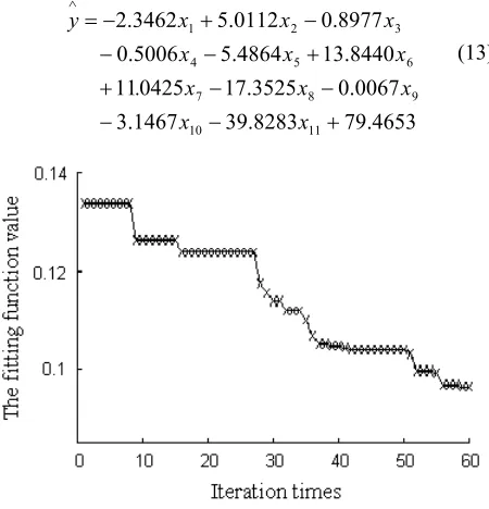
The regression coefficient is regarded as the original value of solving model. To prevent the algorithm precocious phenomena, the initial population number, the iteration time and the acceleration factors are tested and optimized repeatedly in the process of solving model. The final calculation results can be seen: the group size N＝

100, the iteration time k=60, the acceleration factors c1 =

60 times iteration when α1=0.81, α2 =0.19 . From figure 3, we can know that the fitness function tents to be stable. The final model after optimization is as follows:

4653 . 79 8283 . 39 1467 . 3

0067 . 0 3525 . 17 0425 11

8440 . 13 4864 . 5 5006 . 0

8977 . 0 0112 . 5 3462 . 2

11 10

9 8

7

6 5

4

3 2

1

+ −

−

− −

+

+ −

−

− +

− =

∧

x x

x x

x .

x x

x

x x

x y

(13)

Figure 3. Variation curve of fitness function value

F. Model comparative analysis

The optimization result goes back to (1) and (2), and the fitting relative error after optimization is 10.96%, the reserved inspection relative error is 3.97%. The model precision has greatly improved. In order to compare and analyze conveniently, the comparative analysis results of forecasting model are shown in Table V between in fitting stage and in forecasting stage.

TABLE V.

THE PREDICTION MODEL OF FREEZING DEPTH COMPARISON

Model type

Fitting stage relative error（%

）

absolute error（

cm）

Max Mean Max Mean PLS forecasting

model 936 26.54 24.21 6.08 PSOPLS

forecasting model 54.45 10.96 17.34 7.40

Model type

Forecasting stage relative error（%

）

absolute error（

cm）

Max Mean Max Mean PLS forecasting

model 15.14 13.00 22.94 19.59 PSOPLS

forecasting model 6.82 3.97 10.20 5.97

From Table V we know that the precision of PSO-PLS model has been improved greatly not only in fitting stage but also in forecasting stage, the average relative error in fitting stage is reduced by 58.7% and 69.4% in forecasting stage. Only in fitting stage the average absolute error of PLS model is better than the PSO-PLS model, which does not affect the overall prediction level. The fitting and forecasting curves are drawn respectively (figure 4 and figure 5). From figure 4 and figure 5 we also can see that the fluctuation amplitude of PSO-PLS model fitting curve is smaller than that of PLS model and the precision of PSO-PLS model is also higher. Thereby the model validity can be proved, and it can be used in the prediction of freezing layer thickness.

Figure 4. Contrast curve of freezing layer thickness in fitting stage

Figure 5. Freezing layer thickness contrast curve in prediction stage

VI. CONCLUSION

1) The variable can be processed by PLS model and the best explanation principal components can be extracted. On the one hand, the multiple correlations among variables can be solved; on the other hand, it can provide the foundation for optimizing the regression coefficient.

2) By assistant analysis, accumulative interpreting ability of freezing deep impact factor on freezing deep is derived. From the analysis results we can see that temperature has strongly independence, accounting for small proportion in the three principal components. According to actual observation, fluctuation of 5cm ground temperature changes greatly with temperature, which shows certain independence compared with other ground temperatures.

3) The PSO can be introduced into PLS modeling to optimize the regression coefficient. The multi-objective optimization thought is used to set up the fitness function and the multi-objective problem is solved by the trial method. This can not only improve the model fitting precision but also improve the prediction precision. The example shows that this method can provide a new approach for building freezing depth model. Therefore, it can expand the research idea of the freezing depth prediction.

ACKNOWLEDGMENT

Thanks to the support of Education Ministry of Specialized Research Fund for Doctoral Program “Study on the Complex Whole System Optimization Allocation Model of Regional Water and Soil resources based on CAS Theory” (NO.20092325110014), The Sub-Topic of National "Eleventh Five-Year" Scientific and Technological Support Plan “The Match Pattern of Regional Agricultural Soil and Water Resources and the Optimization of Crop Planting Structure” (No. 2009BADB3B02), Heilongjiang College Training Program for New Century Excellent Talents “Study on the Match Pattern and Sustainable Carrying Capacity of Agricultural Soil and Water Resource in Sanjiang Plain” (NO. 1155-NCET-004) and Harbin Special Fund for Technological Innovation “Study on the Soil and Thermal Coupling Movement Law and Numerical Simulation on the condition of Snow Cover” (NO. RC2010XK002013).

REFERENCES

[1] Guodong Cheng. Glaciology and Geocryology of China in the Past 40 Years: Progress and Prospect. Journal of Glaciolgy and Geocryology. vol. 20, no. 3, pp. 213-216, 1998

[2] Peixoto, J., and A. H. Oort Physics of Climate. American Institute of Physics, vol. 200 pp. 20-25 1992

[3] Mölders, N., and J. E. Walsh. Atmospheric response to soilfrost and snow in Alaska in March. Theor. Appl. Climatol., pp.77-115, 2004

[4] Poutou, E., G. Krinner, C. Genthon, and N. de Noblet-Ducoudré. Role of soil freezing in future boreal climate change. Climate Dyn., vol. 23, pp. 621-639, 1998

[5] Viterbo, P., A. Beljaars, J. F. Mahfouf, and J. Teixeira. The representation of soil moisture freezing and its impact on

the stable boundary layer. Quart. J. Roy. Meteor. Soc., vol. 125, pp. 2401-2426, 1999

[6] YANG Xiaoli, WANG Jing—song. The Change Characteristics of Maximum Frozen Son Depth of Seasonal Frozen Soil in Northwest China. Chinese Journal of Soil Science. vol. 39, no. 2, pp. 238-245, 2008

[7] XIA ZHANG, SHUFEN SUN, YONGKANG XUE. Development and Testing of a Frozen Soil Parameterization for Cold Region Studies. Journal of Hydrometeorology-special section. vol. 8, pp. 690-672, 2005

[8] Karen C. Weber · Káthia M. Honório · Aline T. Bruni · Adriano D. Andricopulo · Albérico B. F. da Silva. A partial least squares regression study with antioxidant flavonoid compounds. Struct Chem vol. 17, pp. 307–313, 2006 [9] Lourdes Cabezas · Miguel Angel González-Viňas · Cristina

Ballesteros · Pedro J. Martín-Alvarez. Application of Partial Least Squares regression to predict sensory attributes of artisanal and industrial Manchego cheeses. Eur Food Res Technol, vol. 222, pp. 223-228, 2006 [10] Fu Qiang, Wang Zhiliang and Liang Chuan, Modeling

Rice Evaporation with Partial Least-Squares Regression, Transactions of The Chinese Society of Agricultural Engineering, vol. 18, no. 6, pp. 9-12,2002

[11] Deng Nianwu, Chen Zheng and Ye Zerong, Modeling of Partial Least-Squared Regression and genetic algorithm in dam safety monitoring analysis, Dam & Safety, vol. 4, pp. 33-35, 2007

[12] Eberhart R C and Kennedy J, Swarm intelligence. San Francisco: Mornan Kaufmann Publishers, 2001

[13] Wei Xingqiong, Zhou Yongquan and Huang Huajuan. Adaptive particle swarm optimization algorithm based on cloud theory, Computer Engineering and Applications, vol. 45, no. 1, pp. 48-50, 76, 2009

[14] WoldH. In: Gani J (ed). Soft modeling by latents variables; the non-linear iterative partial least squares approach. New York, 1975

[15] I. Durán Merás · A. Espinosa Mansilla · F. Salinas López ·M. J. Rodríguez Gómez. Comparison of UV derivative-spectrophotometry and partial least-squares (PLS-1) calibration for determination of methotrexate and leucovorin in biological fluids. Anal Bioanal Chem, vol. 373 pp. 251–258, 2002

[16] Mateo Vargas · Fred A. van Eeuwijk Jose Crossa · Jean-Marcel Ribaut. Mapping QTLs and QTL × environment interaction for CIMMYT maize drought stress program using factorial regression and partial leastsquares methods. Theor Appl Genet, vol. 112, pp. 1009-1023, 2006

[17] Draper NR, Smith H. Applied regression analysis, 2nd edn. Wiley, New York, 1981

[18] Geladi P, Kowalski BR. Anal Chim Acta. vol. 185, pp. 1-17, 1986

[19] Sharaf MA, Illman DL, Kowalski BR. Chemometrics. Wiley, New York, 1986

[20] Martiın-Alvarez PJ. Quimiometria alimentaria. UAM (ed) Madrid, Spain, 2000

[21] Lourdes Cabezas. Miguel Angel González-Viňas. Cristina Ballesteros. Pedro J. Martín-Alvarez.Application of Partial Least Squares regression to predict sensory attributes of artisanal and industrial Manchego cheeses. Eur Food Res Technol. vol. 222, pp. 223-228, 2006

[22] Wang Huiwen. The application of Partial Least-Squares Regression Method. Beijing: National Defence Industry Press, 2000

Advances in Water Science, vol. 16, no. 6, pp. 822-825, 2005

[24] Fu Qiang and Liang Chuan. Water-Saving Irrigation System Modeling and Optimization Technique. Chengdu: Sichuan science and technology press, 2002

[25] Fu Qiang. The data processing method and its application in agriculture. Beijing: Science Press, 2006

[26] Yin Guoer, Zhang Zhanyu and Zhang Guohua. Multi-objective controlled drainage model based on particle swarm optimized algorithm. Transactions of The Chinese Society of Agricultural Engineering, vol. 25, no. 3, pp. 6-9, 2009

[27] Chen Dachun and Ma Yingjie. Optimized algorithm for estimating parameters by solving Van Genuchten equation based on stochastic particle swarm optimization. Transactions of The Chinese Society of Agricultural Engineering, vol. 22, no. 12, pp. 82-85, 2006

[28] Li Zhi and Zheng Xiao. Application of Improved Particle Swarm Algorithm in Optimization Design of Agricultural Engineering. Transactions of the Chinese Society of Agricultural Engineering, vol. 20, no. 3, pp. 15-18, 2004 [29] Zhang Libiao, Zhou Chunguang and Ma Ming. Solutions

of Multi-Objective Optimization Problems Based on Particle Swarm Optimization. Journal of Computer Research and Development, vol. 41, no. 7, pp. 1286-1291, 2004

[30] Xu Shuqin. Study on Water Resources Sustainable Utilization Planning Theory and Application of Irrigation Area. Northeastern Agriculture University, 2008

[31] Zhang Zhiyong. Proficient MATLAB6.5 version. Beijing: Beijing University of Aeronautics and Astronautics Press, 2003

Tianxiao Li, male, born in November 1984, master, mainly engaged in agriculture water and soil resources utilization and optimization and system analysis. The author obtained the bachelor degree of agriculture hydraulic project specialty in the Northeast Agricultural University in June 2007 and obtained the master degree of water and soil project in agriculture in the Northeast Agricultural University in June 2010. Recently, the author is a teacher in the Northeast Agricultural University. The number of participating in provincial projects is 2 and fulfilling actual production project is 6. More than 10 academic articles are published, in these articles, 3 articles are embodied by Engineering Index.

Qiang Fu, male, born in June 1973, professor, PhD supervisor, mainly engaged in agricultural soil and water resources system analysis, water-saving irrigation and agricultural systems engineering modeling and optimization technology. The number of presiding national and provincial projects is ten and the number of fulfilling actual production project is six. More than 150 academic articles and 6 monographs are published, in these articles, 50 articles are embodied by Engineering Index.