Initial and Boundary Value Problems Involving the Inhomogeneous Generalized Airy’s Equations

ISSN (e): 2250-3021, ISSN (p): 2278-8719

Vol. 07, Issue 03 (March. 2017), ||V1|| PP 11-27

Initial and Boundary Value Problems Involving the

Inhomogeneous Generalized Airy’s Equations

S.M. Alzahrani

1*

, I. Gadoura

2

, M.H. Hamdan

3+

1_{(Dept. of Mathematics and Statistics, University of New Brunswick, P.O. Box 5050, Saint John, New}

Brunswick, CANADA E2L 4L5

*On leave from University of Umm Al-Qura, Kingdom of Saudi Arabia.)

2_{(Dept. of Electrical and Computer Engineering, University of New Brunswick, P.O. Box 5050, Saint John, New}

Brunswick, CANADA E2L 4L5) 3

(Dept. of Mathematics and Statistics, University of New Brunswick, P.O. Box 5050, Saint John, New Brunswick, CANADA E2L 4L5)

Abstract: Initial and boundary value problems of the inhomogeneous Airy’s and generalized Airy’s differential equations are considered in this work. General solutions are expressed in terms of the Nield-Kuznetsov functions of the first and second kinds, and are computed when the forcing function is a constant or a variable function of the independent variable.

Keywords: GeneralizedAiry’s inhomogeneous equations, Nield-Kuznetsov functions.

________________________________________________________________________________________

I.

INTRODUCTION

In their pioneering work on flow through porous layers, as governed by Brinkman’s equation, Nield and Kuznetsov [1] introduced the concept of transition layer, defined here as a porous layer of variable permeability imbedded between two constant permeability porous layers, or one that is bounded by a constant permeability on one side and free-space on the other. They modelled the flow through the transition layer using Brinkman’s equation with variable permeability using a permeability function that ingeniously reduced the governing equation to an inhomogeneous Airy’s differential equation with constant forcing function. Solution to the flow problem was then attained in terms of an integral function,Ni(x), they introduced and defined in terms of Airy’s functions of the first and second kind, and used asymptotic series representations of Airy’s functions of the first and second kind to evaluate the Ni(x)function.

The Ni(x)function was subsequently studied extensively by Hamdan and Kamel [2] who documented its properties and extended its introduction to the integral function Ki(x) that arises in the solution of the inhomogeneous Airy’s equation with variable forcing function. The functions Ni(x)and Ki(x) have since been recognized as the Nield-Kuznetsov functions. Representations of these functions in terms of both asymptotic and ascending series have been obtained by Alzahrani et al. [3, 4], who provided a comparison of the solutions to flow through the transition layer using both of these series representations.

Abu Zaytoon et al. [5] approached the problem of flow through transition layer by modelling its permeability using a function that reduced the governing Brinkman’s equation to the generalized inhomogeneous Airy’s differential equation, of index n, with constant forcing function, and recovered the solution obtained by Nield and Kuznetsov [1] by choosing n = 1. We point out here that the generalized homogeneous Airy’s differential equation has been extensively studied by Swanson and Headley [6]. In case of the generalized inhomogeneous Airy’s equation with constant forcing function, Abu Zaytoon et al. [5] expressed its general solution with the help of a generalized form of the Nield-Kuznetsov Ni(x)function,

(i) Ni(x)and Ki(x) are termed the Standard Nield-Kuznetsov functions of the first- and second-kind, respectively. They arise in the solution to the inhomogeneous Airy’s equation with constant and variable forcing functions, respectively.

(ii) N_n(x)and K_n(x) are termed the generalized Nield-Kuznetsov functions of the first- and second-kind, respectively. They arise in the solution to the inhomogeneous generalized Airy’s equation of index n with constant and variable forcing functions, respectively.

The importance of the Airy’s and generalized Airy’s equations, and the above functions, in the modelling and solution of flow through porous layers, and their potential applications to other problems in mathematical physics motivates the current work in which we provide computations and analysis of initial and boundary value problems involving the inhomogeneous Airy’s and generalized Airy’s equations. Problem statements and solutions are provided for both constant and variable forcing functions in order to study the effects of the forcing functions on the solutions obtained.

II.

PROBLEM

FORMULATION

Required to solve the generalized Airy’s inhomogeneous ordinary differential equation (ODE): )

(y f u y

u n  …(1) subject to the initial conditions (I.C.)

 

) 0 (

u and u(0)   …(2)

where  and  are known constants, or subject to the boundary conditions (B.C.)

1 1)

(a b

u  and u(a₂)  b₂ ...(3)

where a₁,a₂,b₁and b₂ are real numbers.

In equation (1), n is a positive integer, prime notation denotes ordinary differentiation with respect to the independent variable y, and f(y) is the forcing function.

General solution to equation (1) is given by, [7]:

) ( ) sin( 2 ) ( ) ( 2

1 K y

m m y B c y A c

un n n n n n

 

 

 …(4)

where 2 1   n

m ,

c

_1n,

c

_2n are arbitrary constants, A_n(y)and B_n(y)are the generalized Airy’s functions of

the first- and second-kind, respectively, [6], and K_n(y)is the generalized Nield-Kuznetsov function of the second-kind, defined by, [7]

] ) ( ) ( ) ( ) ( ) ( ) ( [ ) ( 0 0





     y n n y n n

n y A y F t B t dt B y F t A t dt

K …(5)

with first derivative given by

             

( ) ( )

_

( ) ( ) ( )

_

( ) ( ) 2 sin( ) ( )

0 0 y F m m dt t A t F y B dt t B t F y A y K y n n y n n n   …(6)

wherein F(y)  f(y). When n=1, equation (1) reduces to the well-known Airy’s ODE whose general solution is given by, [7]:

) ( ) ( ) ( ₂

1Ai y c Bi y Ki y

c

u    …(7)

where Ai(y) and Bi(y) are Airy’s functions of the first- and second-kind, c₁ and c₂ are arbitrary constants,

and Ki(y) is the standard Nield-Kuznetsov function of the second-kind defined by, [7]:

] ) ( ) ( ) ( ) ( ) ( ) ( [ ) ( 0 0





     y y dt t i A t F y Bi dt t i B t F y Ai y

Ki …(8)

with first derivative given by

             

( ) ( )

_

( ) ( ) ( )

_

( ) ( ) 1 ( )

0 0 y F dt t i A t F y i B dt t i B t F y i A y i K y y

 . …(9)

) ( ) sin( 2 ) ( ) ( ₂

1 N y

m m y B c y A c

u_{n n n n n n}

 

 

 …(10)

and ) ( ) ( ) ( ₂

1Ai y c Bi y Ni y

c

u    …(11)

whereN_n(y)is the generalized Nield-Kuznetsov function of the first kind and Ni(y) is the standard

Nield-Kuznetsov function of the first-kind defined, respectively, by, [7]:





  y n n y n n

n y A y B t dt B y A t dt

N 0 0 ) ( ) ( ) ( ) ( )

( …(12)

and





  y y dt t Ai y Bi dt t Bi y Ai y Ni 0 0 ) ( ) ( ) ( ) ( )

( . …(13)

First derivatives of N_n(y) and Ni(y)are given, respectively, by





     y n n y n n

n y A y B t dt B y A t dt

N 0 0 ) ( ) ( ) ( ) ( )

( …(14)





     y y dt t Ai y i B dt t Bi y i A y i N 0 0 ) ( ) ( ) ( ) ( )

( . …(15)

In order to obtain complete solutions to the initial and boundary value problems, general solutions (4) must satisfy condition (2) for initial value problem and condition (3) for boundary value problem. This leads to determination of the arbitrary constants appearing in (4). In what follows, the arbitrary constants are determined for cases of constant and variable forcing functions, for the initial and boundary value problems.

III.

SOLUTION

TO

THE

INITIAL

VALUE

PROBLEMS

(IVP)

Using initial condition (2) in the general solution (4) results in the following values for the arbitrary

constants

c

_1n and

c

_2n:

) 0 ( ) 0 ( ) 0 ( ) 0 ( ) 0 ( ) sin( 2 ) 0 ( ) 0 ( 1 n n n n n n n n B A B A K m m B B c                      …(16) ) 0 ( ) 0 ( ) 0 ( ) 0 ( ) 0 ( ) sin( 2 ) 0 ( ) 0 ( 2 n n n n n n n n B A B A K m m A A c                      

. …(17)

Upon substituting (16) and (17) in (4), solution to the IVP is completely determined.

When the forcing function is of the form f (y)   , where  is a specified constant,

c

1n and

c

2n take the following forms:

) 0 ( ) 0 ( ) 0 ( ) 0 ( ) 0 ( ) 0 ( 1 n n n n n n n B A B A B B c     

   …(18)

) 0 ( ) 0 ( ) 0 ( ) 0 ( ) 0 ( ) 0 ( 2 n n n n n n n B A B A A A c      

   . …(19)

Upon substituting (18) and (19) in (7), solution to the IVP is completely determined.

IV.

SOLUTION

TO

THE

BOUNDARY

VALUE

PROBLEMS

(BVP)

Using boundary condition (3) in the general solution (4) results in the following values for the arbitrary





) ( ) ( ) ( ) ( ) ( ) ( ) ( ) ( ) sin( 2 ) ( ) ( 1 2 2 1 1 2 2 1 1 2 2 1 1 a B a A a B a A a B a K a B a K m m a B b a B b c n n n n n n n n n n n        …(20)





) ( ) ( ) ( ) ( ) ( ) ( ) ( ) ( ) sin( 2 ) ( ) ( 1 2 2 1 1 2 2 1 1 2 2 1 2 a A a B a A a B a A a K a A a K m m a A b a A b c n n n n n n n n n n n       

. …(21)

Upon substituting (20) and (21) in (4), solution to the BVP is completely determined.

When the forcing function is f (y)   , where  is a specified constant,

c

1n and

c

2n take the following forms:





) ( ) ( ) ( ) ( ) ( ) ( ) ( ) ( ) sin( 2 ) ( ) ( 1 2 2 1 1 2 2 1 1 2 2 1 1 a B a A a B a A a B a N a B a N m m a B b a B b c n n n n n n n n n n n        …(22)





) ( ) ( ) ( ) ( ) ( ) ( ) ( ) ( ) sin( 2 ) ( ) ( 1 2 2 1 1 2 2 1 1 2 2 1 2 a A a B a A a B a A a N a A a N m m a A b a A b c n n n n n n n n n n n       

. …(23)

Upon substituting (22) and (23) in (7), solution to the BVP is completely determined.

V.

COMPUTATIONS

OF

SOLUTIONS

TO

IVP

AND

BVP

V.1. Series Expressions for the Generalized Functions

Determination of values of the arbitrary constants, appearing in the IVP and BVP, and the evaluation of their solutions at particular values of the independent variable, y, necessitates evaluations of the standard and generalized Nield-Kuznetsov functions at the given values of y.

At the outset, the following values of the Nield-Kuznetsov functions at y = 0 have been obtained from their definitions, equations (5), (6), (8), (9), and (12)-(15), and used in deriving expressions (16)-(23) of the arbitrary constants: 0 ) 0 ( ) 0 ( ) 0

(  _n  _n 

n N K

N ,K i(0) 1 F(0)



 

 ; K_n(0) 2 m sin( m )F(0)

  



 . …(24)

Computations of the Airy’s, Generalized Airy’s, the standard and generalized Nield-Kuznetsov functions and their derivatives at any value of the independent variable y, are discussed in what follows.

The generalized Airy’s functions have been shown to have the following power series expansions [6]: )

( )

( )

(y g ₁ y g ₂ y

A_n _{n n}  _{n n} …(25)

m y g y g y

B_n( )  [_{n n1}( ) _{n n2}( )]/ …(26)

) 1 ( / )

(m1 m m

n   



 …(27)

) ( / )

(mm m

n  

 …(28)





       j p n j j j n m p p y m y g 1 ) 2 ( 1 2 1 ) ( 1 )

( …(29)

] ) ( 1 [ ) ( 1 ) 2 ( 1 2

2





       j p n j j j n m p p y m y y

g . …(30)

Equations (25)-(30) can evaluated at y = 0 to generate the values below for Airy’s and generalized Airy’s functions and their first derivatives, where the values of Airy’s functions and first derivatives at y = 0 are obtained using n=1 and m=1/3, (cf. [2,5,7]):

) 3 / 2 ( ) 3 / 1 ( ) 0 ( 3 / 2   Ai ; ) 3 / 1 ( ) 3 / 1 ( ) 0 ( 3 / 1     A ; ) 3 / 2 ( ) 3 / 1 ( ) 0 ( 6 / 1   Bi ; ) 3 / 1 ( ) 3 ( ) 0 ( 6 / 1   

B …(31)

The generalized Airy’s functions, given in equations (25) and (26), above, have been used by Alzahrani et al. [3,7] to derive the following series expressions for the generalized Nield-Kuznetsov functions N_n(y) and

) (y

K_n :

         

_

_

y n n y n n n n

n g y g t dt g y g t dt

m y N 0 1 2 0 2

1( ) [ ( )] ( ) [ ( )]

2 )

(   …(33)

            

_

_

y n n y n n n n

n g y F t g t dt g y F t g t dt

m y K 0 1 2 0 2

1( ) [ ( ) ( )] ( ) [ ( ) ( )]

2 )

(   . …(34)





_



         j p m j j j n m p p y j m y g 1 / 1 2 1 1 2 1 ) ( 1 ) ( 2 …(35)





] ) ( 1 ) 1 ( 1 ) ( 1 / 2 1 2 2 2





        j p m j j j n m p p y m j m y

g …(36)











        j p m j j j y n m p p y m j m y dt t g 1 / 1 1 2 2 0 1 ) ( 1 ) / 1 ( 1 )] ( [ 2 …(37)





] ) ( 1 ) / 2 ( 1 2 )] ( [ 1 / 2 2 1 2 2 0 2 2







        j p m j j j y n m p p y m j m y dt t

g . …(38)

Equations (24)-(38) are used to compute the generalized Airy’s and generalized Nield-Kuznetsov functions appearing in the solutions to the IVP and BVP. Computations are illustrated in the following numerical experiment.

V.2. Numerical Experiment

For constant forcing function f (y)   1/ and f(y)  1/ , and for variable forcing

functions f (y)  y, f(y) y2 and f (y)  sin y , suppose it is desired to solve equation (1) subject to the initial conditions u(0)  2,u(0) 1 and subject to the boundary conditions u(0) 1,u(1) 2.Then,

using equations (24)-(38), the integral functions appearing in expressions (16)-(23) for the arbitrary constants. Solutions (4) and (7) to IVP, and (10) and (11) to BVP, are then evaluated and plotted over the interval

1

0  y  for various values of generalized Airy’s parameter n, as discussed in the next section.

VI.

RESULTS

AND

DISCUSSION

VI.1. Solution to Airy’s Equation with Initial Values

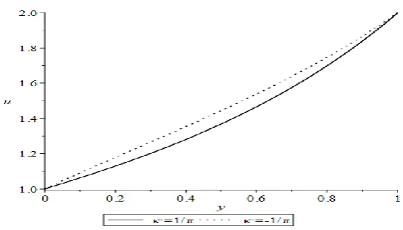
When n = 1, equation (1) is the well-known Airy’s differential equation. In this case, solutions (7) and (11) with initial conditions and with either constant or variable forcing functions result in the same values for the arbitrary constants, computed using expression (16)-(19): c₁ = 0.8848298434, c₂= 2.741563801. Solutions (7) and (11) are illustrated graphically in Fig. 1(a) and 1(b). For constant forcing functions, Fig. 1(a) illustrates solution (11) and shows an exponential increase in u(y) over the interval 0  y 1 for both f(y) 1/ , with a sharper increase when f(y)1/ . It is noted that the solutions obtained here using the discussed procedure is an alternative method to the solutions obtained for the same problem using Scorer functions, [2].

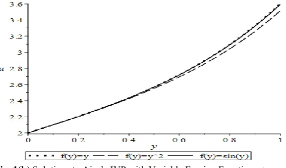
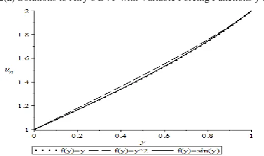
Fig. 1(b) illustrates solution (7) for the variable forcing functions f (y)  y ,

2

)

(y y

Fig. 1(a) Solutions to Airy’s IVP with Constant Forcing Function f (y)  1/

Fig. 1(b) Solutions to Airy’s IVP with Variable Forcing Function f(y)

VI.2. Solution to Airy’s Equation with Boundary Values

In this case, solutions (7) and (11) with boundary conditions and with either constant or variable forcing functions result in values for the arbitrary constants shown in Table 1. These have been computed using expressions (20)-(23).

Table 1. Values of arbitrary constants in the solution to BVP involving Airy’s equation.

) (y

f c₁ c₂

 /

1 0.2327830325 1.491812929

 / 1

 -0.3626315184 1.835575680 y 0.2417608772 1.486629567

2

y

0.08697595842 1.575994682

y

sin 0.2270128925 1.495144321

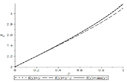
Solutions (7) and (11) are illustrated graphically in Fig. 2(a) and 2(b).For constant forcing functions, Fig. 2(a) illustrates solution (11) and shows the relative positions of the solution curves, and how the solutions increase, over the interval 0  y 1 for both f(y) 1/ . Fig. 2(b) illustrates solution (7) for the variable forcing functions f (y)  y , f(y) y2 and f(y)  sin y , and shows the relative positions and closeness of the solution curves for the functions tested. Again, solution curves are close to each other due to the closeness of the values of the functions over the interval 0  y 1. In both cases of constant or variable forcing

functions, solutions u(y) are higher for functions with lower values of y. In other words, over the interval

1

Fig. 2(a) Solutions to Airy’s BVP with Constant Forcing Function f (y)  1/

Fig. 2(b) Solutions to Airy’s BVP with Variable Forcing Function f(y)

VI.3. Solution to Generalized Airy’s Equation with Initial Values

In order to study the effects of increasing the generalized Airy parameter n on the solution to the inhomogeneous generalized Airy’s equation with initial conditions, solution to equation (1) is evaluated for n = 1, 2, 3, 4, 5 and 10. For the initial value problem with constant forcing function, expressions (18) and (19) for the arbitrary constants c_1n and c_2n are evaluated for various values of n and shown in Table 2. Solutions (10)

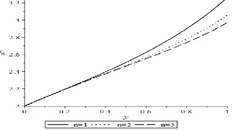
for u_n are evaluated and plotted for each of the constant functions f (y) 1/ in Fig. 3(a,b) and 4(a,b).

Fig. 3(a,b) illustrate u_n for f(y)1/ and the various values of n, while Fig. 4(a,b) illustrate u_n for 

/ 1 ) (y  

f and the various values of n. For visual clarity, the figures group the cases of n = 1,2,3 in one graph and n = 4,5,10 in another graph. All of these graphs show the relative positions of the solution curves with increasing n, and demonstrate the decrease in u_n with increasing n over the interval 0 y 1, with larger decrease as y increases. This pattern persists for both constant forcing functions considered.

Table 2. IVP Values of

c

_1n and

c

_2nfor different values of n and constant or variable f (y).



 1

)

(y   

f

1



n

_

n

c

₁ 0.88482984;

c

_2n



2.741563801

2



n

_

n

c

₁ 0.9023084857;



n

3



n

_

n

c

₁ 1.051988482;



n

c

₂ 3.303169579

4



n

_

n

c

₁ 1.272537560;



n

c

₂ 3.582773032

5



n

_

n

c

₁ 1.538574592;



n

c

₂ 3.849602302

10



n

_

n

c

₁ 3.224800671;



n

c

₂ 5.014277165

Fig. 3(a) Solutions to Generalized Airy’s IVP with Constant Forcing Function f(y) 1/ and n = 1, 2 and 3.

Fig. 3(b) Solutions to Generalized Airy’s IVP with Constant Forcing Function f(y)  1/ and n = 4, 5 and 10.

Fig. 4(b) Solutions to Generalized Airy’s IVP with Constant Forcing Function f(y)  1/ and n = 4, 5, 10. For the initial value problem with variable forcing functions, expressions (16) and (17) for the arbitrary constants c_1n and c_2n are evaluated for various values of n and shown in Table 2 for each of the variable

forcing functions considered. Solutions (4) for u_n are evaluated and plotted in Fig. 5(a,b), 6(a,b), 7(a,b) and

8(a,b).

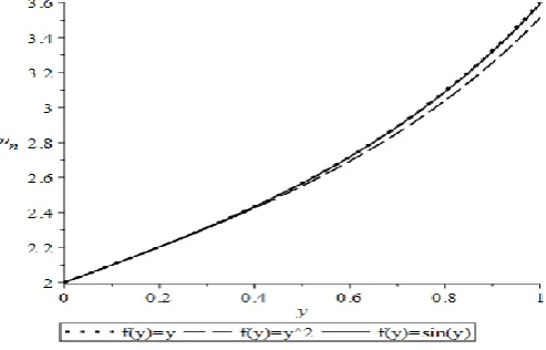
Fig. 5(a) illustrates u_n for n = 1 (namely, solution to Airy’s equation) and Fig. 5(b) illustrates u_n for n = 10, for various variable forcing functions. These figures demonstrate the similarity in qualitative behaviour of the solutions to Airy’s and generalized Airy’s equations for the different forcing functions tested.

Fig. 6(a,b), 7(a,b), 8(a,b) illustrate u_nfor f(y)  y, f(y)  y2 and f(y) sin y , respectively, and the various values of n. Again, for visual clarity, the figures group the cases of n = 1,2,3 in one graph and n = 4,5,10 in another graph. All of these graphs show the relative positions of the solution curves with increasing n, and demonstrate the decrease in u_n with increasing n over the interval 0  y 1, with larger decrease as y increases. This pattern persists for all forcing functions considered.

Fig. 5(b) Solutions to Generalized Airy’s IVP with Various Variable Forcing Functions f(y) and n = 10

Fig. 6(a) Solutions to Generalized Airy’s IVP with f(y) y and n = 1, 2, and 3

Fig. 7(a) Solutions to Generalized Airy’s IVP with

f

(

y

)



y

2 and n = 1, 2, and 3

Fig. 7(b) Solutions to Generalized Airy’s IVP with

f

(

y

)



y

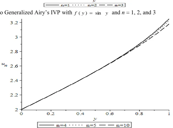
2 and n = 4, 5, and 10

Fig. 8(a) Solutions to Generalized Airy’s IVP with f (y)  sin y and n = 1, 2, and 3

Fig. 8(b) Solutions to Generalized Airy’s IVP with f (y)  sin y and n = 4, 5, and 10

VI.4. Solution to Generalized Airy’s Equation with Boundary Values

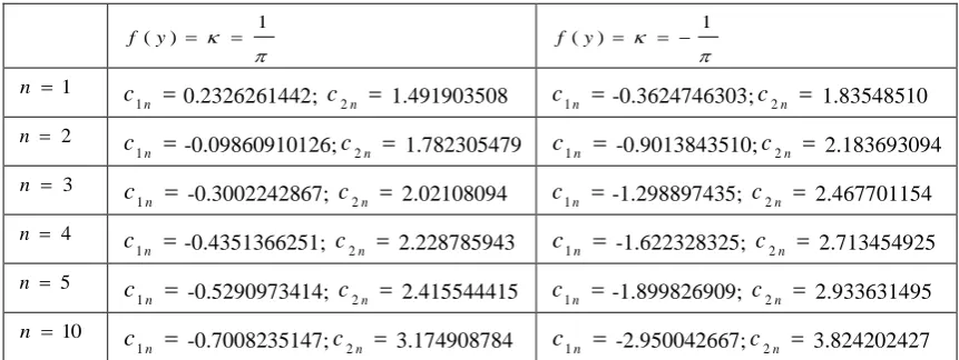
In order to study the effects of increasing the generalized Airy parameter n on the solution to the inhomogeneous generalized Airy’s equation with boundary conditions, solution to equation (1) is evaluated for n = 1, 2, 3, 4, 5 and 10. For the boundary value problem with constant forcing function, expressions (22) and (23) for the arbitrary constants c_1n and c_2n are evaluated for various values of n and shown in Table 3.

Solution (10) for u_n is evaluated and plotted for the constant functions f(y) 1/ . Fig. 9(a) illustrates

n

and f(y) 1/ , respectively, for various values of n. Again, for visual clarity, the figures group the cases of n = 1,2,3 in one graph and n = 4,5,10 in another graph. All of these graphs show the relative positions of the solution curves with increasing n, and demonstrate the increase in u_n with increasing n over the interval

1

0 y  . This pattern persists for both constant forcing functions considered.

Table 3. BVP values of

c

_1n and

c

_2nfor different values of n and constant f(y) .



 1

)

(y  

f



 1

)

(y   

f

1



n

_

n

c

₁ 0.2326261442;

c

_2n



1.491903508

c

_1n



-0.3624746303;

c

_2n



1.83548510

2



n

_

n

c

₁ -0.09860910126;

c

_2n



1.782305479

c

_1n



-0.9013843510;

c

_2n



2.183693094

3



n

_

n

c

₁ -0.3002242867;

c

_2n



2.02108094

c

_1n



-1.298897435;

c

_2n



2.467701154

4



n

_

n

c

₁ -0.4351366251;

c

_2n



2.228785943

c

_1n



-1.622328325;

c

_2n



2.713454925

5



n

_

n

c

₁ -0.5290973414;

c

_2n



2.415544415

c

_1n



-1.899826909;

c

_2n



2.933631495

10



n

_

n

c

₁ -0.7008235147;

c

_2n



3.174908784

c

_1n



-2.950042667;

c

_2n



3.824202427

Fig. 9(a) Solutions to Airy’s BVP with Constant Forcing Functions f (y)  1/

Fig. 10(a) Solutions to Generalized Airy’s BVP with Constant Forcing Function f (y)  1/ and n = 1, 2, and 3

Fig. 10(b) Solutions to Generalized Airy’s BVP with Constant Forcing Function f(y)  1/ and n = 4, 5, and 10

Fig. 11(a) Solutions to Generalized Airy’s BVP with Constant Forcing Function f(y)   1/ and n = 1, 2, and 3

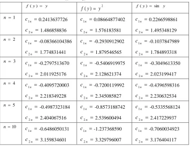
For the boundary value problem with variable forcing functions, expressions (20) and (21) for the arbitrary constants c_1n and c_2n are evaluated for various values of n and shown in Table 4 for each of the variable

forcing functions considered. Solutions (4) for u_n are evaluated and plotted in Fig. 12(a,b), 13(a,b), 14(a,b)

and 15(a,b).

Fig. 12(a) illustrates u_n for n = 1 (namely, solution to Airy’s equation) and Fig. 12(b) illustrates u_n for n = 10, for the three variable forcing functions considered. These figures demonstrate the similarity in qualitative behaviour of the solutions to Airy’s and generalized Airy’s equations for all forcing functions tested. When n =1, solution curves tend to be of parabolic shape with higher curvature than for the case of n = 10. This might indicate that for values of n higher than 10 the velocity profile tends to be a linearly increasing function.

Fig. 13(a,b), 14(a,b) and 15(a,b) illustrate u_nfor f(y)  y , f(y)  y2 and f(y)  sin y , respectively, and the various values of n. Again, for visual clarity, the figures group the cases of n = 1,2,3 in one graph and n = 4,5,10 in another graph. All of these graphs show the relative positions of the solution curves with increasing n, and demonstrate the increase in u_n with increasing n over the interval 0  y 1. This pattern persists for all forcing functions considered. In addition, with increasing n the solution curves tend to be closer together, thus indicating that n has a greater influence on the solution curves than the form of forcing function.

Table 4. BVP values of

c

_1n and

c

_2nfor different values of n and variable f (y).

y y

f ( )  2

)

(

y

y

f



f (y)  sin y

1



n

_

n

c

₁ 0.2413637726



n

c

₂ 1.486858836



n

c

₁ 0.08664877402



n

c

₂ 1.576183581



n

c

₁ 0.2266598861



n

c

₂ 1.495348129

2



n

_

n

c

₁ -0.08366104386



n

c

₂ 1.774831441



n

c

₁ -0.2930912902



n

c

₂ 1.879546565



n

c

₁ -0.1037847989



n

c

₂ 1.784893318

3



n

_

n

c

₁ -0.2797513670



n

c

₂ 2.011925176



n

c

₁ -0.5406919975



n

c

₂ 2.128621374



n

c

₁ -0.3049613350



n

c

₂ 2.023199417

4



n

_

n

c

₁ -0.4095720003



n

c

₂ 2.218349228



n

c

₁ -0.7200119992



n

c

₂ 2.345085827



n

c

₁ -0.4396598316



n

c

₂ 2.230632534

5



n

_

n

c

₁ -0.4987323184



n

c

₂ 2.404067516



n

c

₁ -0.8573188742



n

c

₂ 2.539600494



n

c

₁ -0.5335568124



n

c

₂ 2.417229937

10



n

_

n

c

₁ -0.6486050131



n

c

₂ 3.159834601



n

c

₁ -1.237368590



n

c

₂ 3.329796007



n

c

₁ -0.7060034923



n

Fig. 12(a) Solutions to Airy’s BVP with Variable Forcing Functions f(y)

Fig. 12(b) Solutions to Generalized Airy’s BVP with Variable Forcing Functions f (y)

Fig. 13(a) Solutions to Generalized Airy’s BVP with f(y) y, n = 1, 2, and 3

Fig. 14(a) Solutions to Generalized Airy’s BVP with

f

(

y

)



y

2, n = 1, 2, and 3

Fig. 14(b) Solutions to Generalized Airy’s BVP with

f

(

y

)



y

2, n = 4, 5, and 10

Fig. 15(b) Solutions to Generalized Airy’s BVP with f (y)  sin y , n = 4, 5, and 10

VII.

CONCLUSION

In this work we provided analysis and computations of the inhomogeneous generalized Airy’s ordinary differential equation with Airy’s index n, subject to initial and boundary conditions. The forcing functions chosen are either constant ( f(y)  1/k ) or variable (f(y) y; f(y) y2; f(y) sin y). The generalized Airy’s equation reduces to Airy’s equation when n = 1. General solutions to the inhomogeneous generalized Airy’s equation have been expressed and evaluated in terms of the generalized Nield-Kuznetsov functions of the first-kind (for constant forcing functions) and second-kinds (for variable forcing functions). When n = 1, the generalized Nield-Kuznetsov functions reduce to the standard Nield-Kuznetsov functions of the first and second kinds.

Solutions have evaluated using computational procedures based on series expressions for the generalized Airy’s functions and for the Nield-Kuznetsov functions. Arbitrary constants and the solutions are tabulated or graphed in this work, and support the following conclusions.

(a) Values of the arbitrary constants in the case of initial value problem are independent of the forcing function in Airy’s and generalized Airy’s equation, but are dependent on Airy’s index n.

(b) Values of the arbitrary constants in the case of boundary value problem depend on both the forcing function and Airy’s index.

(c) For both the initial and boundary value problems with constant or variable forcing functions, solutions are increasing over the interval 0 y 1, with exponentially varying solution curves for the initial value problem, regardless of the form of forcing function.

(d) With decreasing n, solution curves for the initial value problem experience sharper increase with increasing y.

(e) With increasing n, solution curves for the boundary value problem experience sharper increase with increasing y.

VIII.

REFERENCES

[1] D. A. Nield and A. V. Kuznetsov, The effect of a transition layer between a fluid and a porous medium: shear flow in a channel, Transport in Porous Media, 78, 2009, 477–487.

[2] M.H. Hamdan and M.T. Kamel, “On the Ni(x) integral function and its application to the Airy’s non-homogeneous equation, Applied Math.Comput., 217#17, 2011, 7349–7360.

[3] S.M. Alzahrani, I. Gadoura and M.H. Hamdan, Representations and Computation of the Nield- Kuznetsov Integral Function, ISOR Journal of Applied Physics,Vol. 8, Issue 3, Ver II, 2016, 55-67. [4] S.M. Alzahrani, I. Gadoura and M.H. Hamdan, Ascending series solution to Airy’s inhomogeneous

boundary value problem, Int. J. Open Problems Compt. Math., 9#1, 2016, 1-11.

[5] M.S. Abu Zaytoon, T.L. Alderson and M.H. Hamdan, Flow through a layered porous configuration with generalized variable permeability, Int. J. of Enhanced Research in Science, Technology & Engineering, Vol. 5 Issue 6, 2016, 1-21.

[6] C.A. Swanson and V. B. Headley, An extension of Airy's equation. SIAM J. Appl. Math. Vol. 15, 1967, 1400-1412.