ISSN (e): 2250-3021, ISSN (p): 2278-8719
Vol. 09, Issue 6 (June. 2019), ||S (IV) || PP 51-56
A Novel Method for Ensemble of Surrogates Based on Global and
Local Measures
Ying Luo
1, Jiajia Qiu
1, Jian Zhang
11Faculty of Civil Engineering and Mechanics, Jiangsu University, Xuefu Road 301, Zhenjiang, Jiangsu
Province, China, postal code: 212013 Corresponding Author: Jiang Zhang
Abstract:
Surrogate models are widely used in the community of engineering design and optimization to substitute computationally expensive simulations for efficient approximation of system behaviors. However, since the actual system behaviors are usually not known a priori, it is very challenging to select the most appropriate surrogate model for a specific application.To deal with this issue, an ensemble model that combines different surrogate models has been presented, and many efforts are devoted to the weight factor selection for the component surrogate models based on global measure and local measure respectively. In this paper, a novel ensemble of surrogate models is developed to take advantage of both global and local measures, and a unified strategy is conceived over the entire design space with proper tradeoff between these two measures. The effectiveness of the new ensemble model is tested on six mathematical benchmark examples with varying dimensionality. The results show that the proposed ensemble model has more desirable accuracy and robustness for a majority of test problems compared with the individual surrogate models and other ensemble models.Keywords:
Surrogate model, Metamodel, Ensemble, Global measure, Local measure.--- --- Date of Submission: 22-06-2019 Date of acceptance: 10-07-2019
---I.
INTRODUCTION
integration of global and local measures. No division of the design space is needed, and a unified strategy is devised over the entire domain with the trade-off between global and local error metrics.
II.
THE PROPOSED ENSEMBLE METHOD
The traditional technique of surrogate modeling is usually composed of constructing a number of different surrogates, selecting one with the best accuracy and discarding the rest candidates. Nevertheless, two major shortcomings exist. First, most of the resource spent on the construction of different surrogates is wasted. Second, the performances of different surrogates are dependent on the sample points, so there is no guarantee that the selected surrogate model will be accurate on a new data set. To overcome these drawbacks, an ensemble of surrogates rather than an individual one is proposed.An ensemble is a weighted average of several different surrogates. The resulting ensemble model is formulated as
𝑦 𝑒𝑛𝑠 𝑥 = 𝑤𝑖 𝑥
𝑁𝑠
𝑖=1
𝑦 𝑖 𝑥 (1)
where 𝑦 𝑒𝑛𝑠 𝑥 is the prediction value of the ensemble, Ns is the number of surrogates used, and wi is the weight factor for ith surrogate model 𝑦 𝑖 𝑥 . The weight factors are calculated with the following requirement
𝑤𝑖 𝑥
𝑁𝑠
𝑖=1
= 1 (2)
To maximize the prediction accuracy of an ensemble, the weight factors are selected such that the component surrogate with higher accuracy will occupy a larger proportion in the ensemble model and vice versa. According to the measures of evaluating the weight factors, existing ensemble modeling methods can be generally classified as global measures and local measures.
Goel et al. (2007) proposed an ensemble of surrogates based on global measures in which GMSE was used to select the weight factors from a heuristic formulation
𝑤𝑖 =
𝑤𝑖∗
𝑤𝑗∗ 𝑁𝑠
𝑗 =1
(3)
𝑤𝑖∗= 𝐸𝑖+ 𝛼𝐸 𝛽
𝐸 = 1
𝑁𝑠
𝐸𝑖
𝑁𝑠
𝑖=1
where 𝐸𝑖 is the GMSE of the ith surrogate model evaluated from
𝐸𝑖 =
1
𝑛 𝑦 𝑥𝑘 − 𝑦 𝑖
−𝑘 𝑥 𝑘
2 𝑛
𝑘=1
(4)
where n is the number of sample points, xk is the kth sampling point, y(xk) is the true response value at xk, and 𝑦 𝑖
−𝑘 𝑥
𝑘 is the corresponding prediction value of the ith surrogate model constructed using all except the kth sampling point. two parameters 𝛼 = 0.05 and 𝛽 =−1 were recommended by Goel et al. (2007).
As an alternative to using prediction variance, Acar (2010) proposed a spatial model in which the pointwise cross validation error was selected as the localerror measure.
𝑤𝑖 =
𝑤𝑖∗
𝑤𝑗∗ 𝑁𝑠
𝑗 =1
(5)
𝑤𝑖∗= 𝑊𝑖𝑘𝐼𝑘 𝑥
𝑛
𝑘=1
𝐼𝑘 𝑥 =
1 𝑑𝑘2 𝑥
𝑑𝑘 𝑥 = 𝑥 − 𝑥𝑘
al.(2007) and local measureproposed by Acar (2010) are integrated for ensemble modeling with a unified formulation over the entire design space. Taking advantage of multiple kinds of error metrics, the accuracy and robustness of the proposed unified ensemble of surrogates (UES) are enhanced with modeling efficiency nearly the same with other ensemble of surrogates.
To evaluate the accuracy of an ensemble surrogate, the commonly used error measures are cross-validation error, prediction variance and mean square error (or root mean square error) (Zhou et al. 2011). As no additional test (validation) points are required for error evaluation, the cross-validation error is selected to construct the UES model in this article. Cross-validation error, also known as leave-one-out cross-validation error, is the prediction error at each sample point while the surrogate model is built with the other (n−1) sample points. For ensemble modeling, the cross-validation error of the ith surrogate at the kth sample point is formulated as
𝑒𝑖𝑘 = 𝑦 𝑥𝑘 − 𝑦 𝑖
−𝑘 𝑥
𝑘 (6)
To have a fair comparison and to reduce the computational cost as well, the same error matrix is adopted to construct all ensemble surrogates. And the weight factors can be obtained as follows
ℒ𝐺 𝑒𝐶𝑉 ⇒ 𝑤𝐺
ℒ𝐿 𝑒𝐶𝑉 ⇒ 𝑤𝐿 (7)
where eCV denotes the error matrix computed from cross-validation error, ℒ𝐺 . and ℒ𝐿 . represent the strategies of calculating the weight factor by using global measure (wG, named global weight factor) and the weight factor by using local measure (wL, named local weight factor) respectively.
Global measures evaluate the weight factors of individual surrogates with an overall model accuracy from the entire error matrix. Local measures regard weight factors as the diversity indicator of component surrogates at different locations in the design space, so the weight factors at a prediction point are severely affected by the adjacent sample points. Therefore, local measures dominate in the evaluation of weight factors when the prediction point is near to the sample points, while global measures are more suitable for prediction points far from the sample points. To this end, a unifiedensemble of surrogates (UES) with global measure and local measure is proposed to define the weight factors for the entire design space as:
𝑤𝑖 =
𝑤𝑖∗
𝑤𝑗∗ 𝑁𝑠
𝑗 =1 (8)
𝑤𝑖∗= 𝑤𝑖𝐺𝜆 𝑥 + 𝑤𝑖𝐿 1 − 𝜆 𝑥
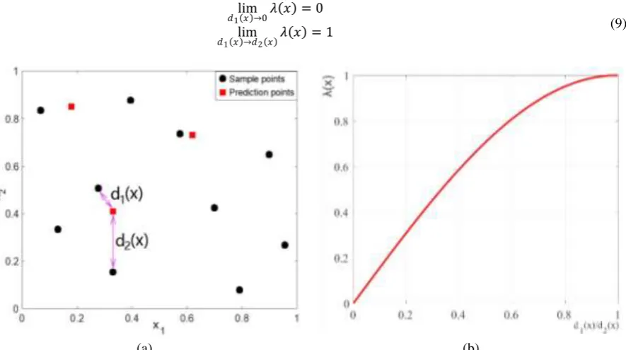
where 𝑤𝑖𝐺 and 𝑤𝑖𝐿are respectively global weight factor and local weight factor for the ith surrogate model. 𝜆 𝑥 is the coefficient of measure impact to control the influence regions of global and local measures on calculating the weight factors at the prediction point x.the coefficient 𝜆 𝑥 must satisfy the following conditions:`
lim
𝑑1 𝑥 →0𝜆 𝑥 = 0 (9)
lim
𝑑1 𝑥 →𝑑2 𝑥
𝜆 𝑥 = 1
(a) (b)
where, as shown in Figure.1(a), d1(x) is the distance between the prediction point x and its nearest sample point, d2(x) is the distance between x and its second-nearest sample point. In this study, the Sine function, as shown in Figure.1(b), were selected as candidate coefficient functions.
𝜆 𝑥 = sin 𝜋
2
𝑑1 𝑥
𝑑2 𝑥
(10)
III.
EXAMPLE PROBLEMS
Six well-known mathematical benchmark problems varying from 2-D to 12-D are chosen to test the characteristics of the UES models: (1) Branin-Hoo function (2-D); (2) and (3) are Hartman functions (3-D and 6-D, denoted as Hartman-3 and Hartman-6 respectively); (4) Dette and Pepelyshev function (8-D); (5) Griewank function (8-D) and (6) Dixon-Price function (12-D). Detailed information on these functions can be found in Table1.
Table 1:Summary of benchmark problems
Function Dimension Formulation Definition
domain
(1) 2 𝑓 𝑥 = 𝑥2−5.1𝑥1
2
4𝜋2 +
5𝑥1
𝜋 − 6
2
+ 10 1 − 1
8𝜋 cos 𝑥1+ 10
[-5,10; 0,15]D
(2) 3 𝑓 𝑥 = − 𝑐𝑖𝑒𝑥𝑝 − 𝑎𝑖𝑗 𝑥𝑗− 𝑝𝑖𝑗
2 3
𝑖=1 4
𝑖=1
[0,1]D
(3) 6 𝑓 𝑥 = − 𝑐𝑖𝑒𝑥𝑝 − 𝑎𝑖𝑗 𝑥𝑗− 𝑝𝑖𝑗
2 6
𝑖=1 4
𝑖=1
[0,1]D
(4) 8
𝑓 𝑥 = 4 𝑥1− 2 + 8𝑥2− 8𝑥22 + 3 − 4𝑥22 2
+16 𝑥3+ 1 2𝑥3− 1 2+ 𝑖𝑙𝑛 1 + 𝑥𝑖
8
𝑖=4
[0,1]D
(5) 8 𝑓 𝑥 = 1
4000 𝑥𝑖
2 8
𝑖=1
− cos 𝑥𝑖
𝑖
8
𝑖=1
+ 1 [0,1]D
(6) 12 𝑓 𝑥 = 𝑥1− 1 2+ 𝑖 2𝑥𝑖2− 𝑥𝑖−1 2
12
𝑖=2
[0,10]D
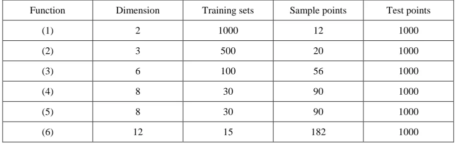
For the design of experiments (DOE) of all benchmark problems, Latin hypercube sampling (LHS) technique is employed to select the locations of the training and test points. Table 2 presents the summary of training sets, sample points and test points for all benchmark problems.
Table 2:Summary of the training and test point sets used in the benchmark problems
Function Dimension Training sets Sample points Test points
(1) 2 1000 12 1000
(2) 3 500 20 1000
(3) 6 100 56 1000
(4) 8 30 90 1000
(5) 8 30 90 1000
(6) 12 15 182 1000
𝑅2= 1 − 𝑦𝑖− 𝑦 𝑖
2 𝑁𝑡𝑒𝑠𝑡
𝑖=1
𝑦𝑖− 𝑦 2
𝑁𝑡𝑒𝑠𝑡
𝑖=1
(11)
𝑁𝑀𝐴𝐸 = 𝑚𝑎𝑥 𝑦𝑖− 𝑦 𝑖
1 𝑁𝑡𝑒𝑠𝑡
𝑦𝑖 − 𝑦 𝑖 2
𝑁𝑡𝑒𝑠𝑡
𝑖=1
Where 𝑁𝑡𝑒𝑠𝑡 is the number of test points, std denotes the standard deviation of samples and mean is the mean value, 𝑦𝑖is the true value calculated by the benchmark functions, 𝑦 𝑖is the corresponding prediction value of the surrogate model and 𝑦 is the meanvalue of 𝑦𝑖.The value of 𝑅2 iscloser to 1 and the value of 𝑁𝑀𝐴𝐸 iscloser to 0, the closer the predictionsurrogate model is to the real benchmark function.
The accuracy and robustness of the UES models are compared with two existing ensemble models, namely: (i) the heuristic algorithm developed by Goel et al. (2007) (labeled by EG), (ii) the spatial model proposed by Acar (2010) (labeled by SP). Three representative surrogate models, polynomial response surface (PRS), radial basis functions (RBF), Kriging (KRG), are used as the component surrogates for all ensemble models and are also compared with the ensemble models. The results are shown in the following figure.
Figure 2:𝑅2of ensemble and individual surrogate models
Figure 3:NMAE of ensemble and individual surrogate models
IV.
CONCLUSION
International organization of Scientific Research
56 | Page
individual surrogate models and selecting the appropriate baseline models to be included for the UES ensemble model.REFERENCES
[1]. Myers RH, Montgomery DC (2002) Response surface methodology: process and product optimization using designed experiments. Wiley, New York
[2]. Fang HB, Horstemeyer MF (2006) Global response approximation with radial basis functions. Engineering Optimization 38(4):407–424.
[3]. Liu GR, Zhang J, Li H, Lam KY, Kee BBT (2006) Radial point interpolation based finite difference method for mechanics problems. International Journal for Numerical Methods in Engineering 68(7):728– 754
[4]. Martin JD, Simpson TW (2005) Use of kriging models to approximate deterministic computer models. AIAA Journal 43(4):853–863.
[5]. Clarke SM, Griebsch JH, Simpson TW (2005) Analysis of support vector regression for approximation of complex engineering analyses. Journal of Mechanical Design 127(6):1077–1087.
[6]. Goel T, Haftka RT, Wei S, Queipo NV (2007) Ensemble of surrogates. Structural and Multidisciplinary Optimization 33(3):199–216.
[7]. Acar E, Rais-Rohani M (2009) Ensemble of metamodels with optimized weight factors. Structural and Multidisciplinary Optimization 37(3):279–294.
[8]. Acar E (2010) Various approaches for constructing an ensemble of metamodels using local measures. Structural and Multidisciplinary Optimization 42(6):879–896.
[9]. Zhang J, Chowdhury S, Messac A (2012) An adaptive hybrid surrogate model. Structural and Multidisciplinary Optimization 46(2):223–238.
[10]. Liu HT, Xu SL, Wang XF, Meng JG, Yang SH (2016) Optimal weighted pointwise ensemble of radial basis functions with different basis functions. AIAA Journal 54(10):3117– 3133.
[11]. Chen LM, Qiu HB, Jiang C, Cai XW, Gao L (2018) Ensemble of surrogates with hybrid method using global and local measures for engineering design. Structural and Multidisciplinary Optimization 57(4):1711–1729.