(IJC)
ISSN 2307-4523 (Print & Online) © Global Society of Scientific Research and Researchers
http://ijcjournal.org/
Complementary Graph Coloring
Mohamed Al-Ibrahim
a*, Naser Al-Ibrahim
b, Yousef Rafique
c, Omar Al-Sumait
daComputing Department, KILAW, Doha, Kuwait
b,c,dComputer Engineering Department, Kuwait University, Khaldyia, Kuwait
aEmail: [email protected]
bEmail: [email protected]
cEmail: [email protected]
dEmail: [email protected]
Abstract
The objective of the Graph Coloring problem is to color vertices of a graph in such a way that no two vertices
that share an edge are assigned the same color. Aircraft Scheduling, Frequency Assignment, register allocation
are all real life applications that can be solved using graph coloring. Graph Coloring is a well-known
NP-complete problem to the academia in computer science and mathematics. In this paper we use the concept of
complementary graphs to come up with a new heuristic for graph coloring. Our results are compared with an
exact algorithm and other heuristic algorithms to evaluate our algorithm’s performance.
Keywords: Graph Coloring; Complementary Graphs; Chromatic Number.
1.Introduction
Graph Coloring is one of the most common optimization problems in the field of computer science and
mathematics. There have been many approaches to solve this problem using approximations and heuristics.
There are various real life applications of graph coloring, which include allocating radio frequencies in cellular
networks, exam scheduling, air traffic scheduling and register allocation. These systems can be modelled as
graphs, where we have a set of limited number of resources (colors) assigned to a set of variables (nodes) under
certain incompatibility constrains (edges).
1.1.Definitions
• A Graph G (V,E) is a set of vertices V (nodes) which are connected through edges E (links)
• A Connected Graph is a graph where each node can reach every other node
• A Directed Graph is a graph where the relationship between two vertices is implied one way. That is,
there exists a relation between vertex a→b, but a relation between b→a does not exist. This is referred
to as an ordered pair of edges
• An Undirected Graph is a graph where each edge is not associated with any order, where the edge (a,b)
is identical to the edge (b,a)
• Adjacent nodes are nodes connected through an edge, therefore if an edge exists between vertex A and
vertex B then A is adjacent to B
• The Chromatic Number of graph G is the minimum number of colors required to properly color a graph and is represented by χ(G)
• Degree of a vertex A is the number of edges connected to that vertex
• A Clique of size k is a completely connected sub-graph of graph G that contains k vertices
• Saturation degree of a given vertex is number of differently colored neighbors connected to it
1.2.Problem Statement
To color a graph G we must assign each vertex in the graph a specific color. To properly color this graph we
have to ensure that no two adjacent vertices are assigned the same color. The challenge in such a problem is
finding the chromatic number required to color this graph. Such a problem is known to be NP-Complete because
there is no efficient algorithm that can solve this problem in polynomial time. The proof of NP-Completeness is
done by reducing the problem to another well known NP-Complete problem [4].
In this work we propose a new greedy algorithm that is based on complementary graphs and evaluate its
performance. The rest of this paper is organized as follows; Section 2 illustrates the related work that others
have done in this area. Section 3 contains our detailed approach along with the pseudo code of our algorithm.
Finally, Section 4 contains evaluation and comparison of our algorithm along with other approaches in the
literature.
2.Related Work
Most optimal graph coloring solutions in the literature are based on greedy algorithms, where finding locally
optimal solutions would lead to a globally optimal solution. These greedy algorithms depend on ordering the
nodes in a certain way, ordering of the nodes significantly affects the overall performance. The work done by
Welsh & Powell in [8] is based on this greedy concept, where they model the graph as a set of points and
construct an incompatibility matrix M, where 𝑀𝑀𝑖𝑖𝑖𝑖 = 1 if there exist an adjacent node in an undirected graph.
They achieve graph coloring by bounding the chromatic number χ(G)≤ d+1 to the highest degree. This is done
by first sorting the vertices in descending order based on the magnitude of their degrees and picking a color for
will then repeat the previous procedure recursively at the next highest degree number and picking a new color
until all nodes are colored.
Other work proposed by Brelaz in [1] was the DSTAUR branch and bound algorithm which was based on
Welch’s work. DSTAUR uses dynamic sequential coloring where it employs the greedy approach to pick the
vertex with the highest saturation degree. Similar to Welsh, it starts by assigning color 1 to the vertex with the
highest degree. Then it orders vertices by descending saturation degrees. More commonly, this can be
represented as the maximum clique, where the clique size determines the lower bound for the chromatic
number. Each vertex is a assigned a set of allowable colors. It repeatedly selects the vertex with the highest
saturation degree and assigns it the smallest valid color from the set of allowable colors. However, in the event
of a tie of saturation degrees, the algorithm selects the vertex with the highest number of uncolored neighbors.
Further ties are handled lexicographically. This approach of dynamically picking the highest saturation degree at
each iteration aims to reduce the chromatic number. For every partial coloring at each step a new sub problem is
created to branch into forming a search tree, therefore the branch and bound approach. Reaching a leaf node in
the search tree determines the current upper bound for the chromatic number. Finally, the algorithm terminates
when the lower bound = upper bound.
The previous algorithm determines the exact chromatic number, but has a very high complexity. Such problems
are classified as NP-Complete as it requires exhaustive trials of all valid coloring combinations to determine the
best coloring possible [2]. Lawler was the first to tackle this in [3] by introducing a polynomial time O(2.445n)
algorithm that uses dynamic programming to quickly determine the exact chromatic number for a given graph.
He achieves this by bounding the number of maximal independent sets (MIS) to 3n/3.
To reduce the number of sub-problems generated by the branch and bound algorithm, Sewell in [6] proposed a
new saturation degree tie breaking strategy that selects the vertex with the highest number of common allowable
colors that it shares with its neighbors, rather than the highest degree of uncolored neighbors. As a further
improvement to the original algorithm PASS algorithm was proposed in [5], which imposes further restrictions
limiting the number of sub-problems. Similar to Sewell, in case of a tie it selects the vertex with maximum
common available colors shared with its neighbors, but this time the only qualifying vertices are those with the
highest chromatic numbers, while the rest are eliminated.
The authors in [7] introduced a new graph coloring algorithm based on breadth first search (BFS). The
algorithm first creates an array of colors, where the size is equal to the number of nodes in the graph. The array
is initialized with a single color c. The algorithm starts by selecting a pivot node that it chooses either randomly
or heuristically. This pivot node is considered the root of the BFS search tree, traversing through all the
outgoing edges marking them with the same color. It then repeats the previous step, until all the graph is colored
and creates multiple disjoint sets. While traversing through the outgoing edges a condition must be satisfied; if
color of visited node is smaller than the pivot’s color, it is assigned the pivot’s color. Subsequently, the
algorithm traverses through the incoming edges starting at the pivot and it removes vertices with incompatible
3.Our Approach
Figure 1: Original Graph
Any graph G can be represented as a V x V matrix where V is the number of vertices in the graph such that each
element in the matrix 𝐸𝐸𝑖𝑖𝑖𝑖 is an edge from vertex i to vertex j. Each edge in the matrix has the value of 0 or 1,
where 0 means no edge exists between the vertices and 1 means an edge exists between the vertices. (See Figure
1)
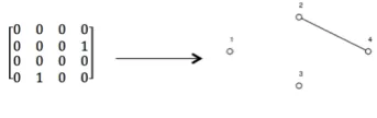
Figure 2: Complementary Graph
Let G = (V, E) be a graph, the complement of G denoted as G' has the same vertices of G such that if and only if
an edge e exists between 𝑉𝑉𝑖𝑖 & 𝑉𝑉𝑖𝑖 in G, 𝑉𝑉𝑖𝑖 & 𝑉𝑉𝑖𝑖are disconnected in G' and if 𝑉𝑉𝑖𝑖 & 𝑉𝑉𝑖𝑖 are disconnected in G, they
have to be connected in G'. Given a matrix as a graph G we can easily find G' by flipping the 0’s and 1’s and
ignoring the diagonal. (See Figure 2)
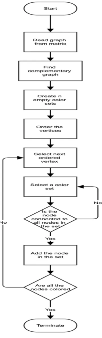
We approached this problem by coloring the complement of a graph G given in the form of n x n matrix. To
color G’ first we have to create n empty color sets. Vertices of G’ are ordered based on a specific order scheme
discussed in the following section. Vertices are traversed in order and are added to a color set by satisfying the
following condition:
𝑉𝑉𝑖𝑖 → ∃ 𝐸𝐸𝑖𝑖𝑖𝑖 ∀ 𝑉𝑉𝑖𝑖 ∈ 𝐶𝐶𝐶𝐶𝐶𝐶𝐶𝐶𝐶𝐶𝐶𝐶𝐶𝐶𝐶𝐶𝐶𝐶 (1)
This condition says that for a vertex i to be added to a color set; it must contain an edge to every node in that set,
else it checks for compatibility with the next set. After traversing all the vertices and adding them to our color
sets, we remove all the empty color sets. The number of color sets remaining denotes our chromatic number.
(See Figure 3)
From our previous graph, since we have 4 nodes we will create 4 empty color sets. We order the vertices from
the complementary graph G’ in a specific order, say highest degree to lowest degree. These vertices are initially
Table 1: Step 1
Ordered Vertices Empty Sets
4, 2, 1, 3 Color Set 1 = {} Color Set 2 = {}
If the degree of a vertex is tied with another vertex we can randomly select a vertex. In our example we will
choose vertex 4 and 1 before vertex 2 and 3 respectively. According to Figure 3 we select the next ordered
vertex, which is vertex 4 from the set of uncolored vertices. We start to check the compatibility of vertex 4 with
the color sets using Equation 1. Vertex 4 is compatible with the first color set, therefore it is added to that set.
Color set 1 will contain vertex 4 and the rest of the color sets will remain empty.
Table 2: Step 2
Ordered Vertices Empty Sets
4, 2, 1, 3 Color Set 1 = {4} Color Set 2 = {}
Vertex 4 is removed from the set of uncolored vertices and the next ordered vertex is selected. The next vertex
selected from the set is 2. We check if vertex 2 is compatible with color set 1. Vertex 2 is compatible, therefore
we vertex 2 is added to color set 1. Color set 1 will contain vertex 4 and 2 and the rest of the color sets will
remain empty.
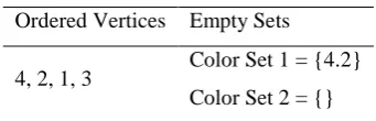
Table 3: Step 3
Ordered Vertices Empty Sets
4, 2, 1, 3 Color Set 1 = {4.2} Color Set 2 = {}
After inserting all the nodes in the color sets vertex 4 & 2 are in the same set, vertex 1 & 3 in separate sets. By
removing the empty sets our chromatic number will be the number of used sets, that is 3.
The main data structure used to implement complementary graph coloring is an array where the input to the
algorithm is a graph represented by an adjacency matrix and the out- put is a colored graph along with its
chromatic number. Two arrays are maintained, one for the ordered nodes set and the other for the color set.
Upon ordering the nodes the resulted ordered nodes are maintained in the ordered nodes set. When coloring any
node, the location of the node is added to the color set array. Since the graph is represented by an adjacency
color set array is a special array, where each cell represents a color and contains a linked list containing the
nodes associated with that color.
Table 4: Step 4
Ordered Vertices Empty Sets
4, 2, 1, 3 Color Set 1 = {4.2} Color Set 2 = {1}
The order of the nodes is an important issue, since order can significantly affect the outcomes of an algorithm.
In our approach four different orderings were used; highest degree to lowest (order 1), lowest degree to highest
(order 2), random order (order 3) and ordering based on connected and disconnected graphs (order 4).
Table 5: Step 5
Ordered Vertices Empty Sets
4, 2, 1, 3
Color Set 1 = {4.2}
Color Set 2 = {1}
Color Set 3 = {3}
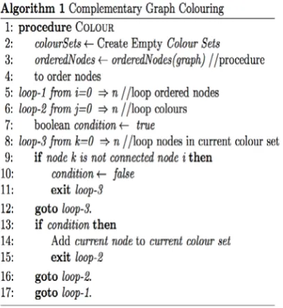
Figure 4 shows a pseudo-code for our algorithm. In figure 5 we compare the different types of order schemes
based on the yielded chromatic number. Ordering the nodes from lowest degree to highest degree (order 2) in
the complementary graph outperformed in contrast with the other ordering schemes. Based on these results
ordering scheme 2 was chosen in our approach.
Figure 5: Ordering Comparison
4.Evaluation
The algorithms were implemented in Java environment and each of them evaluated identical graph input. A
different graph is generated randomly using a randomizer, producing unique graphs with varying number of
vertices ranging between predetermined bounds for every run. In every run each algorithm evaluates the graph
and computes the chromatic number for a valid coloring. The generated graph can range from a weakly
connected graph to a strongly connected graph taking into account all types of graphs. We ran the program for
200 runs generating random graphs with nodes ranging between 1000-5000. After running the program for 200
runs we calculated the average chromatic number for each algorithm as shown in fig 6.
Table 6: Running Time Complexities
Approaches Big O Complexity
Complementary Graph O(𝑐𝑐 ∗ 𝑛𝑛3)
Welsh & Powell O(𝑐𝑐 ∗ 𝑛𝑛3)
BFS Approach O(𝑐𝑐 ∗ 𝑛𝑛3)
Exact DSATUR Exponential
Complexity
We observed from the results obtained that the complementary graph coloring yielded a chromatic number
roughly identical to Welsh. DASTUR is an exact approach where it gives us a solution within the close vicinity
of the optimal solution.
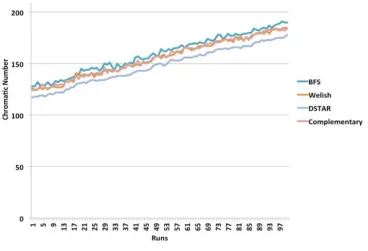
Figure 7: Chromatic Number Comparison
Figure 7 clearly demonstrates the relationship between the chromatic number and the number of nodes. As the
number of nodes increases, so does the chromatic number required to color the graph properly. We noticed that
BFS contributed to the highest chromatic number, while our algorithm and Welsh performed closely similarly.
DSTAUR however, out- performed all the other algorithms in terms of chromatic number due to its exact
coloring characteristic.
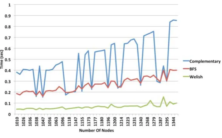
As illustrated in fig 8, DSATUR was eliminated for a fair comparison as it was producing exponential times
results in magnitudes of seconds, while the others algorithms were running in polynomial time in magnitudes of
milliseconds. The running time increases as the number of nodes increases, but we noticed a fluctuation which
was caused due to the nature of the random graph generated at each run. Heavily connected graphs consumed
higher times, while weakly connected graphs exhibited minimal times. Welsh clearly outperforms BFS and
complementary graph coloring algorithms by a factor of 𝑛𝑛
log 𝑛𝑛. The difference between our algorithm and Welsh
is the sorting technique used. Welsh uses a heap sort method to order his nodes, while our approach used the
classic bubble sort method to implement its ordering there- fore introducing a gap. As n grows the dominating
factor of both algorithms will be O(𝑛𝑛3) therefore this gap can be neglected. It can also be observed that BFS’s
performance is similar to our approach and Welsh due to the fact of coloring each disconnected graph in O(𝑛𝑛2)
time yields a worst case analysis of O(c * 𝑛𝑛3). We can conclude that as the number of nodes in the graph grows,
Figure 8
5.Conclusion
It can be concluded from our study of different colouring algorithms, that Welsh-Powell has demonstrated to be
the ideal algorithm in terms of run time and chromatic number. However, as shown from our results DSATUR
produces the closest to optimal chromatic numbers, but at an extremely high run time cost as compared to other
approaches mak- ing impractical. On the contrary, our approach colours the graph in a reasonable manner,
producing chromatic numbers similar to Welsh and a running time complexity identical to BFS.
Future work involves experimenting our algorithm with dif- ferent data structures such as heaps that is used by
Welsh, with the intention of reducing the overall running time com- plexity. Since both of our algorithms have
O(n2) running time complexity, by using a different data structure we be- lieve that we could achieve better
running than Welsh.
References
[1] D. Br ́elaz. New methods to color the vertices of a graph. Communications of the ACM, 22(4):251–
256, 1979.
[2] M. R. Garey and D. S. Johnson. Computers and intractibility: a guide to the theory of np-completeness.
WH Freeman and Company, New York, 18:41, 1979.
[3] M. R. Garey, D. S. Johnson, and L. Stockmeyer. Some simplified np-complete problems. In
Proceedings of the sixth annual ACM symposium on Theory of computing, pages 47–63. ACM, 1974.
[4] E. L. Lawler. A note on the complexity of the chromatic number problem. Information Processing
Letters, 5(3):66–67, 1976.
[5] P. San Segundo. A new dsatur-based algorithm for exact vertex coloring. Computers & Operations
Research, 39(7):1724–1733, 2012.
[6] E. Sewell. An improved algorithm for exact graph coloring. DIMACS series in discrete mathematics
and theoretical computer science, 26:359–373, 1996.
[7] G. M. Slota, S. Rajamanickam, and K. Madduri. Bfs and coloring-based parallel algorithms for strongly
connected components and related problems. In IEEE International Parallel and Distributed Processing
Symposium, 2014.
[8] D. J. Welsh and M. B. Powell. An upper bound for the chromatic number of a graph and its application