Extracting Structured Data From Raw Recipe Text (Natural Language Processing)

(1)

Extracting Structured Data From Raw Recipe Text

(Natural Language Processing)

Peter Zhang

Department of Computer Science Stanford University [email protected]

1 Introduction

When people cook today, they often refer to one of millions of recipes on the internet, which may contain non-standardized ingredients and ingredient quantities. The goal of this project is to train a model to extract structured data from the ingredient list of a recipe. This structured data is useful for a variety of purposes: generating an aggregated grocery list, computing nutrition information, and generating meal plans given various nutritional goals and other preferences. These tools may be especially relevant given recent events - many people are at home and cooking more than they used to due to COVID-19.

Concretely, we wish to take a ingredient description (1 line of an ingredient list) from a recipe as input, and output structured data about that ingredient: mapping the ingredient to a database of standard ingredients, identifying the quantity of the ingredient used, and capturing any descriptions of the way the ingredient was prepared or comments about the ingredient (see Figure1).

Figure 1: Example of input and desired output. One approach to this problem is to break the task into two pieces:

1. Semantic labeling: Tag each word in the ingredient text with its role (quantity, unit, ingredi-ent, prep, comment).

2. Mapping: Map all ingredient words to a standard ingredient from our database; map all unit words to a standard unit from our database, convert unit and quantity to a weight.

This project will focus on the first piece of this task, with the second piece left for future work.

2 Related work

The New York Times published a post describing their approach to this semantic labeling task. They used a linear-chain CRF with hand-picked feature functions to label ingredient phrases with the roles of each component word (1), and later released their code and dataset (2).

(2)

There is also a body of work by Korpusik and Glass that addresses a similar but more difficult problem: the extraction of structured data from meal descriptions. For the similar semantic labeling sub-task of this problem, they have tried several approaches, ranging from early work similar to the New York Times approach (CRF with hand-picked feature functions) (3) to more modern techniques like RNNs, CNNs, and fine-tuning BERT for their problem space (4).

Finally, there are some commercial products that appear to provide this functionality, but the approach they take to solving this problem is opaque (e.g.Paprika,Whisk,Zestful,Spoonacular,Edamam).

3 Dataset

The primary dataset I used is the one provided in theingredient-phrase-tagger github reporeleased by the New York Times (2).

This dataset consists of 179,207 raw ingredient phrases from the New York Times recipe database as of 2015, along with text columns giving the associated "name" (ingredient name), "qty" (quantity), "unit", "comment" and "range_end" (end of range of quantities) of each phrase.

After running this data through a tokenizer and tagger provided in the repo,1_{the dataset consists of} 1,102,763 tokens, with a tag distribution shown in Table11.

NAME UNIT QTY COMMENT RANGE_END OTHER

Count 327,465 120,650 150,438 352,542 1,864 149,804

Table 1: Tag distribution in NYT dataset.

I segmented this dataset into DEV and TEST datasets, each with 5,000 randomly selected sample sentences, and put the remaining 169,207 samples in the TRAIN dataset.

I also built a web tool to manually tag ingredient phrases (see details in AppendixA), and tagged an additional 3,000 examples by hand, 2,000 to be used as additional TRAIN examples, and 1,000 to be used as DEV examples. These examples came from a wider variety of online recipes (rather than only NYT cooking recipes), which better reflects the real-world distribution of recipes the model will be used on, and the accuracy of the labels is significantly higher than the NYT dataset.

4 Methodology

In an attempt to improve on the baseline model performance of83.7%tag-level accuracy achieved by the NYT (1) (2) (see AppendixBfor details on running the baseline), I built a series of models using Tensorflow and Keras (5) (6) with the following structure:

1. Embedding LayerA trainable embedding layer (tf.keras.layers.Embedding). 2. Recurrent Layers Various recurrent layers (tf.keras.layers.SimpleRNN,

tf.keras.layers.GRU, tf.keras.layers.LSTM, and bidirectional versions of all three), stacked 1, 2 or 3 layers deep.

3. Dense LayerA dense output layer with 11 units representing each of the possible tags.23

1

The tokenizer applies various specific tokenization rules, like joining whole and fractional number compo-nents and splitting certain weight abbreviations (e.g. 100g => 100 grams). The tagger uses heuristics to select the best tag for each token based on what is included in the "name", "qty", "unit", "comment" and "range_end" text columns. For full details, see (2).

2

This layer had a linear activation (and thus outputted logits) but a Softmax layer could be applied afterwards to get probabilities.

3

I used a BIO tagging strategy (so NAME, UNIT, QTY and COMMENT tags had B and I variants) similar to the baseline model, which is why there are 11 possible tags rather than the 6 mentioned earlier. B represents the beginning of a tagged phrase and I represents the interior of a tagged phrase; this allows us to identify two separate ingredient names in the same ingredient line of a recipe (e.g. salt (B-NAME) and (OTHER) black (B-NAME) pepper (I-NAME)), as the second ingredient name will start with a B-NAME tag as opposed to an I-NAME tag.

(3)

All models in this paper were trained using an Adam optimizer with the default hyperparam-eters using a batch size of 128, and with a standard categorical cross-entropy loss function (tf.losses.SparseCategoricalCrossentropy).

I iterated on this high-level model structure by performing an architecture search on the type of recurrent layer to use, and then tuning various hyperparameters, including the number of recurrent layers, the number of units per recurrent and embedding layer, and dropout regularization rates.

5 Experiments and Discussion

After experiencing some initial issues related to improper dataset shuffling (see AppendixE), I ran a series of experiments based on the methodology described above. All experiments were evaluated using word-level accuracy on the DEV set, but I also tracked sentence-level accuracy (did the model tag all words in an example correctly) as well.

5.1 NN Architecture Search

First, I did a basic architecture search, trying out a 64-unit simple RNN, GRU, and LSTM for the recurrent layer of my model, as well as bi-directional variants of all three, stacked on top of a 64-unit embedding layer. The bidirectional variants all outperformed the unidirectional variants, and the GRU and LSTM variants led the group in terms of word-level accuracy on both the TRAIN and DEV sets, but the differences were not very large across all options, with all TRAIN performance ranging

from83.6−86.1%accuracy and DEV performance ranging from80.4−81.6%accuracy. The full

results of these experiments can be seen in Table5in AppendixC.1.

The similar performance of GRUs and LSTMs vs. a simple RNN on this task was mildly surprising, but can likely be explained by the fact that most recipe ingredient phrases are relatively short (only a few words). Accordingly, the ability of LSTMs and GRUs (as opposed to simple RNNs) to capture long-term dependencies with their memory cell may only have a minor impact in this domain. Furthermore, all models performed worse than the baseline model, and did significantly worse than estimated Bayes optimal error4_{on the TRAIN set, suggesting that we have a significant bias problem.} 5.2 Trying A Larger Network

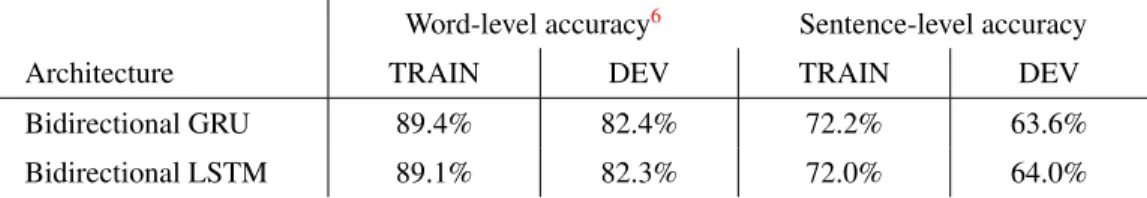
Given the large bias problem, the next task was to try a larger network. Korpusik (4) achieved good performance (92.1%weighted-average F1 score) in a similar food-related semantic labeling task using the same network structure as mine5 _{but with significantly more hidden units: 128 in} the embedding layer and 512 in the recurrent layer. Accordingly, I took the two best performing architectures from the first experiment (bidirectional GRU and bidirectional LSTM), and trained for 10 epochs with this much larger number of units. The results are summarized in Table2.

Word-level accuracy6 _{Sentence-level accuracy}

Architecture TRAIN DEV TRAIN DEV

Bidirectional GRU 89.4% 82.4% 72.2% 63.6%

Bidirectional LSTM 89.1% 82.3% 72.0% 64.0%

Table 2: Larger network experiment results (128 unit embedding layer, 512 unit recurrent layer).

While the larger NNs did achieve significantly higher accuracy than the initial networks on the TRAIN set, the improvement on the DEV set was relatively small (<1%improvement). Furthermore, as

4_{I expect human-level performance on this task to be close to}_100%_{accuracy, given that most people can}

read and follow recipes without issue.

5

Concretely, an embedding layer, followed by a bidirectional GRU, followed by a softmax layer, implemented in PyTorch

6

DEV word-level accuracy here is the best accuracy achieved by the model at the end of any epoch of training, as if early-stopping had been applied.

(4)

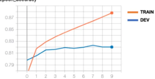
shown in Figure2, while DEV accuracy had plateaued, TRAIN accuracy was still improving, and would have likely gone up further if the model were trained for more than 10 epochs.

Figure 2: TRAIN and DEV accuracy of large Bidirectional LSTM model.

Accordingly, these results suggest that variance has become a bigger issue than bias for our model. 5.3 Addressing Variance

In an attempt to address the large variance issue, I ran some experiments testing dropout regularization, as well as increasing the number of recurrent layers. While there was some minor DEV performance improvement, it seemed like my model was stuck at a ceiling of∼83%word-level accuracy, similar to the baseline NYT model. The full results of these experiments are summarized in Tables6and7 in AppendixC.2.

5.4 Error Analysis

To investigate why I was having trouble addressing the variance issue, I did an error analysis on 50 randomly selected ingredient phrases that were incorrectly tagged by my best-performing model (2-layer Bidirectional LSTM with a 0.2 dropout rate). I discovered that68%of the errors were at least partially driven (and44%were solely driven) by incorrect labels provided by the dataset. While human-level performance on this task is expected to be high, because the NYT used a team of contractors to tag their dataset, the dataset was "inconsistent and incomplete" (2). Furthermore, some tags are a matter of judgement (e.g. should "extra-virgin" be tagged as a part of the name or a part of the comment for the ingredient "extra-virgin olive oil"), and these judgement calls appear to have been made inconsistently across many different contractors.

5.5 Manually Tagged Data

Rather than attempt to correct the many errors in the extremely large NYT dataset, I instead chose to generate a second dataset with more accurate and consistently applied labels, by manually tagging a small 3,000 example dataset myself (see Section3). This also had the benefit of more accurately reflecting the real-world distribution of recipes (whereas the NYT database only contained NYT recipes), so my experiment results would more likely reflect my model’s real-world performance. I used a randomly selected 1,000 example subset of this dataset as my new DEV set to evaluate performance on, and tried to use the remaining 2,000 examples to train my model in three different ways.

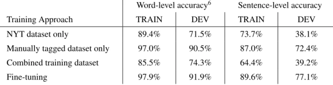
First, I tried to train my best performing model architecture so far (2-layer Bidirectional LSTM) using only these 2,000 examples, trying various dropout rates, for 50 epochs (the smaller training set with the same batch size meant I had to train for more epochs before the model converged). Second, I tried to train the same model using a combined dataset of both my original TRAIN dataset (from NYT) and these 2,000 examples, up-weighting the manually tagged examples by various amounts. Finally, I attempted to use transfer learning, first training the same model using just the large NYT dataset for 10 epochs, and then fine-tuning the model on my smaller manually-tagged dataset, training for 20 epochs. The best performance I achieved using each of these methods is compared against my previous best model (trained only on the NYT dataset) in Table3. Note that the DEV set mentioned

(5)

here is the new DEV set of manually tagged examples, which is why the NYT dataset only DEV performance is different from the previous tables.

Training Approach TRAIN DEV TRAIN DEV

NYT dataset only 89.4% 71.5% 73.7% 38.1%

Manually tagged dataset only 97.0% 90.5% 87.0% 72.4%

Combined training dataset 85.5% 74.3% 64.4% 39.2%

Fine-tuning 97.9% 91.9% 89.6% 77.1%

Table 3: Performance of various methods of incorporating manually tagged data.

Just training on the manually tagged dataset already significantly outperforms my previous model trained on the much larger NYT dataset, likely because the NYT dataset is extremely noisy, and comes from a different distribution than my new DEV set. Surprisingly, combining the NYT training dataset with the manually tagged dataset and up-weighting the manually tagged examples did worse, even for very high weights (e.g. 100); it’s possible that the model was hampered from learning due to the inconsistent tagging strategies observed in the NYT database, and this effect outweighed the benefit of many more training examples. The fine-tuning method performed the best of all three methods. This is possibly because the initial training phase allowed the model to learn good embeddings (and possibly rough tagging rules) for a larger set of ingredient phrase words, as the large NYT dataset had a much larger vocab size than the manually tagged dataset, while the fine-tuning phase was not hampered by the inconsistent tagging rules present in the NYT dataset.

For the full results of each set of experiments, see Tables8,9, and10in AppendixC.3. 5.6 Performance of Best Model

The best model across all experiments was a 2-layer Bidirectional LSTM model with 512-units in each recurrent layer and 128-units in the embedding layer, trained for 10 epochs on the NYT dataset with a 0.2 dropout rate and 20 epochs on the manually tagged dataset with a 0.6 dropout rate. It achieved a performance of91.9%word-level accuracy on the manually tagged DEV set.

The model performs particularly well on tagging quantities, does quite well on tagging unit words, and decently at tagging ingredient names. It struggles the most with the COMMENT and OTHER tags. This skewed performance is acceptable, as quantity, unit and ingredient information are the most important for most use cases (e.g. nutrition calculation). A more detailed discussion of the performance of the best model can be found in AppendixD.

6 Future Work

There are several avenues of work that I plan on exploring in the future:

1. Manually tag more dataDue to the time constraints of this project, I was only able to manually tag 3,000 examples - I hope to expand my dataset further later on.

2. Use pre-trained word embeddingsRather than use a trainable embedding layer, I’d like to try using a pre-trained word-embedding. I may also consider training my own embedding on a large corpus of recipes, as recipes have a fairly distinct distribution than a general text corpus; for example, recipes use a lot of ingredient names and cooking verbs that may be quite rare in a general text corpus.

3. Other architecturesKorpusik (4) mention achieving significant success by fine-tuning BERT with a token-classification layer on top - I’d like to try this approach on my problem domain as well.

(6)

References

[1] E. Greene, “Extracting structured data from recipes using conditional random fields,” Apr 2015. [Online]. Available: https://open.blogs.nytimes.com/2015/04/09/ extracting-structured-data-from-recipes-using-conditional-random-fields/

[2] E. Greene and A. Mckaig, “Our tagged ingredients data is now on github,” May 2017. [Online]. Available: https://open.nytimes.com/ our-tagged-ingredients-data-is-now-on-github-f96e42abaa1c

[3] M. Korpusik, “Spoken language understanding in a nutrition dialogue system,” Master’s thesis, MIT, 2015. [Online]. Available: https://groups.csail.mit.edu/sls/publications/2015/Korpusik_ SM-Thesis.pdf

[4] ——, “Deep learning for spoken dialogue systems: Application to nutrition,” Ph.D. dissertation, MIT, 2019. [Online]. Available: https://groups.csail.mit.edu/sls/publications/2019/Korpusik_ PhD-Thesis.pdf

[5] M. Abadi, A. Agarwal, P. Barham, E. Brevdo, Z. Chen, C. Citro, G. S. Corrado, A. Davis, J. Dean, M. Devin, S. Ghemawat, I. Goodfellow, A. Harp, G. Irving, M. Isard, Y. Jia, R. Jozefowicz, L. Kaiser, M. Kudlur, J. Levenberg, D. Mané, R. Monga, S. Moore, D. Murray, C. Olah, M. Schuster, J. Shlens, B. Steiner, I. Sutskever, K. Talwar, P. Tucker, V. Vanhoucke, V. Vasudevan, F. Viégas, O. Vinyals, P. Warden, M. Wattenberg, M. Wicke, Y. Yu, and X. Zheng, “TensorFlow: Large-scale machine learning on heterogeneous systems,” 2015, software available

from tensorflow.org. [Online]. Available:http://tensorflow.org/ [6] F. Cholletet al., “Keras,”https://keras.io, 2015.

[7] M. Lynch, “Crf ingredient phrase tagger.” [Online]. Available: https://github.com/mtlynch/ ingredient-phrase-tagger

A

Manual Tagging Tool

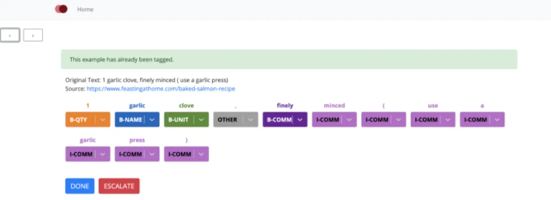
The manual example tagging tool I wrote made it significantly faster to generate examples. Examples were scrapped from recipes from a variety of popular online recipe websites usingthis python package, and were pre-tagged with my best-performing model trained on only the NYT dataset to speed up manual tagging.

A live version of the tagging tool can be accessedhere, and the code for the tagging tool can be found here. I’ve also included a screenshot of the tagging tool in Figure3.

(7)

B

Baseline

For the baseline model, I used the public New York Times linear-chain CRF model described in (1) and provided in theingredient-phrase-tagger github repo. Unfortunately, this repo had not been worked on for quite a while (last commit was in 2016), and would not run out of the box.

However, I found a fork of the repothat had been cleaned up, which I got to run with minor modifications (7). My code can be found in the github repohere.

The performance of the baseline model is summarized in Table11:

Dataset Word-level accuracy Sentence-level accuracy

TRAIN 87.8% 70.1%

DEV 83.6% 66.8%

TEST 84.2% 65.7%

Table 4: Baseline model performance.

C

Detailed Experiment Results

C.1 NN Architecture Search

Models used a 64-unit embedding layer, a 64-unit recurrent layer, and a softmax layer, and were trained for 10 epochs.

Word-level accuracy Sentence-level accuracy

Architecture TRAIN DEV TRAIN DEV

RNN 83.6% 80.4% 63.0% 59.6% Bidirectional RNN 85.7% 81.0% 66.6% 61.3% GRU 83.9% 80.5% 63.0% 59.6% Bidirectional GRU 86.1% 81.7% 67.5% 62.7% LSTM 83.7% 80.4% 63.5% 60.6% Bidirectional LSTM 85.8% 81.6% 67.1% 62.8%

Table 5: Architecture search experiment results.

C.2 Addressing Variance C.2.1 Regularization

Models used a 128-unit embedding layer, a 512-unit recurrent layer, and a softmax layer, and were trained for 10 epochs with various dropout rates using dropout regularization.

Architecture (Dropout Rate) TRAIN DEV TRAIN DEV

Bidirectional GRU (0.2) 88.0% 82.3% 70.0% 64.2%

Bidirectional GRU (0.4) 86.6% 82.6% 68.7% 64.4%

Bidirectional LSTM (0.2) 87.7% 82.2% 70.4% 64.7%

Bidirectional LSTM (0.4) 86.7% 82.7% 69.4% 65.2%

(8)

C.2.2 More Recurrent Layers

Models used a 128-unit embedding layer, 1 to 3 512-unit recurrent layers, and a softmax layer, and were trained for 10 epochs with various dropout rates using dropout regularization.

Word-level accuracy6 Sentence-level accuracy Architecture (# layers) [Dropout Rate] TRAIN DEV TRAIN DEV

Bidirectional GRU (2) [0] 91.3% 82.6% 76.3% 65.1% Bidirectional GRU (3) [0] 91.0% 82.5% 75.2% 65.2% Bidirectional LSTM (2) [0] 91.4% 82.6% 76.5% 65.3% Bidirectional LSTM (3) [0] 91.4% 82.8% 76.3% 65.0% Bidirectional LSTM (2) [0.2] 89.4% 83.0% 73.7% 67.2% Bidirectional LSTM (3) [0.2] 89.5% 82.8% 73.7% 67.0%

Table 7: Large network experiment results with multiple recurrent layers.

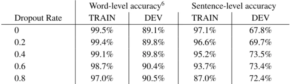
C.3 Incorporating Manually Tagged Data C.3.1 Using Only Manually Tagged Data

Models used a 128-unit embedding layer, 2 512-unit bidirectional LSTM recurrent layers, and a softmax layer, and were trained for 50 epochs using various dropout rates.

Dropout Rate TRAIN DEV TRAIN DEV

0 99.5% 89.1% 97.1% 67.8%

0.2 99.4% 89.8% 96.6% 69.7%

0.4 99.1% 89.8% 95.2% 73.5%

0.6 98.7% 90.4% 93.7% 73.4%

0.8 97.0% 90.5% 87.0% 72.4%

Table 8: Results using only manually tagged data to train model.

C.3.2 Combining NYT and Manually Tagged Data

Models used a 128-unit embedding layer, 2x 512-unit bidirectional LSTM recurrent layers, and a softmax layer, and were trained using a dropout rate of 0.2 for a total of 10 epochs.

Manually Tagged Data Weight TRAIN DEV TRAIN DEV

1 85.4% 73.6% 62.5% 37.6%

10 85.5% 74.3% 64.4% 39.2%

100 85.3% 74.3% 62.3% 38.7%

Table 9: Results using combined NYT and manually tagged data to train model.

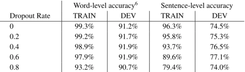
C.3.3 Fine-tuning

Models used a 128-unit embedding layer, 2 512-unit bidirectional LSTM recurrent layers, and a softmax layer, and were trained for 10 epochs on the NYT TRAIN dataset, and subsequently fine-tuned on the manually tagged dataset for 20 epochs. A variety of dropout rates were tested.

(9)

Dropout Rate TRAIN DEV TRAIN DEV

0 99.3% 91.2% 96.3% 74.5%

0.2 99.2% 91.7% 95.8% 75.3%

0.4 98.9% 91.9% 93.7% 76.5%

0.6 97.9% 91.9% 89.6% 77.1%

0.8 93.2% 90.7% 79.4% 74.0%

Table 10: Results training model first on NYT data, and then fine-tuned on manually tagged data.

D

Analysis of Best Model Performance

Figure 4: Confusion Matrix

TAG B-QTY I-QTY B-UNIT I-UNIT B-NAME I-NAME

F1 Score 97.5% 99.1% 96.3% 74.0% 91.4% 93.7%

TAG B-COMM I-COMM B-RANGE_END I-RANGE_END OTHER

F1 Score 84.2% 89.6% n/a n/a 85.0%

Table 11: Per-tag F1 scores.

The model performs extremely well on tagging beginnings and interiors of quantities, with near-perfect F1 scores - this is not surprising, given that almost all quantities are numeric, and most appearances of numeric characters are part of the quantity.

The model also does very well on identifying beginnings of units, but very poorly on identifying interiors of units, likely because most units are 1 word / token long, and thus the I-UNIT tag is quite rare. To address this we could add more training examples that include multi-word unit phrases (e.g. "1 28 oz can black beans").

The model achieves average performance on ingredient names - hopefully further expanding the manually tagged training set will further improve the performance on these two tags.

The COMMENT and OTHER tags are less relevant for the use case of this model, and are thus not a priority for improvement.

E

Bad Experiment Results Due Poor Shuffling Between Epochs

The initial architecture search and hyperparameter tuning experiments I ran were all tainted by improper shuffling of the training examples in between epochs7- this resulted in surprisingly poor performance on both TRAIN and DEV sets, well below the baseline model.

7

This was caused by a misunderstanding about howtf.data.Dataset.shuffleworked - I used a very small buffer size relative to my dataset size.

(10)

One interesting phenomenon I observed during these initial experiments was that the TRAIN accuracy reported during the last epoch ofmodel.fit) was significantly higher than the accuracy of the final model on the TRAIN set (>90%vs. <80%), which suggests that the model was adapting to the order of the examples, oscillating between weights that did well on each section of the examples. The results of these experiments have been included below for completeness.

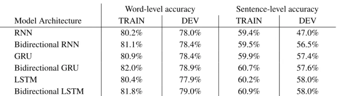
E.1 Architecture Search

Model Architecture TRAIN DEV TRAIN DEV

RNN 80.2% 78.0% 59.4% 47.0% Bidirectional RNN 81.1% 78.4% 59.5% 56.5% GRU 80.9% 78.4% 59.9% 57.4% Bidirectional GRU 82.0% 78.9% 60.7% 57.6% LSTM 80.4% 77.9% 60.2% 58.0% Bidirectional LSTM 81.8% 79.0% 60.9% 58.0%

Table 12: Architecture search experiment results (64 unit embedding layer, 64 unit recurrent layer).

E.2 Larger Network

Table 13: Larger network experiment results (128 unit embedding layer, 512 unit recurrent layer).

E.3 Dropout Regularization