Model Selection Through Sparse Maximum Likelihood Estimation for Multivariate Gaussian or Binary Data

(1)

Model Selection Through

Sparse Maximum Likelihood Estimation

for Multivariate Gaussian or Binary Data

Onureena Banerjee [email protected]

Laurent El Ghaoui [email protected]

EECS Department

University of California, Berkeley Berkeley, CA 94720 USA

Alexandre d’Aspremont [email protected]

ORFE Department Princeton University Princeton, NJ 08544 USA

Editor: Leslie Pack Kaelbling

Abstract

We consider the problem of estimating the parameters of a Gaussian or binary distribution in such a way that the resulting undirected graphical model is sparse. Our approach is to solve a maximum likelihood problem with an added ℓ1-norm penalty term. The

problem as formulated is convex but the memory requirements and complexity of existing interior point methods are prohibitive for problems with more than tens of nodes. We present two new algorithms for solving problems with at least a thousand nodes in the Gaussian case. Our first algorithm uses block coordinate descent, and can be interpreted as recursiveℓ₁-norm penalized regression. Our second algorithm, based on Nesterov’s first order method, yields a complexity estimate with a better dependence on problem size than existing interior point methods. Using a log determinant relaxation of the log partition function (Wainwright and Jordan [2006]), we show that these same algorithms can be used to solve an approximate sparse maximum likelihood problem for the binary case. We test our algorithms on synthetic data, as well as on gene expression and senate voting records data.

Keywords: Model Selection, Maximum Likelihood Estimation, Convex Optimization, Gaussian Graphical Model, Binary Data

(2)

1. Introduction

Undirected graphical models offer a way to describe and explain the relationships among a set of variables, a central element of multivariate data analysis. The principle of parsimony dictates that we should select the simplest graphical model that adequately explains the data. In this paper weconsider practical ways of implementing the following approach to finding such a model: given a set of data, we solve a maximum likelihood problem with an addedℓ1-norm penalty to make the resulting graph as sparse as possible.

Many authors have studied a variety of related ideas. In the Gaussian case, model selection involves finding the pattern of zeros in the inverse covariance matrix, since these zeros correspond to conditional independencies among the variables. Traditionally, a greedy forward-backward search algorithm is used to determine the zero pattern [e.g., Lauritzen, 1996]. However, this is computationally infeasible for data with even a moderate number of variables. Li and Gui [2005] introduce a gradient descent algorithm in which they account for the sparsity of the inverse covariance matrix by defining a loss function that is the negative of the log likelihood function. Recently, Huang et al. [2005] considered penalized maximum likelihood estimation, and Dahl et al. [2006] proposed a set of large scale methods for problems where a sparsity pattern for the inverse covariance is given and one must estimate the nonzero elements of the matrix.

Another way to estimate the graphical model is to find the set of neighbors of each node in the graph by regressing that variable against the remaining variables. In this vein, Dobra and West [2004] employ a stochastic algorithm to manage tens of thousands of variables. There has also been a great deal of interest in using ℓ1-norm penalties in statistical

appli-cations. d’Aspremont et al. [2004] apply anℓ1 norm penalty to sparse principle component

analysis. Directly related to our problem is the use of the Lasso of Tibshirani [1996] to ob-tain a very short list of neighbors for each node in the graph. Meinshausen and B¨uhlmann [2006] study this approach in detail, and show that the resulting estimator is consistent, even for high-dimensional graphs.

The problem formulation for Gaussian data, therefore, is simple. The difficulty lies in its computation. Although the problem is convex, it is non-smooth and has an unbounded constraint set. As we shall see, the resulting complexity for existing interior point methods is _O(p6_{), where}_p _{is the number of variables in the distribution. In addition, interior point}

methods require that at each step we compute and store a Hessian of size O(p2). The memory requirements and complexity are thus prohibitive for O(p) higher than the tens. Specialized algorithms are needed to handle larger problems.

The remainder of the paper is organized as follows. We begin by considering Gaussian data. In Section 2 we set up the problem, derive its dual, discuss properties of the solution and how heavily to weight the ℓ1-norm penalty in our problem. In Section 3 we present a

provably convergent block coordinate descent algorithm that can be interpreted as recursive

(3)

on Nesterov’s recent work on non-smooth optimization, and give a rigorous complexity analysis with better dependence on problem size than interior point methods. In Section??

we show that the algorithms we developed for the Gaussian case can also be used to solve an approximate sparse maximum likelihood problem for multivariate binary data, using a log determinant relaxation for the log partition function given by Wainwright and Jordan [2006]. In Section 6, we test our methods on synthetic as well as gene expression and senate voting records data.

2. Problem Formulation

In this section we set up the sparse maximum likelihood problem for Gaussian data, derive its dual, and discuss some of its properties.

2.1 Problem setup.

Suppose we are givennsamples independently drawn from ap-variate Gaussian distribution:

y(1), . . . , y(n) _{∼ N}_(Σ

p, µ), where the covariance matrix Σ is to be estimated. Let S denote

the second moment matrix about the mean:

S:= 1 n n X k=1 (y(k)₋µ)(y(k)₋µ)T.

Let ˆΣ−1 _{denote our estimate of the inverse covariance matrix. Our estimator takes the}

form:

ˆ

Σ−1= arg max

X≻0log detX−trace(SX)−λkXk1. (1)

Here, _kX_k1 denotes the sum of the absolute values of the elements of the positive definite

matrixX.

The scalar parameter λ controls the size of the penalty. The penalty term is a proxy for the number of nonzero elements in X, and is often used – albiet with vector, not matrix, variables – in regression techniques, such as the Lasso.

In the case where S ≻0, the classical maximum likelihood estimate is recovered for λ= 0. However, when the number of samples n is small compared to the number of variables p, the second moment matrix may not be invertible. In such cases, for λ >0, our estimator performs some regularization so that our estimate ˆΣ is always invertible, no matter how small the ratio of samples to variables is.

(4)

Even in cases where we have enough samples so that S ≻ 0, the inverse S−1 may not be sparse, even if there are many conditional independencies among the variables in the distribution. By trading off maximality of the log likelihood for sparsity, we hope to find a very sparse solution that still adequately explains the data. A larger value ofλcorresponds to a sparser solution that fits the data less well. A smallerλcorresponds to a solution that fits the data well but is less sparse. The choice ofλis therefore an important issue that will be examined in detail in Section 2.3.

2.2 The dual problem and bounds on the solution.

We can write (1) as

max

X≻0kUmink∞≤λ

log detX+ trace(X, S+U)

where_kU_k∞denotes the maximum absolute value element of the symmetric matrixU. This corresponds to seeking an estimate with the maximum worst-case log likelihood, over all additive perturbations of the second moment matrixS. A similar robustness interpretation can be made for a number of estimation problems, such as support vector machines for classification.

We can obtain the dual problem by exchanging the max and the min. The resulting inner problem inX can be solved analytically by setting the gradient of the objective to zero and solving forX. The result is

min kUk∞≤λ

−log det(S+U)₋p

where the primal and dual variables are related as: X = (S +U)−1_{. Note that the log}

determinant function acts a log barrier, creating an implicit constraint thatS+U _≻0. To write things neatly, let W =S+U. Then the dual of our sparse maximum likelihood problem is

ˆ

Σ := max{log detW :kW −Sk∞≤λ}. (2)

Observe that the dual problem (1) estimates the covariance matrix while the primal problem estimates its inverse. We also observe that the diagonal elements of the solution are Σkk=

Skk+λfor allk.

The following theorem shows that adding the ℓ1-norm penalty regularlizes the solution. Theorem 1 For everyλ >0, the optimal solution to (1) is unique, with bounded eigenval-ues:

p λ ≥ kΣˆ

−1_k

2 ≥(kSk2+λp)−1.

(5)

The dual problem (2) is smooth and convex. When p(p+ 1)/2 is in the low hundreds, the problem can be solved by existing software that uses an interior point method [e.g., Vandenberghe et al., 1998]. The complexity to compute an ǫ-suboptimal solution using such second-order methods, however, is _O(p6_log(1_/ǫ_{)), making them infeasible when}_p _is

larger than the tens.

A related problem, solved by Dahl et al. [2006], is to compute a maximum likelihood estimate of the covariance matrix when the sparsity structure of the inverse is known in advance. This is accomplished by adding constraints to (1) of the form: Xij = 0 for all pairs (i, j)

in some specified set. Our constraint set is unbounded as we hope to uncover the sparsity structure automatically, starting with a dense second moment matrixS.

2.3 Choice of penalty parameter.

Consider the true, unknown graphical model for a given distribution. This graph has p

nodes, and an edge between nodesk and j is missing if variables k and j are independent conditional on the rest of the variables. For a given node k, let Ck denote its connectivity

component: the set of all nodes that are connected to nodek through some chain of edges. In particular, if nodej6∈ Ck, then variablesj and k are independent.

We would like to choose the penalty parameterλso that, for finite samples, the probability of error in estimating the graphical model is controlled. To this end, we can adapt the work of Meinshausen and B¨uhlmann [2006] as follows. Let ˆCλ

k denote our estimate of

the connectivity component of node k. In the context of our optimization problem, this corresponds to the entries of rowk in ˆΣ that are nonzero.

Let α be a given level in [0,1]. Consider the following choice for the penalty parameter in (1): λ(α) := (max i>j σˆiσˆj) tn−2(α/2p2) q n−2 +t2_n₋₂(α/2p2₎ (3)

wheretn−2(α) denotes the (100−α)% point of the Student’s t-distribution forn−2 degrees

of freedom, and ˆσi is the empirical variance of variable i. Then we can prove the following

theorem:

Theorem 2 Usingλ(α) the penalty parameter in (1), for any fixed levelα,

P(∃k∈ {1, . . . , p}: ˆC_kλ 6⊆Ck)≤α.

Observe that, for a fixed problem size p, as the number of samples n increases to infinity, the penalty parameter λ(α) decreases to zero. Thus, asymptotically we recover the

(6)

clas-sical maximum likelihood estimate, S, which in turn converges in probability to the true covariance Σ.

3. Block Coordinate Descent Algorithm

In this section we present an algorithm for solving (2) that uses block coordinate descent.

3.1 Algorithm description.

We begin by detailing the algorithm. For any symmetric matrix A, let A_\j\k denote the

matrix produced by removing row k and column j. Let Aj denote column j with the

diagonal element Ajj removed. The plan is to optimize over one row and column of the

variable matrixW at a time, and to repeatedly sweep through all columns until we achieve convergence.

Initialize: W(0) :=S+λI For k_≥0

1. For j= 1, . . . , p

(a) LetW(j−1) _{denote the current iterate. Solve the quadratic program}

ˆ y:= arg min y {y T₍_W(j−1) \j\j ) −1_y _:_k_y₋_S jk∞≤λ} (4)

(b) Update rule: W(j) _is_W(j−1) _{with column/row} _W

j replaced by ˆy.

2. Let ˆW(0)_:=_W(p)_.

3. After each sweep through all columns, check the convergence condition. Convergence occurs when

trace(( ˆW(0))−1S)₋p+λ_k( ˆW(0))−1_k1 ≤ǫ. (5)

3.2 Convergence and property of solution.

Using Schur complements, we can prove convergence:

Theorem 3 The block coordinate descent algorithm described above converges, acheiving an ǫ-suboptimal solution to (2). In particular, the iterates produced by the algorithm are strictly positive definite: each time we sweep through the columns, W(j)_≻₀ _{for all} _j_.

(7)

The proof of Theorem 3 sheds some interesting light on the solution to problem (1). In particular, we can use this method to show that the solution has the following property:

Theorem 4 Fix any k∈ {1, . . . , p}. If λ≥ |Skj| for all j 6=k, then column and row k of

the solution Σˆ to (2) are zero, excluding the diagonal element.

This means that, for a given second moment matrixS, ifλis chosen such that the condition in Theorem 4 is met for some column k, then the sparse maximum likelihood method esti-mates variable kto be independent of all other variables in the distribution. In particular, Theorem 4 implies that if λ ≥ |Skj| for all k > j, then (1) estimates all variables in the

distribution to be pairwise independent.

Using the work of Luo and Tseng [1992], it may be possible to show that the local conver-gence rate of this method is at least linear. In practice we have found that a small number of sweeps through all columns, independent of problem size p, is sufficient to achieve con-vergence. For a fixed number of K sweeps, the cost of the method is O(Kp4), since each iteration costs O(p3).

3.3 Interpretation as recursive penalized regression.

The dual of (4) is min x x T_W(j−1) \j\j x−S T j x+λkxk1. (6)

Strong duality obtains so that problems (6) and (4) are equivalent. If we let Qdenote the square root ofW_\(_jj_\−_j1), andb:= 1₂Q−1Sj, then we can write (6) as

min

x kQx−bk 2

2+λkxk1. (7)

The problem (7) is a penalized least-squares problems, known as the Lasso. IfW_\(_jj_\−_j1) were the j-th principal minor of the sample covariance S, then (7) would be equivalent to a penalized regression of variable j against all others. Thus, the approach is reminiscent of the approach explored by Meinshausen and B¨uhlmann [2006], but there are two differences. First, we begin with some regularization and, as a consequence, each penalized regression problem has a unique solution. Second, and more importantly, we update the problem data after each regression: except at the very first update,W_\(_jj_\−_j1) is never a minor of S. In this sense, the coordinate descent method can be interpreted as a recursive Lasso.

(8)

4. Nesterov’s First Order Method

In this section we apply the recent results due to Nesterov [2005] to obtain a first order algo-rithm for solving (1) with lower memory requirements and a rigorous complexity estimate with a better dependence on problem size than those offered by interior point methods. Our purpose is not to obtain another algorithm, as we have found that the block coordinate descent is fairly efficient; rather, we seek to use Nesterov’s formalism to derive a rigorous complexity estimate for the problem, improved over that offered by interior-point methods. As we will see, Nesterov’s framework allows us to obtain an algorithm that has a complexity of O(p4.5/ǫ), where ǫ >0 is the desired accuracy on the objective of problem (1). This is in contrast to the complexity of interior-point methods, O(p6log(1/ǫ)). Thus, Nesterov’s method provides a much better dependence on problem size and lower memory requirements at the expense of a degraded dependence on accuracy.

4.1 Idea of Nesterov’s method.

Nesterov’s method applies to a class of non-smooth, convex optimization problems of the form

min

x {f(x) :x∈Q1} (8)

where the objective function can be written as

f(x) = ˆf(x) + max

u {hAx, ui2 :u∈Q2}.

Here, Q1 and Q2 are bounded, closed, convex sets, ˆf(x) is differentiable (with a

Lipschitz-continuous gradient) and convex on Q1, and A is a linear operator. The challenge is to

write our problem in the appropriate form and choose associated functions and parameters in such a way as to obtain the best possible complexity estimate, by applying general results obtained by Nesterov [2005].

Observe that we can write (1) in the form (8) if we impose bounds on the eigenvalues of the solution, X. To this end, we let

Q1:={x:aI X bI} Q2:={u:kuk∞≤λ}

(9)

where the constantsa, b are given such that b > a >0. By Theorem 1, we know that such bounds always exist. We also define ˆf(x) :=₋log detx+_hS, x_i, andA:=λI.

ToQ1 and Q2, we associate norms and continuous, strongly convex functions, called

(9)

d1(x) = −log detx + logb. For Q2, we choose the Frobenius norm again, and a

prox-functiond2(x) =kuk2F/2.

The method applies a smoothing technique to the non-smooth problem (8), which replaces the objective of the original problem, f(x), by a penalized function involving the prox-functiond2(u):

˜

f(x) = ˆf(x) + max

u∈Q2{h

Ax, u_{i −}µd2(u)}. (10)

The above function turns out to be a smooth uniform approximation to f everywhere. It is differentiable, convex onQ1, and a has a Lipschitz-continuous gradient, with a constant L that can be computed as detailed below. A specific gradient scheme is then applied to this smooth approximation, with convergence rate O(L/ǫ).

4.2 Algorithm and complexity estimate.

To detail the algorithm and compute the complexity, we must first calculate some pa-rameters corresponding to our definitions and choices above. First, the strong convexity parameter ford1(x) onQ1 isσ1 = 1/b2, in the sense that

∇2d1(X)[H, H] = trace(X−1HX−1H)≥b−2kHk2F

for every symmetricH. Furthermore, the center of the setQ1 isx0:= arg minx∈Q1d1(x) =

bI, and satisfies d1(x0) = 0. With our choice, we have D1 := maxx∈Q1 d1(x) =plog(b/a). Similarly, the strong convexity parameter ford2(u) onQ2 isσ2 := 1, and we have

D2 := max u∈Q2

d2(U) =p2/2.

With this choice, the center of the set Q2 is u0 := arg minu∈Q2d2(u) = 0.

For a desired accuracy ǫ, we set the smoothness parameter µ:= ǫ/2D2, and set x0 = bI.

The algorithm proceeds as follows:

For k≥0 do

1. Compute ∇f˜(xk) =−x−1+S+u∗(xk), whereu∗(x) solves (10).

2. Find yk= arg miny{h∇f˜(xk), y−xki+₂1L(ǫ)ky−xkk2F : y∈Q1}.

3. Find zk = arg minx{L_σ(ǫ)

1 d1(X) +

Pk

(10)

4. Updatexk= _k₊₃2 zk+k_k+1₊₃yk.

In our case, the Lipschitz constant for the gradient of our smooth approximation to the objective function is

L(ǫ) :=M +D2kAk2/(2σ2ǫ)

where M := 1/a2 is the Lipschitz constant for the gradient of ˜f, and the norm kAk is induced by the Frobenius norm, and is equal toλ.

The algorithm is guaranteed to produce an ǫ-suboptimal solution after a number of steps not exceeding N(ǫ) := 4_kA_k r D1D2 σ1σ2 · 1 ǫ + q M D1 σ1ǫ = (κp(logκ))(4p1.5aλ/√2 +√ǫp)/ǫ. (11)

whereκ=b/a is a bound on the condition number of the solution.

Now we are ready to estimate the complexity of the algorithm. For Step 1, the gradient of the smooth approximation is computed in closed form by taking the inverse of x. Step 2 essentially amounts to projecting on Q1, and requires that we solve an eigenvalue problem.

The same is true for Step 3. In fact, each iteration costs O(p3). The number of iterations necessary to achieve an objective with absolute accuracy less than ǫ is given in (11) by

N(ǫ) =O(p1.5_/ǫ_{). Thus, if the condition number} _κ _{is fixed in advance, the complexity of}

the algorithm isO(p4.5_/ǫ_).

5. Binary Variables: Approximate Sparse Maximum Likelihood Estimation

In this section, we consider the problem of estimating an undirected graphical model for multivariate binary data. Recently, Wainwright et al. [2006] applied anℓ1-norm penalty to

the logistic regression problem to obtain a binary version of the high-dimensional consistency results of Meinshausen and B¨uhlmann [2006]. We apply the log determinant relaxation of Wainwright and Jordan [2006] to formulate an approximate sparse maximum likelihood (ASML) problem for estimating the parameters in a multivariate binary distribution. We show that the resulting problem is the same as the Gaussian sparse maximum likelihood (SML) problem, and that we can therefore apply our previously-developed algorithms to sparse model selection in a binary setting.

(11)

Consider a distribution made up of p binary random variables. Usingn data samples, we wish to estimate the structure of the distribution. The logistic model of this distribution is

p(x;θ) = exp_{ p X i=1 θixi+ p−1 X i=1 p X j=i+1 θijxixj−A(θ)} (12) where A(θ) = log X x∈Xp exp_{ p X i=1 θixi+ p−1 X i=1 p X j=i+1 θijxixj} (13)

is the log partition function.

The sparse maximum likelihood problem in this case is to maximize (12) with an added

ℓ1-norm penalty on terms θkj. Specifically, in the undirected graphical model, an edge

between nodesk and j is missing ifθkj = 0.

A well-known difficulty is that the log partition function has too many terms in its outer sum to compute. However, if we use the log determinant relaxation for the log partition function developed by Wainwright and Jordan [2006], we can obtain an approximate sparse maximum likelihood (ASML) estimate. We shall set up the problem in the next section.

5.1 Problem formulation.

Let’s begin with some notation. Lettingd:=p(p+ 1)/2, define the map R:Rd_→Sp+1 _as

follows: R(θ) =      0 θ1 θ2 . . . θp θ1 0 θ12 . . . θ1p .. . θp θ1p θ2p . . . 0     

Suppose that our n samples are z(1₎_{, . . . , z}(n) _{∈ {−}₁_,₊₁_}p_{. Let ¯}_z

i and ¯zij denote sample

mean and second moments. The sparse maximum likelihood problem is ˆ

θ_{exact := arg max}

θ

1

2hR(θ), R(¯z)i −A(θ)−λkθk1. (14) Finally define the constant vectorm= (1,4₃, . . . ,4₃)∈Rp+1. Wainwright and Jordan [2006] give an upper bound on the log partition function as the solution to the following variational problem:

A(θ)_≤maxµ1₂log det(R(µ) + diag(m)) +hθ, µi

= 1₂ _·maxµlog det(R(µ) + diag(m)) +hR(θ), R(µ)i.

(12)

If we use the bound (15) in our sparse maximum likelihood problem (14), we won’t be able to extract an optimizing argument ˆθ. Our first step, therefore, will be to rewrite the bound in a form that will allow this.

Lemma 5 We can rewrite the bound (15) as

A(θ)_≤ p 2log( eπ 2 )− 1 2(p+ 1)− 1 2 · {maxν ν T_m_{+ log det(} −(R(θ) +diag(ν))). (16)

Using this version of the bound (15), we have the following theorem.

Theorem 6 Using the upper bound on the log partition function given in (16), the approx-imate sparse maximum likelihood problem has the following solution:

ˆ

θk= ¯µk

ˆ

θkj =−(ˆΓ)−kj1

(17)

where the matrix Γˆ is the solution to the following problem, related to (2):

ˆ

Γ := arg max_{log detW :Wkk=Skk+

1

3, |Wkj−Skj| ≤λ}. (18)

Here,S is defined as before:

S = 1 n n X k=1 (z(k)₋_µ_¯₎₍_z(k)₋_µ_¯₎T

where ¯µ is the vector of sample means ¯zi.

In particular, this means that we can reuse the algorithms developed in Sections 3 and

?? for problems with binary variables. The relaxation (15) is the simplest one offered by Wainwright and Jordan [2006]. The relaxation can be tightened by adding linear constraints on the variableµ.

5.2 Penalty parameter choice for binary variables.

For the choice of the penalty parameter λ, we can derive a formula analogous to (3). Consider the choice

λ(α_{)bin :=} (χ

2₍_α/₂_p2_,₁₎₎1 2 (mini>jσˆiσˆj)√n

(13)

where χ2(α,1) is the (100 −α)% point of the chi-square distribution for one degree of freedom. Since our variables take on values in {−1,1}, the empirical variances are of the form:

ˆ

σ_i2= 1₋µ¯2_i.

Using (19), we have the following binary version of Theorem 2:

Theorem 7 With (19) chosen as the penalty parameter in the approximate sparse maxi-mum likelihood problem, for a fixed level α,

P(_∃k_{∈ {}1, . . . , p_}: ˆC_kλ _6⊆Ck)≤α.

6. Numerical Results

In this section we present the results of some numerical experiments, both on synthetic and real data.

6.1 Synthetic experiments.

Synthetic experiments require that we generate underlying sparse inverse covariance matri-ces. To this end, we first randomly choose a diagonal matrix with positive diagonal entries. A given number of nonzeros are inserted in the matrix at random locations symmetrically. Positive definiteness is ensured by adding a multiple of the identity to the matrix if needed. The multiple is chosen to be only as large as necessary for inversion with no errors.

6.1.1 Sparsity and thresholding.

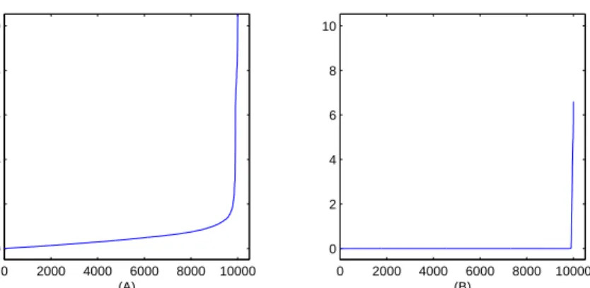
A very simple approach to obtaining a sparse estimate of the inverse covariance matrix would be to apply a threshold to the inverse empirical covariance matrix, S−1. However, even whenS is easily invertible, it can be difficult to select a threshold level. We solved a synthetic problem of size p = 100 where the true concentration matrix density was set to

δ= 0.1. Drawingn= 200 samples, we plot in Figure (1) the sorted absolute value elements of S−1 on the left and ˆΣ−1 on the right.

It is clearly easier to choose a threshold level for the SML estimate. Applying a threshold to eitherS−1 or ˆΣ−1would decrease the log likelihood of the estimate by an unknown amount. We only observe that to preserve positive definiteness, the threshold leveltmust satisfy the bound

t≤ min kvk1≤1

(14)

0 2000 4000 6000 8000 10000 0 2 4 6 8 10 (A) 0 2000 4000 6000 8000 10000 0 2 4 6 8 10 (B)

Figure 1: Sorted absolute value of elements of (A) S−1 and (B) ˆΣ−1. The solution ˆΣ−1 to (1) is un-thresholded.

6.1.2 Recovering structure.

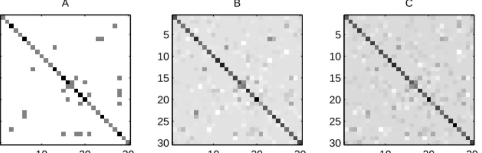
We begin with a small experiment to test the ability of the method to recover the sparse structure of an underlying covariance matrix. Figure 2 (A) shows a sparse inverse covariance matrix of size p = 30. Figure 2 (B) displays a corresponding S−1_{, using} _n _{= 60 samples.}

Figure 2 (C) displays the solution to (1) for λ= 0.1. The value of the penalty parameter here is chosen arbitrarily, and the solution is not thresholded. Nevertheless, we can still pick out features that were present in the true underlying inverse covariance matrix.

A 10 20 30 5 10 15 20 25 30 B 10 20 30 5 10 15 20 25 30 C 10 20 30 5 10 15 20 25 30

Figure 2: Recovering the sparsity pattern. We plot (A) the original inverse covariance matrix Σ−1, (B) the noisy sample inverse S−1, and (C) the solution to problem (1) forλ= 0.1.

Using the same underlying inverse covariance matrix, we repeat the experiment using smaller sample sizes. We solve (1) for n = 30 and n = 20 using the same arbitrarily chosen penalty parameter value λ = 0.1, and display the solutions in Figure (3). As ex-pected, our ability to pick out features of the true inverse covariance matrix diminishes with the number of samples. This is an added reason to choose a larger value ofλwhen we have fewer samples, as in (3).

(15)

A 10 20 30 5 10 15 20 25 30 B 10 20 30 5 10 15 20 25 30 C 10 20 30 5 10 15 20 25 30

Figure 3: Recovering the sparsity pattern for small sample size. We plot (A) the original inverse covariance matrix Σ−1, (B) the solution to problem (1) for n = 30 and (C) the solution for n= 20. A penalty parameter of λ= 0.1 is used for (B) and (C). 0 0.1 0.2 0.3 0.4 0.5 0.6 0.7 −0.4 −0.2 0 0.2 0.4 0.6 0.8 1 ˆ Σ − 1 ij λ 0 0.05 0.1 0.15 0.2 0.25 0.3 0.35 0.4 0.45 0.5 −0.7 −0.6 −0.5 −0.4 −0.3 −0.2 −0.1 0 0.1 0.2 0.3 λ ˆ Σ − 1 ij

Figure 4: Path following: elements of solution to (1) asλincreases. Red lines correspond to elements that are zero in the true inverse covariance matrix; blue lines correspond to true nonzeros. Vertical lines mark a range of λvalues using which we recover the sparsity pattern exactly.

6.1.3 Path following experiments.

Figure (4) shows two path following examples. We solve two randomly generated problems of size p = 5 and n = 100 samples. The red lines correspond to elements of the solution that are zero in the true underlying inverse covariance matrix. The blue lines correspond to true nonzeros. The vertical lines mark ranges of λ for which we recover the correct sparsity pattern exactly. Note that, by Theorem 4, for λvalues greater than those shown, the solution will be diagonal.

(16)

−0.50 0 0.5 1 1 2 3 4 5 6 7 E rr or (i n % ) log(λ/σ)

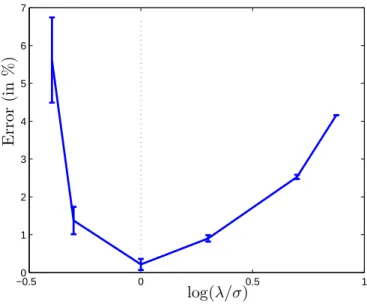
Figure 5: Recovering sparsity pattern in a matrix with added uniform noise of sizeσ= 0.1. We plot the average percentage or misclassified entries as a function of log(λ/σ).

On a related note, we observe that (1) also works well in recovering the sparsity pattern of a matrix masked by noise. The following experiment illustrates this observation. We generate a sparse inverse covariance matrix of sizep= 50 as described above. Then, instead of using an empirical covariance S as input to (1), we useS= (Σ−1₊_V₎−1_{, where}_V _{is a randomly}

generated uniform noise of sizeσ= 0.1. We then solve (1) for various values of the penalty parameterλ.

In figure 5, for a each of value ofλshown, we randomly selected 10 sample covariance ma-tricesSof sizep= 50 and computed the number of misclassified zeros and nonzero elements in the solution to (1). We plot the average percentage of errors (number of misclassified zeros plus misclassified nonzeros divided by p2), as well as error bars corresponding to one standard deviation. As shown, the error rate is nearly zero on average when the penalty is set to equal the noise level σ.

6.1.4 CPU times versus problem size.

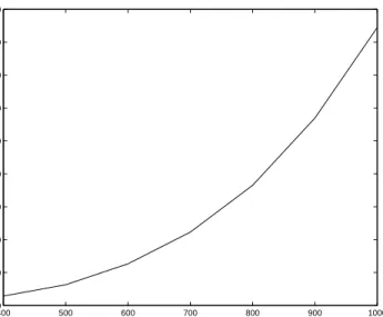
For a sense of the practical performance of the Nesterov method and the block coordinate descent method, we randomly selected 10 sample covariance matricesS for problem sizesp

ranging from 400 to 1000.In each case, the number of samples nwas chosen to be about a third ofp. In figure 6 we plot the average CPU time to achieve a duality gap ofǫ= 1. CPU times were computed using an AMD Athlon 64 2.20Ghz processor with 1.96GB of RAM.

(17)

400 500 600 700 800 900 1000 0 1000 2000 3000 4000 5000 6000 7000 8000 9000 Problem size p

Average CPU times in seconds

Figure 6: Average CPU times vs. problem size using block coordinate descent. We plot the average CPU time (in seconds) to reach a gap ofǫ= 0.1 versus problem sizep.

As shown, we are typically able to solve a problem of size p= 1000 in about two and half hours.

6.1.5 Performance as a binary classifier.

In this section we numerically examine the ability of the sparse maximum likelihood (SML) method to correctly classify elements of the inverse covariance matrix as zero or nonzero. For comparision, we will use the Lasso estimate of Meinshausen and B¨uhlmann [2006], which has been shown to perform extremely well. The Lasso regresses each variable against all others one at a time. Upon obtaining a solution θ(k) _{for each variable} _k_{, one can estimate}

sparsity in one of two ways: either by declaring an element ˆΣij nonzero if both θi(k) 6= 0

and θ(_jk) ₆= 0 (Lasso-AND) or, less conservatively, if either of those quantities is nonzero (Lasso-OR).

As noted previously, Meinshausen and B¨uhlmann [2006] have also derived a formula for choosing their penalty parameter. Both the SML and Lasso penalty parameter formulas depend on a chosen levelα, which is a bound on the same error probability for each method. For these experiments, we set α= 0.05.

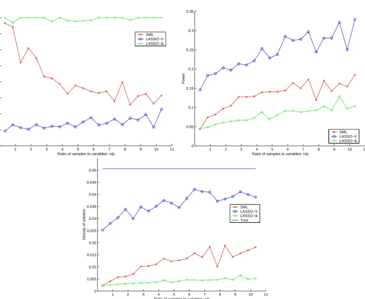
In the following experiments, we fixed the problem size p at 30 and generated sparse un-derlying inverse covariance matrices as described above. We varied the number of samples

n from 10 to 310. For each value of n shown, we ran 30 trials in which we estimated the sparsity pattern of the inverse covariance matrix using the SML, Lasso-OR, and Lasso-AND

(18)

1 2 3 4 5 6 7 8 9 10 11 0.2 0.3 0.4 0.5 0.6 0.7 0.8 0.9 1

Positive predictive value

Ratio of samples to variables: n/p

SML LASSO−V LASSO−& 1 2 3 4 5 6 7 8 9 10 11 0 0.05 0.1 0.15 0.2 0.25 0.3 0.35 Power

SML LASSO−V LASSO−& 1 2 3 4 5 6 7 8 9 10 11 0 0.005 0.01 0.015 0.02 0.025 0.03 0.035 0.04 0.045 0.05 Density of solution

SML LASSO−V LASSO−& True

Figure 7: Classifying zeros and nonzeros for a true density ofδ = 0.05. We plot the positive predictive value, the power, and the estimated density using SML, Lasso-OR and Lasso-AND.

methods. We then recorded the average number of nonzeros estimated by each method, and the average number of entries correctly identified as nonzero (true positives).

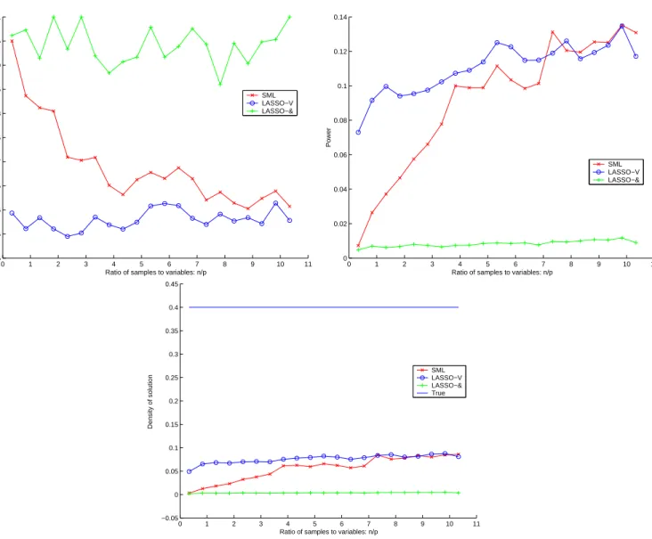
We show two sets of plots. Figure (7) corresponds to experiments where the true density was set to be low,δ= 0.05. We plot the power (proportion of correctly identified nonzeros), positive predictive value (proportion of estimated nonzeros that are correct), and the density estimated by each method. Figure (8) corresponds to experiments where the true density was set to be high,δ = 0.40, and we plot the same three quantities.

(19)

0 1 2 3 4 5 6 7 8 9 10 11 0.5 0.55 0.6 0.65 0.7 0.75 0.8 0.85 0.9 0.95 1

Positive predictive value

SML LASSO−V LASSO−& 0 1 2 3 4 5 6 7 8 9 10 11 0 0.02 0.04 0.06 0.08 0.1 0.12 0.14 Power

SML LASSO−V LASSO−& 0 1 2 3 4 5 6 7 8 9 10 11 −0.05 0 0.05 0.1 0.15 0.2 0.25 0.3 0.35 0.4 0.45 Density of solution

SML LASSO−V LASSO−& True

Figure 8: Classifying zeros and nonzeros for a true density ofδ = 0.40. We plot the positive predictive value, the power, and the estimated density using SML, Lasso-OR and Lasso-AND.

Meinshausen and B¨uhlmann [2006] report that, asymptotically, Lasso-AND and Lasso-OR yield the same estimate of the sparsity pattern of the inverse covariance matrix. At a finite number of samples, the SML method seems to fall in in between the two methods in terms of power, positive predictive value, and the density of the estimate. It typically offers, on average, the lowest total number of errors, tied with either Lasso-AND or Lasso-OR. Among the two Lasso methods, it would seem that if the true density is very low, it is slightly better to use the more conservative Lasso-AND. If the density is higher, it may be better to use Lasso-OR. When the true density is unknown, we can achieve an accuracy comparable to

(20)

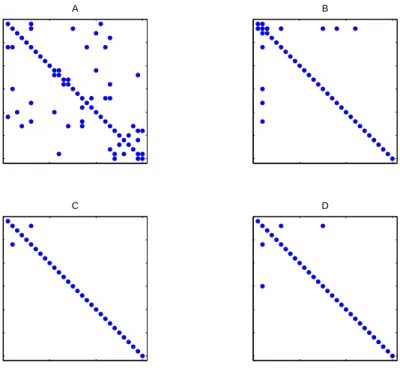
the better choice among the Lasso methods by computing the SML estimate. Figure (9) shows one example of sparsity pattern recovery when the true density is low.

A B

C D

Figure 9: Comparing sparsity pattern recovery to the Lasso. (A) true covariance (B) Lasso-OR (C) Lasso-AND (D) SML.

The Lasso and SML methods have a comparable computational complexity. However, unlike the Lasso, the SML method is not parallelizable. Parallelization would render the Lasso a more computationally attractive choice, since each variable can regressed against all other separately, at an individual cost of O(p3). In exchange, SML can offer a more accurate estimate of the sparsity pattern, as well as a well-conditioned estimate of the covariance matrix itself.

6.2 Gene expression and U.S. Senate voting records data.

We tested our algorithms on three sets of data: two gene expression data sets, as well as US Senate voting records. In this section we briefly explore the resulting graphical models.

(21)

6.2.1 Rosetta Inpharmatics compendium.

We applied our algorithms to the Rosetta Inpharmatics Compendium of gene expression profiles described by Hughes et al. [2000]. The 300 experiment compendium contains n= 253 samples with p = 6136 variables. With a view towards obtaining a very sparse graph, we replaced α/2p2 in (3) by α, and set α = 0.05. The resulting penalty parameter is

λ= 0.0313.

This is a large penalty for this data set, and by applying Theorem 4 we find that all but 270 of the variables are estimated to be independent from all the rest, clearly a very conservative estimate. Figure (10) displays the resulting graph.

Figure 10: Application to Hughes compendium. The above graph results from solving (1) for this data set with a penalty parameter ofλ= 0.0313.

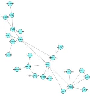
Figure (11) closes in on a region of Figure (10), a cluster of genes that is unconnected to the remaining genes in this estimate. According to Gene Ontology [see Consortium, 2000], these genes are associated with iron homeostasis. The probability that a gene has been false included in this cluster is at most 0.05.

As a second example, in Figure (12), we show a subgraph of genes associated with cellular membrane fusion. All three graphs were rendered using Cytoscape.

(22)

Figure 11: Application to Hughes dataset (closeup of Figure (10). These genes are associ-ated with iron homeostasis.

Figure 12: Application to Hughes dataset (subgraph of Figure (10). These genes are asso-ciated with cellular membrane fusion.

6.2.2 Iconix microarray data.

Next we analyzed a subset of a 10,000 gene microarray dataset from 160 drug treated rat livers Natsoulis et al. [2005]. In this study, rats were treated with a variety of fibrate, statin,

(23)

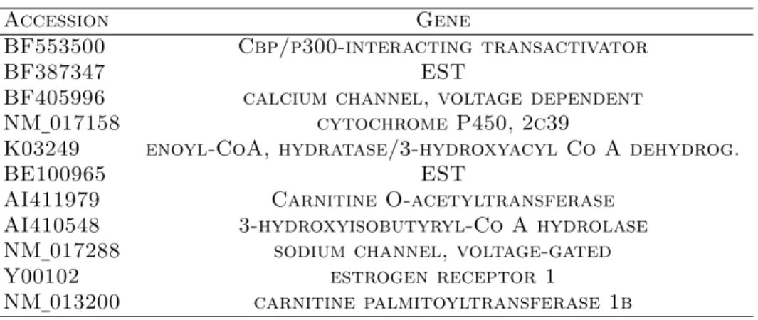
Table 1: Predictor genes for LDL receptor.

Accession Gene

BF553500 Cbp/p300-interacting transactivator

BF387347 EST

BF405996 calcium channel, voltage dependent

NM 017158 cytochrome P450, 2c39

K03249 enoyl-CoA, hydratase/3-hydroxyacyl Co A dehydrog.

BE100965 EST

AI411979 Carnitine O-acetyltransferase AI410548 3-hydroxyisobutyryl-Co A hydrolase NM 017288 sodium channel, voltage-gated

Y00102 estrogen receptor 1

NM 013200 carnitine palmitoyltransferase 1b

or estrogen receptor agonist compounds. Taking the 500 genes with the highest variance, we once again replaced α/2p2 in (3) byα, and set α= 0.05. The resulting penalty parameter isλ= 0.0853.

By applying Theorem 4 we find that all but 339 of the variables are estimated to be inde-pendent from the rest. This estimate is less conservative than that obtained in the Hughes case since the ratio of samples to variables is 160 to 500 instead of 253 to 6136.

The first order neighbors of any node in a Gaussian graphical model form the set of pre-dictors for that variable. In the estimated obtained by solving (1), we found that LDL receptor had one of the largest number of first-order neighbors in the Gaussian graphical model. The LDL receptor is believed to be one of the key mediators of the effect of both statins and estrogenic compounds on LDL cholesterol. Table 1 lists some of the first order neighbors of LDL receptor.

It is perhaps not surprising that several of these genes are directly involved in either lipid or steroid metabolism (K03249, AI411979, AI410548, NM 013200, Y00102). Other genes such as Cbp/p300 are known to be global transcriptional regulators. Finally, some are un-annotated ESTs. Their connection to the LDL receptor in this analysis may provide clues to their function.

6.2.3 Senate voting records data.

We conclude our numerical experiments by testing our approximate sparse maximum likeli-hood estimation method on binary data. The data set consists of US senate voting records data from the 109th congress (2004 - 2006). There are one hundred variables, correspond-ing to 100 senators. Each of the 542 samples is bill that was put to a vote. The votes are recorded as -1 for no and 1 for yes.

(24)

Figure 13: US Senate, 109th Congress (2004-2006). The graph displays the solution to (14) obtained using the log determinant relaxation to the log partition function of Wainwright and Jordan [2006]. Democratic senators are colored blue and Republican senators are colored red.

There are many missing values in this dataset, corresponding to missed votes. Since our analysis depends on data values taken solely from{−1,1}, it was necessary to impute values to these. For this experiment, we replaced all missing votes with noes (-1). We chose the penalty parameter λ(α) according to (19), using a significance level of α = 0.05. Figure (13) shows the resulting graphical model, rendered using Cytoscape. Red nodes correspond to Republican senators, and blue nodes correspond to Democratic senators.

We can make some tentative observations by browsing the network of senators. As neighbors most Democrats have only other Democrats and Republicans have only other Republicans. Senator Chafee (R, RI) has only democrats as his neighbors, an observation that supports media statements made by and about Chafee during those years. Senator Allen (R, VA) unites two otherwise separate groups of Republicans and also provides a connection to

(25)

Figure 14: US Senate, 109th Congress. Neighbors of Senator Allen (degree three or lower).

the large cluster of Democrats through Ben Nelson (D, NE). Senator Lieberman (D, CT) is connected to other Democrats only through Kerry (D, MA), his running mate in the 2004 presidential election. These observations also match media statements made by both pundits and politicians. Thus, although we obtained this graphical model via a relaxation of the log partition function, the resulting picture is largely supported by conventional wisdom. Figure (14) shows a subgraph consisting of neighbors of degree three or lower of Senator Allen.

Acknowledgments

We are indebted to Georges Natsoulis for his interpretation of the Iconix dataset analysis and for gathering the senate voting records. We also thank Martin Wainwright, Bin Yu, Peter Bartlett, and Michael Jordan for many enlightening conversations.

References

D. Bertsekas. Nonlinear Programming. Athena Scientific, 1998.

Gene Ontology Consortium. Gene ontology: tool for the unification of biology. Nature Genet., 25:25–29, 2000.

J. Dahl, V. Roychowdhury, and L. Vandenberghe. Covariance selection for non-chordal graphs via chordal embedding. Submitted to Optimization Methods and Software, 2006.

(26)

Alexandre d’Aspremont, Laurent El Ghaoui, M.I. Jordan, and G. R. G. Lanckriet. A direct formulation for sparse PCA using semidefinite programming. Advances in Neural Information Processing Systems, 17, 2004.

A. Dobra and M. West. Bayesian covariance selection. Working paper, ISDS, Duke Uni-versity, 2004.

J. Z. Huang, N. Liu, and M. Pourahmadi. Covariance selection and estimattion via penalized normal likelihood. Wharton Preprint, 2005.

T. R. Hughes, M. J. Marton, A. R. Jones, C. J. Roberts, R. Stoughton, C. D. Armour, H. A. Bennett, E. Coffey, H. Dai, Y. D. He, M. J. Kidd, A. M. King, M. R. Meyer, D. Slade, P. Y. Lum, S. B. Stepaniants, D. D. Shoemaker, D. Gachotte, K. Chakraburtty, J. Simon, M. Bard, and S. H. Friend. Functional discovery via a compendium of expression profiles.

Cell, 102(1):109–126, 2000.

S. Lauritzen. Graphical Models. Springer Verlag, 1996.

H. Li and J. Gui. Gradient directed regularization for sparse gaussian concentration graphs, with applications to inference of genetic networks. University of Pennsylvania Technical Report, 2005.

Z. Q. Luo and P. Tseng. On the convergence of the coordinate descent method for convex differentiable minimization. Journal of Optimization Theory and Applications, 72(1): 7–35, 1992.

N. Meinshausen and P. B¨uhlmann. High dimensional graphs and variable selection with the lasso. Annals of statistics, 34:1436–1462, 2006.

G. Natsoulis, L. El Ghaoui, G. Lanckriet, A. Tolley, F. Leroy, S. Dunlea, B. Eynon, C. Pear-son, S. Tugendreich, and K. Jarnagin. Classification of a large microarray data set: al-gorithm comparison and analysis of drug signatures. Genome Research, 15:724 –736, 2005.

Y. Nesterov. Smooth minimization of non-smooth functions. Math. Prog., 103(1):127–152, 2005.

R. Tibshirani. Regression shrinkage and selection via the lasso. Journal of the Royal statistical society, series B, 58(267-288), 1996.

Lieven Vandenberghe, Stephen Boyd, and Shao-Po Wu. Determinant maximization with linear matrix inequality constraints. SIAM Journal on Matrix Analysis and Applications, 19(4):499 – 533, 1998.

M. Wainwright and M. Jordan. Log-determinant relaxation for approximate inference in discrete markov random fields. IEEE Transactions on Signal Processing, 2006.

M. J. Wainwright, P. Ravikumar, and J. D. Lafferty. High-dimensional graphical model selection using ℓ1-regularized logistic regression. Proceedings of Advances in Neural

(27)

Appendix A. Proof of solution properties and block coordinate descent convergence

In this section, we give short proofs of the two theorems on properties of the solution to (1), as well as the convergence of the block coordinate descent method.

Proof of Theorem 1:

Since ˆΣ satisfies ˆΣ =S+ ˆU, where_kU_k∞ ≤λ, we have: kΣˆk2=kS+ ˆUk2

≤ kS_k2+kUk2 ≤ kSk2+kUk∞≤ kSk2+λp

which yields the lower bound on kΣˆ−1k2. Likewise, we can show that kΣˆ−1k2 is bounded

above. At the optimum, the primal dual gap is zero: −log det ˆΣ−1_{+ trace(}_S_Σˆ−1_{) +}_λ_k_Σˆ−1_k

1−log det ˆΣ−p = trace(SΣˆ−1) +λ_kΣˆ−1_k1−p= 0 We therefore have kΣˆ−1_k 2 ≤ kΣˆ−1kF ≤ kΣˆ−1k1 =p/λ₋trace(SΣˆ−1)/λ_≤p/λ

where the last inequality follows from trace(SΣˆ−1)≥0, sinceS0 and ˆΣ−1 ≻0.

Next we prove the convergence of block coordinate descent:

Proof of Theorem 3:

To see that optimizing over one row and column of W in (2) yields the quadratic program (4), let all but the last row and column of W be fixed. Since we know the diagonal entries of the solution, we can fix the remaining diagonal entry as well:

W = W_\p\p wp wT p Wpp

Then, using Schur complements, we have that

detW = detW\p\p·(Wpp−wTp(W\p\p)−1wp)

(28)

By general results on block coordinate descent algorithms [e.g., Bertsekas, 1998], the algo-rithms converges if and only if (4) has a unique solution at each iteration. Thus it suffices to show that, at every sweep,W(j)_≻_{0 for all columns}_j_{. Prior to the first sweep, the initial}

value of the variable is positive definite: W(0) _≻_{0 since}_W(0) _:=_S₊_λI_{, and we have}_S ₀

and λ >0 by assumption.

Now suppose thatW(j)_≻_{0. This implies that the following Schur complement is positive:} wjj−WjT(W

(j)

\j\j)

−1_W j >0

By the update rule we have that the corresponding Schur complement for W(j+1) _{is even}

greater: wjj−WjT(W (j+1) \j\j ) −1_W j > wjj−WjT(W (j) \j\j) −1_W j >0 so that W(j+1) _≻_0.

Finally, we apply Theorem 3 to prove the second property of the solution.

Proof of Theorem 4:

Suppose that column j of the second moment matrix satisfies |Sij| ≤λfor all i6=j. This

means that the zero vector is in the constraint set of (4) for that column. Each time we return to column j, the objective function will be different, but always of the form yT_Ay

forA≻0. Since the constraint set will not change, the solution for columnjwill always be zero. By Theorem 3, the block coordinate descent algorithm converges to a solution, and so therefore the solution must have ˆΣj = 0.

Appendix B. Proof of error bounds.

Next we shall show that the penalty parameter choice given in (3) yields the error probability bound of Theorem 2. The proof is nearly identical to that of [Meinshausen and B¨uhlmann, 2006,Theorem 3]. The differences stem from a different objective function, and the fact that our variable is a matrix of size p rather than a vector of size p. Our proof is only an adaptation of their proof to our problem.

B.1 Preliminaries

Before we begin, consider problem (1), for a matrixS of any size: ˆ

X= arg min−log detX+ trace(SX) +λkXk1

where we have dropped the constraintX ≻0 since it is implicit, due to the log determinant function. Since the problem is unconstrained, the solution ˆX must correspond to setting

(29)

the subgradient of the objective to zero:

Sij−Xij−1 =−λ forXij >0

Sij−Xij−1 =λ forXij <0

|Sij −Xij−1| ≤λ forXij = 0

(20)

Recall that by Theorem 1, the solution is unique for λpositive.

B.2 Proof of error bound for Gaussian data.

Now we are ready to prove Theorem 2.

Proof of Theorem 2:

Sort columns of the covariance matrix so that variables in the same connectivity component are grouped together. The correct zero pattern for the covariance matrix is then block diagonal. Define

Σcorrect := blk diag(C1, . . . , Cℓ) (21)

The inverse (Σcorrect)−1 must also be block diagonal, with possible additional zeros inside the blocks. If we constrain the solution to (1) to have this structure, then by the form of the objective, we can optimize over each block separately. For each block, the solution is characterized by (20).

Now, suppose that

λ > max

i∈N,j∈N\Ci

|Sij −Σcorrectij | (22)

Then, by the subgradient characterization of the solution noted above, and the fact that the solution is unique forλ > 0, it must be the case that ˆΣ = Σcorrect. By the definition of Σcorrect, this implies that, for ˆΣ, we have ˆCk=Ck for allk∈N.

Taking the contrapositive of this statement, we can write:

(30)

The equality at the end follows since, by definition, Σcorrect_ij = 0 forj ∈N\Ci. It remains

to boundP(|Sij| ≥λ).

The statement _|Skj| ≥λcan be written as:

|Rkj|(1−R2kj)−

1

2 ≥λ(s_kks_jj−λ2)− 1 2

whereRkj is the correlation between variablesk and j, since

|Rkj|(1−R2kj)−

1

2 =|S_kj|(S_kkS_jj −S_kj2 )− 1 2

Furthermore, the condition j _∈ N_\Ck is equivalent to saying that variables k and j are

independent: Σkj = 0. Conditional on this, the statistic

Rkj(1−Rkj2 )−

1

2(n−2) 1 2

has a Student’s t-distribution forn−2 degrees of freedom. Therefore, for all j∈N\Ck,

P(|Skj| ≥λ|Skk=skk, Sjj =sjj) = 2P(Tn−2 ≥λ(skksjj−λ2)− 1 2(n−2) 1 2|S_kk=s_kk, S_jj =s_jj) ≤2 ˜Fn−2(λ(ˆσk2σˆ2j −λ2)− 1 2(n−2)12) (24) where ˆσ2

k is the sample variance of variable k, and ˜Fn−2 = 1−Fn−2 is the CDF of the

Student’s t-distribution with n−2 degree of freedom. This implies that, for all j∈N\Ck,

P(|Skj| ≥λ)≤2 ˜Fn−2(λ(ˆσ2kˆσj2−λ2)− 1 2(n−2) 1 2) since P(A) =R P(A_|B)P(B)dB _≤ KR

P(B)dB = K. Putting the inequalities together, we have that: P(_∃k: ˆCλ k 6⊆Ck) ≤p2·maxk,j∈N\Ck2 ˜Fn−2(λ(ˆσ 2 kσˆ2j −λ2)− 1 2(n−2)12) = 2p2_F˜_n₋₂₍_λ₍₍_n₋₂₎_/_((max_i>j_σ_ˆ_k_σ_ˆ_j₎2₋_λ2₎₎1₂₎

For any fixed α, our required condition on λis therefore ˜

Fn−2(λ((n−2)/((max i>j σˆkσˆj)

2₋_λ2₎₎1

2) =α/2p2 which is satisfied by choosingλaccording to (3).

(31)

B.3 Proof of bound for binary data.

We can reuse much of the previous proof to derive a corresponding formula for the binary case.

Proof of Theorem 7:

The proof of Theorem 7 is identical to the proof of Theorem 2, except that we have a different null distribution for|Skj|. The null distribution of

nR_kj2

is chi-squared with one degree of freedom. Analogous to (24), we have:

P(|Skj| ≥λ|Skk=skk, Sjj =sjj)

= 2P(nR2_kj ≥nλ2skksjj|Skk =skk, Sjj =sjj)

≤2 ˜G(nλ2_σ_ˆ2 kσˆj2)

where ˆσ2

k is the sample variance of variablek, and ˜G= 1−Gis the CDF of the chi-squared

distribution with one degree of freedom. This implies that, for allj ∈N\Ck,

P(|Skj| ≥λ)≤2 ˜G((λσˆkσˆj√n)2)

Putting the inequalities together, we have that:

P(∃k: ˆCλ k 6⊆Ck) ≤p2_·_max k,j∈N\Ck2 ˜G((λσˆkσˆj √ n)2₎ = 2p2G˜((mini>jσˆkσˆj)2nλ2)

so that, for any fixed α, we can achieve our desired bound by choosing λ(α) according to (19).

Appendix C. Proof of connection between Gaussian SML and binary ASML

We end with a proof of Theorem 6, which connects the exact Gaussian sparse maximum likelihood problem with the approximate sparse maximum likelihood problem obtained by using the log determinant relaxation of Wainwright and Jordan [2006]. First we must prove Lemma 5.

(32)

Proof of Lemma 5:

The conjugate function for the convex normalization A(θ) is defined as

A∗(µ) := sup

θ {h

µ, θi −A(θ)} (25)

Wainwright and Jordan derive a lower bound on this conjugate function using an entropy bound:

A∗(µ)_≥B∗(µ) (26)

Since our original variables are spin variables x _{−1,+1_}, the bound given in the paper is

B∗(µ) :=₋1

2log det(R(µ) + diag(m))−

p

2log(

eπ

2 ) (27)

wherem:= (1,4₃, . . . ,4₃).

The dual of this lower bound isB(θ):

B∗₍_µ_{) := max}

θhθ, µi −B(θ)

≤maxθhθ, µi −A(θ) =:A∗(µ)

(28)

This means that, for allµ, θ,

hθ, µi −B(θ)≤A∗(µ) (29) or B(θ)_{≥ h}θ, µ_{i −}A∗(µ) (30) so that in particular B(θ)_≥max µ hθ, µi −A ∗₍_µ_{) =:}_A₍_θ₎ ₍₃₁₎

(33)

Using the definition of B(θ) and its dualB∗(µ), we can write

B(θ) := maxµhθ, µi −B∗(µ)

= p₂log(eπ₂ ) + maxµ1₂hR(θ), R(µ)i+1₂log det(R(µ) + diag(m))

= p₂log(eπ

2 ) +12 ·max{hR(θ), X−diag(m)i+ log det(X) :X ≻0,diag(X) =m}

= p₂log(eπ₂ ) +1₂ _{· {}maxX≻0minνhR(θ), X−diag(m)i+ log det(X) +νT(diag(X)−m)}

= p₂log(eπ₂ ) +1₂ · {maxX≻0minνhR(θ) + diag(ν), Xi+ log det(X)−νTm}

= p₂log(eπ

2 ) +12 · {minν−νTm+ maxX≻0hR(θ) + diag(ν), Xi+ log det(X)}

= p₂log(eπ

2 ) +12 · {minν−νTm−log det(−(R(θ) + diag(ν)))−(p+ 1)}

= p₂log(eπ₂ )−1

2(p+ 1) +12 · {minν−νTm−log det(−(R(θ) + diag(ν)))}

= p₂log(eπ

2 )−12(p+ 1)−12 · {maxννTm+ log det(−(R(θ) + diag(νλ)}

(32)

Now we use lemma 5 to prove the main result of section 5.1. Having expressed the upper bound on the log partition function as a constant minus a maximization problem will help when we formulate the sparse approximate maximum likelihood problem.

Proof of Theorem 6:

The approximate sparse maximum likelihood problem is obtained by replacing the log par-tition function A(θ) with its upper boundB(θ), as derived in lemma 5:

n_{· {}maxθ1₂hR(θ), R(¯z)i −B(θ)−λkθk1}

=n· {maxθ 1₂hR(θ), R(¯z)i −λkθk1+1₂(p+ 1)−p₂log(eπ₂)

+1₂ _{· {}maxννTm+ log det(−(R(θ) + diag(ν)))}}

= n₂(p+ 1)−np₂ log(eπ₂) +n₂ ·maxθ,ν{νTm+hR(θ), R(¯z)i

+ log det(−(R(θ) + diag(ν)))−2λkθk1}

(33)

We can collect the variables θ and ν into an unconstrained symmetric matrix variable

(34)

Observe that

hR(θ), R(¯z)_i=_h−Y ₋diag(ν), R(¯z)_i

=−hY, R(¯z)i − hdiag(ν), R(¯z)i=−hY, R(¯z)i

(34) and that