Deep Learning via Semi-Supervised Embedding
Jason Weston1, Fr´ed´eric Ratle2, Hossein Mobahi3, and Ronan Collobert4 ?? 1
Google, New York, USA.
Nuance Communications, Montreal, Canada.
3 Department of Computer Science, University of Illinois Urbana-Champaign, USA.
4 IDIAP Research Institute, Martigny, Switzerland.
Abstract. We show how nonlinear embedding algorithms popular for use with “shallow” semi-supervised learning techniques such as kernel methods can be easily applied to deep multi-layer architectures, either as a regularizer at the output layer, or on each layer of the architecture. This trick provides a simple alternative to existing approaches to deep learning whilst yielding competitive error rates compared to those methods, and existing shallow semi-supervised techniques.
Keywords: semi-supervised learning, deep learning, embedding
1
Introduction
In this chapter we describe a trick for improving the generalization ability of neural networks by utilizing unlabeled pairs of examples for semi-supervised learning. The field of semi-supervised learning (Chapelle et al., 2006) has the goal of improving generalization on supervised tasks using unlabeled data. One of the tricks they use is the so-called embedding of data into a lower dimensional space (or the related task of clustering) which are unsupervised dimensionality reduction techniques that have been intensively studied. For example, researchers have used nonlinear embedding or cluster representations as features for a su-pervised classifier, with improved results. Many of those proposed architectures are disjoint and shallow, by which we mean the unsupervised dimensionality reduction algorithm is trained on unlabeled data separately as a first step, and then its results are fed to a supervised classifier which has a shallow architec-ture such as a (kernelized) linear model. For example, several methods learn a clustering or a distance measure based on a nonlinear manifold embedding as a first step (Chapelle et al., 2003; Chapelle & Zien, 2005). Transductive Support ??
Much of the work in this chapter was completed while Jason Weston and Ronan Collobert were working at NEC labs, Princeton, USA, and while Fr´ed´eric Ratle was affiliated with the University of Lausanne, Switzerland. See (Weston et al., 2008) and (Mobahi et al., 2009) for conference papers on this subject.
Vector Machines (TSVMs) (Vapnik, 1998) (which employs a kind of clustering) and LapSVM (Belkin et al., 2006) (which employs a kind of embedding) are examples of methods that are joint in their use of unlabeled data and labeled data, while their architecture is shallow. In this work we use the same embedding trick as those researchers, but apply it to (deep) neural networks.
Deep architectures seem a natural choice in hard AI tasks which involve several sub-tasks which can be coded into the layers of the architecture. As argued by several researchers (Hinton et al., 2006; Bengio et al., 2007) semi-supervised learning is also natural in such a setting as otherwise one is not likely to ever have enough data to perform well. This is both because of the dearth of label data, and because of the difficulty of training the architectures. Secondly, intuitively one would think that training on labeled and unlabeled data
jointlyshould help guide the best use of the unlabeled data for the labeled task compared toa two-stage disjoint approach. (However, to our knowledge there is no systematic evidence of the latter).
Several authors have recently proposed methods for using unlabeled data in deep neural network-based architectures. These methods either perform a greedy layer-wise pre-training of weights using unlabeled data alone followed by super-vised fine-tuning (which can be compared to thedisjointshallow techniques for semi-supervised learning described before), or learn unsupervised encodings at multiple levels of the architecture jointly with a supervised signal. Only consid-ering the latter, the basic setup we advocate is simple:
1. Choose an unsupervised learning algorithm. 2. Choose a model with a deep architecture.
3. The unsupervised learning is plugged into any (or all) layers of the architec-ture as anauxiliary task.
4. Train supervised and unsupervised tasks using the same architecture simul-taneously.
The aim is that the unsupervised method will improve accuracy on the task at hand. In this chapter we advocate a simple way of performing deep learning by leveragingexisting ideas from semi-supervised algorithms developed in shallow
architectures. In particular, we focus on the idea of combining an embedding -based regularizer with a supervised learner to perform semi-supervised learning, such as is used in Laplacian SVMs (Belkin et al., 2006). We show that this method can be: (i) generalized to multi-layer networks and trained by stochastic gradient descent; and (ii) is valid in the deep learning framework given above. Experimentally, we also show that it seems to work quite well. We expect this is due to several effects: firstly, the extra embedding objective acts both as a data-dependent regularizer but secondly also as a weakly-supervised task that is correlated well with the supervised task of interest. Finally, adding this training objective at multiple layers of the network helps to train all the layers rather than just backpropagating from the final layer as in supervised learning.
Although the core of this chapter focuses on a particular algorithm (embed-ding) in a joint setup, we expect the approach would also work in a disjoint setup too, and with other unsupervised algorithms, for example the approach of
Transductive SVM has also been generalized to the deep learning case (Karlen et al., 2008).
2
Semi-Supervised Embedding
Our method will adapt existing semi-supervised embedding techniques for shal-low methods to neural networks. Hence, before we describe the method, let us first review existing semi-supervised approaches. A key assumption in many semi-supervised algorithms is the structure assumption5: points within the same structure (such as a cluster or a manifold) are likely to have the same label. Given this assumption, the aim is to use unlabeled data to uncover this structure. In order to do this many algorithms such as cluster kernels (Chapelle et al., 2003), LDS (Chapelle & Zien, 2005), label propagation (Zhu & Ghahramani, 2002) and LapSVM (Belkin et al., 2006), to name a few, make use of regularizers that are directly related to unsupervised embedding algorithms. To understand these methods we will first review some relevant approaches to linear and nonlinear embedding.
2.1 Embedding Algorithms
We will focus on a rather general class of embedding algorithms that can be de-scribed by the following type of optimization problem: given the datax1, . . . , xU find an embeddingf(xi) of each pointxi by minimizing
U X
i,j=1
L(f(xi, α), f(xj, α), Wij)
w.r.t. the learning paramatersα, subject to
Balancing constraint.
This type of optimization problem has the following main ingredients:
– f(x) ∈ Rn is the embedding one is trying to learn for a given example
x∈Rd. It is parametrized byα. In many techniquesf(xi) =fi is a lookup table where each exampleiis assigned an independent vector fi.
– Lis a loss function between pairs of examples.
– The matrixWof weightsWij specifies the similarity or dissimilarity between examplesxiandxj. This is supplied in advance and serves as a kind of label for the loss function.
– A balancing constraint is often required for certain objective functions so that a trivial solution is not reached.
As is usually the case for such machine learning setups, one can specify the model type (family of functions) and the loss to get different algorithmic variants. Many well known methods fit into this framework, we describe some pertinent ones below.
5
This is often referred to as the cluster assumption or the manifold assumption (Chapelle et al., 2006).
Multidimensional scaling (MDS) (Kruskal, 1964) is a classical algorithm that attempts to preserve the distance between points, whilst embedding them in a lower dimensional space, e.g. by using the loss function
L(fi, fj, Wij) = (||fi−fj|| −Wij)2
MDS is equivalent to PCA if the metric is Euclidean (Williams, 2001).
ISOMAP (Tenenbaum et al., 2000) is a nonlinear embedding technique that attempts to capture manifold structure in the original data. It works by defining a similarity metric that measures distances along the manifold, e.g.Wijis defined by the shortest path on the neighborhood graph. One then uses those distances to embed using conventional MDS.
Laplacian Eigenmaps (Belkin & Niyogi, 2003) learn manifold structure by em-phasizing the preservation of local distances. One defines the distance metric between the examples by encoding them in the Laplacian ˜L =W −D, where
Dii=PjWij is diagonal. Then, the following optimization is used: X ij L(fi, fj, Wij) = X ij Wij||fi−fj||2=f>Lf˜ (1)
subject to the balancing constraint:
f>Df =I and f>D1 = 0. (2)
Siamese Networks (Bromley et al., 1993) are also a classical method for nonlinear embedding. Neural networks researchers think of such models as a network with two identical copies of the same function, with the same weights, fed into a “distance measuring” layer to compute whether the two examples are similar or not, given labeled data. In fact, this is exactly the same as the formulation given at the beginning of this section.
Several loss functions have been proposed for siamese networks, here we describe a margin-based loss proposed by the authors of (Hadsell et al., 2006):
L(fi, fj, Wij) = (
||fi−fj||2 ifWij = 1, max(0, m− ||fi−fj||2)2 ifWij = 0
(3)
which encourages similar examples to be close, and dissimilar ones to have a distance of at least m from each other. Note that no balancing constraint is needed with such a choice of loss as the margin constraint inhibits a trivial solution. Compared to using constraints like (2) this is much easier to optimize by gradient descent.
2.2 Semi-Supervised Algorithms
Severalsemi-supervisedclassification algorithms have been proposed which take advantage of the algorithms described in the last section. Here we assume the setting where one is givenM+Uexamplesxi, but only the firstM have a known labelyi.
Label Propagation (Zhu & Ghahramani, 2002) adds a Laplacian Eigenmap type regularization to a nearest-neighbor type classifier:
min f M X i=1 ||fi−yi||2+λ M+U X i,j=1 Wij||fi−fj||2 (4)
The algorithm tries to give two examples with large weighted edgeWijthe same label. The neighbors of neighbors tend to also get the same label as each other by transitivity, hence the namelabel propagation.
LapSVM (Belkin et al., 2006) uses the Laplacian Eigenmaps type regularizer with an SVM: minimize ||w||2+γ M X i=1 H(yif(xi)) +λ M+U X i,j=1 Wij||f(xi)−f(xj)||2 (5)
whereH(x) = max(0,1−x) is the hinge loss.
Other Methods In (Chapelle & Zien, 2005) a method called graph is suggested which combines a modified version of ISOMAP with an SVM. The authors also suggest to combine modified ISOMAP with TSVMs rather than SVMs, and call itLow Density Separation(LDS).
3
Semi-supervised Embedding for Deep Learning
We would like to use the ideas developed in semi-supervised learning for deep learning. Deep learning consists of learning a model with several layers of non-linear mapping. In this chapter we will consider multi-layer networks with N
layers of hidden units that give aC-dimensional output vector:
fi(x) = d X
j=1
wO,ij hNj (x) +bO,i, i= 1, . . . , C (6)
where wO are the weights for the output layer, and typically the kth layer is defined as hki(x) =S X j wk,ij hkj−1(x) +bk,i , k >1 (7) h1i(x) =S X j w1j,i xj+b1,i (8)
andSis a non-linear squashing function such as tanh. Here, we describe a stan-dardfully connectedmulti-layer network but prior knowledge about a particular problem could lead one to other network designs. For example in sequence and image recognition time delay and convolutional networks (TDNNs and CNNs)
(LeCun et al., 1998) have been very successful. In those approaches one intro-duces layers that apply convolutions on their input which take into account locality information in the data, i.e. they learn features from image patches or windows within a sequence.
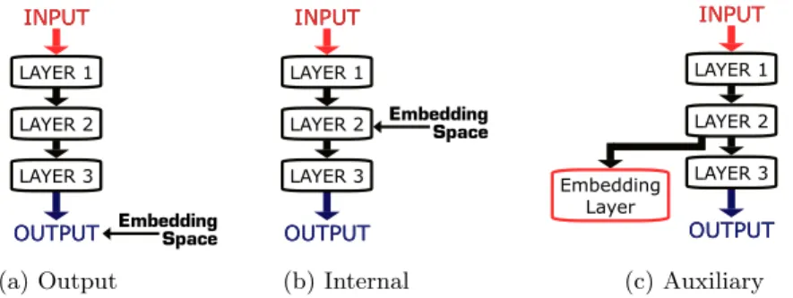
The general method we propose fordeep learning via semi-supervised embed-dingis to add a semi-supervised regularizer in deep architectures in one of three different modes, as shown in Figure 1:
(a) Add a semi-supervised loss (regularizer) to the supervised loss on the entire network’s output (6): M X i=1 `(f(xi), yi) +λ M+U X i,j=1 L(f(xi), f(xj), Wij) (9)
This is most similar to theshallowtechniques described before, e.g. equation (5).
(b) Regularize the kthhidden layer (7) directly: M X i=1 `(f(xi), yi) +λ M+U X i,j=1 L(fk(xi), fk(xj), Wij) (10) wherefk(x) = (hk
1(x), . . . , hkHUk(x)) is the output of the network up to the
kthhidden layer (HU
k is the number of hidden units on layerk).
(c) Create an auxiliary network which shares the first k layers of the original network but has a new final set of weights:
gi(x) = X j wAUX,i j h k j(x) +b AUX,i (11)
We train this network to embedunlabeled data simultaneously as we train the original network onlabeleddata.
One can use the loss function (3) for embedding, and the hinge loss
`(f(x), y) = C X
c=1
H(y(c)fc(x)),
for labeled examples, wherey(c) = 1 if y=cand -1 otherwise. For neighboring points, this is the same regularizer as used in LapSVM and Laplacian Eigenmaps. For non-neighbors, whereWij = 0, this loss “pulls” points apart, thus inhibiting trivial solutions without requiring difficult constraints such as (2). To achieve an embeddingwithoutlabeled data the latter is necessary or all examples would collapse to a single point in the embedding space. This regularizer is therefore preferable to using (1) alone. Pseudocode of the overall approach is given in Algorithm 1.
OUTPUT OUTPUT INPUT INPUT Embedding Space LAYER 1 LAYER 2 LAYER 3 OUTPUT OUTPUT INPUT INPUT LAYER 1 LAYER 2 LAYER 3 Embedding Space OUTPUT OUTPUT INPUT INPUT LAYER 1 LAYER 2 LAYER 3 Embedding Layer
(a) Output (b) Internal (c) Auxiliary Fig. 1.Three modes of embedding in deep architectures.
Algorithm 1EmbedNN
Input:labeled data (xi, yi),i= 1, . . . , M, unlabeled dataxi,i=M+ 1, . . . , U, set of functionsf(·), and embedding functionsgk(·), see Figure 1 and equations (9), (10) and (11).
repeat
Pick a randomlabeledexample (xi, yi) Make a gradient step to optimize`(f(xi), yi) foreach embedding functiongk(·)do
Pick a random pair of neighborsxi, xj. Make a gradient step forλL(gk(xi), gk(xj),1) Pick a random unlabeled examplexn. Make a gradient step forλL(gk(xi), gk(xn),0) end for
untilstopping criteria is met.
– The hyperparameter λ: in most of our experiments we simply set this to
λ= 1 and it worked well due to the alternating updates in Algorithm 1. Note however if you are using many embedding loss functions they will dominate the objective in that case.
– We note that near the end of optimization it may be advantageous to re-duce the learning rate of the regularizer more than the learning rate for the term that is minimizing the training error so that the training error can be as low as possible on noiseless tasks (however we did not try this in our experiments).
– If you use an internal embedding on the first layer of your network, it is likely that this embedding problem is harder than an internal embedding on a later layer, so you might not want to give them all the same learning rate or margin, but that complicates the hyperparameter choices. An alternative idea would be to use auxiliary layers on earlier layers, or even go through two auxiliary layers, rather than one to make the embedding task easier. Auxiliary layers are thrown away at test time.
– Embedding on the last output layer may not always be a good idea, de-pending on the type of network. For example if you are using a softmax last layer the 2-norm type embedding loss may not be appropriate for the log probability representation in the last layer. In that case we suggest to do the embedding on the last-but-one layer instead.
– Finally, although we did not try it, training in a disjoint fashion, i.e. doing the embedding training first, and then continuing training with a fine tuning step with only the labeled data, might simplify these hyperparameter choices above.
3.1 Labeling unlabeled data as neighbors (building the graph)
Training neural networks online using stochastic gradient descent is fast and can scale to millions of examples. A possible bottleneck with the described approach is computation of the matrix W, that is, computing which unlabeled examples are neighbors and have valueWij = 1. Embedding algorithms often usek-nearest neighbor for this task. Many methods for its fast computation do exist, for example hashing and tree-based methods.
However, there are also many other ways of collecting neighboring unlabeled data that do not involve computing k-nn. For example, if one has access to unlabeled sequence data the following tricks can be used:
– For image tasks one can make use of the temporal coherence of unlabeled video: two successive frames are very likely to contain similar content and represent the same concept classes. Each object in the video is also likely to be subject to small transformations, such as translation, rotation or de-formation over neighboring frames. Hence, using this with semi-supervised embedding could learn classes that are invariant to those changes. For exam-ple, one can take images from two consecutive (or close) frames of video as a neighboring pair withWij = 1. Such pairs are likely to have the same label, and are collected cheaply. Frames that are far apart are assignedWij = 0.
– For text tasks one can use documents to collect unsupervised pairs. For example, one could consider sentences (or paragraphs) of a document as neighbors that contain semantically similar information (they are probably about the same topic).
– Similarly, for speech tasks it might be possible to use audio streams in the same way.
3.2 When do we expect this approach to work?
One can see the described approach as an instance of multi-task learning (Caru-ana, 1997) using unsupervised auxiliary tasks. In common with other semi-supervised learning approaches, and indeed other deep learning approaches, given a k-nn type approach to building unlabaled pairs we only expect this to work if p(x) is useful for the supervised taskp(y|x), i.e. if the structure as-sumption is true. That is, if the decision rule lies in a region of low density with
respect to the distance metric chosen fork-nearest neighbors. We believe many natural tasks have this property.
However, if the graph is built using sequence data as described in the previous section, it is then possible that the method does not rely on the low density assumption at all. To see this, consider uniform two-dimensional data where the class label is positive if it is above the y-axis, and negative if it is below. A nearest-neighbor graph gives no information about the class label, or equivalently there is no margin to optimize for TSVMs. However, if sequence data (analogous to a video) only has data points with the same class label in consecutive frames then this would carry information. Further, no computational cost is associated with collecting video data for computing the embedding loss, in contrast to building neighbor graphs. Finally, note that in high dimensional spaces nearest neighbors might also perform poorly, e.g. in the pixel space of images.
3.3 Why is this approach good?
There are a number of reasons why the deep semi-supervised embedding trick might be useful compared to competing approaches:
– Deep embedding is very easy to optimize by gradient descent as it has a very simple loss function. This means it can be applied to any kind of neu-ral network architecture cheaply and efficiently. As well as being geneneu-rally applicable, it is also quite easy to implement.
– Compared to a reconstruction based loss function, such as used in an autoen-coder, our approach can be much cheaper to do the gradient updates. In our approach there is an encoding step, but no decoding step. That is, the loss is measured in the usually relatively low-dimensional embedding space. For high-dimensional input data (even if that data is sparse) e.g. text data, the reconstruction can be very slow, e.g. a bag-of-words representation with a dictionary of tens of thousands of words. Further, in a convolutional-pooling network architecture it might be hard to reconstruct the original data, so again an encoder-decoder system might be hard to do, but our method only requires an encoder.
– Our approach does not necessarily require the so called low density assump-tion which most other approaches depend upon. Many methods only work on data when that assumption is true (which we do not know in advance in general). Our method may still work, depending on how the pair-data is collected. This point was elaborated in the previous subsection.
4
Experimental Evaluation
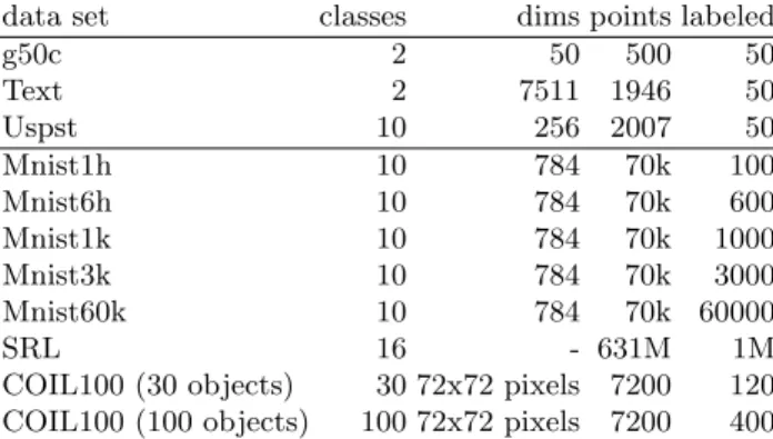
We test the semi-supervised embedding approach on several datasets summa-rized in Table 1.
Table 1. Datasets used in our experiments. The first three are small scale datasets used in the same experimental setup as found in (Chapelle & Zien, 2005; Sindhwani et al., 2005; Collobert et al., 2006). The following six datasets are large scale. The Mnist 1h, 6h, 1k, 3k and 60k variants are MNIST with a labeled subset of data, following the experimental setup in (Collobert et al., 2006). SRL is a Semantic Role Labeling task (Pradhan et al., 2004) with one million labeled training examples and 631 million unlabeled examples. COIL100 is an object detection dataset (Nene et al., 1996).
data set classes dims points labeled
g50c 2 50 500 50 Text 2 7511 1946 50 Uspst 10 256 2007 50 Mnist1h 10 784 70k 100 Mnist6h 10 784 70k 600 Mnist1k 10 784 70k 1000 Mnist3k 10 784 70k 3000 Mnist60k 10 784 70k 60000 SRL 16 - 631M 1M
COIL100 (30 objects) 30 72x72 pixels 7200 120 COIL100 (100 objects) 100 72x72 pixels 7200 400
4.1 Small-scale experiments
g50c, Text and Uspst are small-scale datasets often used for semi-supervised learning experiments (Chapelle & Zien, 2005; Sindhwani et al., 2005; Collobert et al., 2006). We followed the same experimental setup, averaging results of ten splits of 50 labeled examples where the rest of the data is unlabeled. In these experiments we test the embedding regularizer on the output of a neural network (see equation (9) and Figure 1(a)). We define a two-layer neural network (NN) with hu hidden units. We define W so that the 10 nearest neighbors of ihave
Wij = 1, andWij = 0 otherwise. We train for 50 epochs of stochastic gradient descent and fixedλ= 1, but for the first 5 we optimized the supervised target alone (without the embedding regularizer). This gives two free hyperparameters: the number of hidden units hu ={0,5,10,20,30,40,50} and the learning rate
lr={0.1,0.05,0.01,0.005,0.001,0.0005,0.0001}.
We report the optimum choices of these values optimized both by 5-fold cross validation and by optimizing on the test set in Table 2. Note the datasets are very small, so cross validation is unreliable. Several methods from the literature optimized their hyperparameters using the test set (those that are not marked with (cv)). OurEmbedNN is competitive with state-of-the-art semi-supervised methods based on SVMs, even outperforming them in some cases.
4.2 MNIST experiments
We compare our method in all three different modes (Figure 1) with conventional semi-supervised learning (TSVM) using the same data split and validation set
Table 2. Results on Small-Scale Datasets. We report the best test error over the hyperparameters of our method, EmbedNN, as in the methodology of (Chapelle & Zien, 2005) as well as the error when optimizing the parameters by cross-validation, EmbedNN(cv). LDS(cv) and LapSVM(cv) also use cross-validation.
g50c Text Uspst SVM 8.32 18.86 23.18 TSVM 5.80 5.71 17.61 LapSVM(cv) 5.4 10.4 12.7 LDS(cv) 5.4 5.1 15.8 Label propagation 17.30 11.71 21.30 Graph SVM 8.32 10.48 16.92 NN 10.62 15.74 25.13 EmbedNN 5.66 5.82 15.49 EmbedNN(cv) 6.78 6.19 15.84
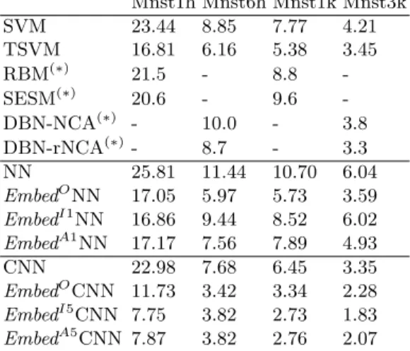
Table 3.Results on MNIST with 100, 600, 1000 and 3000 labels. A two-layer Neural Network (NN) is compared to an NN with Embedding regularizer (EmbedNN) on the output (O),ithlayer (Ii) or auxiliary embedding from theithlayer (Ai) (see Figure 1). A convolutional network (CNN) is also tested in the same way. We compare to SVMs and TSVMs. RBM, SESM, DBN-NCA and DBN-rNCA (marked with (∗)) taken from (Ranzato et al., 2007; Salakhutdinov & Hinton, 2007) are trained on a different data split. Mnst1h Mnst6h Mnst1k Mnst3k SVM 23.44 8.85 7.77 4.21 TSVM 16.81 6.16 5.38 3.45 RBM(∗) 21.5 - 8.8 -SESM(∗) 20.6 - 9.6 -DBN-NCA(∗) - 10.0 - 3.8 DBN-rNCA(∗)- 8.7 - 3.3 NN 25.81 11.44 10.70 6.04 EmbedONN 17.05 5.97 5.73 3.59 EmbedI1NN 16.86 9.44 8.52 6.02 EmbedA1NN 17.17 7.56 7.89 4.93 CNN 22.98 7.68 6.45 3.35 EmbedOCNN 11.73 3.42 3.34 2.28 EmbedI5CNN 7.75 3.82 2.73 1.83 EmbedA5CNN 7.87 3.82 2.76 2.07
Table 4.Mnist1h dataset with deep networks of 2, 6, 8, 10 and 15 layers; each hidden layer has 50 hidden units. We compare classical NN training withEmbedNN where we either learn an embedding at the output layer (O) or an auxiliary embedding on all layers at the same time (ALL).
2 4 6 8 10 15
NN 26.0 26.1 27.2 28.3 34.2 47.7
EmbedONN 19.7 15.1 15.1 15.0 13.7 11.8
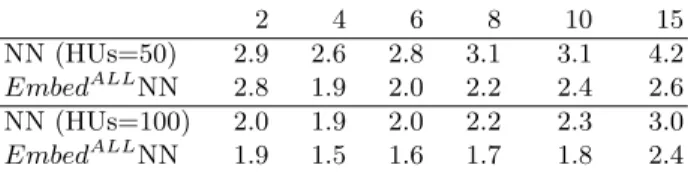
Table 5.Full Mnist60k dataset with deep networks of 2, 6, 8, 10 and 15 layers, using either 50 or 100 hidden units. We compare classical NN training withEmbedALLNN where we learn an auxiliary embedding on all layers at the same time.
2 4 6 8 10 15
NN (HUs=50) 2.9 2.6 2.8 3.1 3.1 4.2
EmbedALLNN 2.8 1.9 2.0 2.2 2.4 2.6
NN (HUs=100) 2.0 1.9 2.0 2.2 2.3 3.0
EmbedALLNN 1.9 1.5 1.6 1.7 1.8 2.4
as in (Collobert et al., 2006). We also compare to several deep learning methods: RBMs (Restricted Boltzmann Machines), SESM (Sparse Encoding Symmetric Machine), DBN-NCA and DBN-rNCA (Deep Belief Nets - (regularized) Neigh-bourhood Components Analysis). (Note, however the latter were trained on a different data split). In these experiments we consider 2-layer networks (NN) and 6-layer convolutional neural nets (CNN) for embedding. We optimize the parameters of NN (hu={50,100,150,200,400}hidden units and learning rates as before) on the validation set. The CNN architecture is fixed: 5 layers of image patch-type convolutions, followed by a linear layer of 50 hidden units, similar to (LeCun et al., 1998). The results given in Table 3 show the effectiveness of embedding in all three modes, with both NNs and CNNs.
4.3 Deeper MNIST experiments
We then conducted a similar set of experiments but with very deep architectures – up to 15 layers, where each hidden layer has 50 hidden units. Using Mnist1h, we first compare conventional NNs toEmbedALLNN where we learn an auxiliary nonlinear embedding (50 hidden units and a 10 dimensional embedding space) on each layer, as well as EmbedONN where we only embed the outputs. Re-sults are given in Table 4. When we increase the number of layers, NNs trained with conventional backpropagation overfit and yield steadily worse test error (although they are easily capable of achieving zero training error). In contrast,
EmbedALLNN improveswith increasing depth due to the semi-supervised “reg-ularization”. Embedding on all layers of the network has made deep learning
possible. EmbedONN (embedding on the outputs) also helps, but not as much. We also conducted some experiments using the full MNIST dataset, Mnist60k. Again using deep networks of up to 15 layers using either 50 or 100 hidden units
EmbedALLNN outperforms standard NN. Results are given in Table 5. Despite the lack of availability of extra unlabeled data, we still the same effect as in the semi-supervised case that NN overfits with increasing capacity, whereas Em-bedNNis more robust (even if it exhibits some overfitting compared to the opti-mal depth, it is nowhere near as pronounced.) Increasing the number of hidden units is likely to improve these results further, e.g. using 4 layers and 500 hidden units on each layer, one obtains 1.27% using EmbedALLNN. Overall, these
re-sults show that the regularization inEmbedNNALL is useful in settings outside of a semi-supervised learning.
Table 6. A deep architecture for Semantic Role Labeling with no prior knowledge outperforms state-of-the-art systems ASSERT and SENNA that incorporate knowledge about parts-of-speech and parse trees. A convolutional network (CNN) is improved by learning an auxiliary embedding (EmbedA1CNN) for words represented as 100-dimensional vectors using the entire Wikipedia website as unlabeled data.
Method Test Error
ASSERT (Pradhan et al., 2004) 16.54% SENNA (Collobert & Weston, 2007) 16.36% CNN [no prior knowledge] 18.40% EmbedA1CNN [no prior knowledge] 14.55%
4.4 Semantic Role Labeling
The goal of semantic role labeling (SRL) is, given a sentence and a relation of interest, to label each word with one of 16 tags that indicate that word’s seman-tic role with respect to the action of the relation. For example the sentence”The cat eats the fish in the pond”is labeled in the following way:”TheARG0 catARG0
eatsRELtheARG1fishARG1inARGM−LOCtheARGM−LOCpondARGM−LOC”where ARG0 and ARG1 effectively indicate the subject and object of the relation “eats” and ARGM-LOC indicates a locational modifier. The PropBank dataset includes around 1 million labeled words from the Wall Street Journal. We follow the ex-perimental setup of (Collobert & Weston, 2007) and train a 5-layer convolutional neural network for this task, where the first layer represents the input sentence words as 50-dimensional vectors. Unlike (Collobert & Weston, 2007), we do not give any prior knowledge to our classifier. In that work words were stemmed and clustered using their parts-of-speech. Our classifier is trained using only the original input words.
We attempt to improve this system by, as before, learning anauxiliary embed-dingtask. Our embedding is learnt using unlabeled sentences from the Wikipedia web site, consisting of 631 million words in total using the scheme described in Section 3. The same lookup table of word vectors as in the supervised task is used as input to an 11 word window around a given word, yielding 550 features. Then a linear layer projects these features into a 100 dimensional embedding space. All windows of text from Wikipedia are considered neighbors, and non-neighbors are constructed by replacing the middle word in a sentence window with a random word. Our lookup table indexes the most frequently used 30,000 words, and all other words are assigned index 30,001.
The results in Table 6 indicate a clear improvement when learning an auxil-iary embedding. ASSERT (Pradhan et al., 2004) is an SVM parser-based system
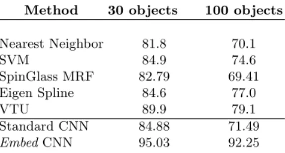
Table 7.Test Accuracy on COIL100 in various settings. Both 30 and 100 objects were used following (Wersing & K¨orner, 2003). The semi-supervised embedding algorithm using temporal coherence of video (Embed CNN) on the last but one layer of an 8 layer CNN, with various choices of video, outperforms a standard (otherwise identical) 8-layer CNN and other baselines.
Method 30 objects 100 objects Nearest Neighbor 81.8 70.1 SVM 84.9 74.6 SpinGlass MRF 82.79 69.41 Eigen Spline 84.6 77.0 VTU 89.9 79.1 Standard CNN 84.88 71.49 EmbedCNN 95.03 92.25
with many hand-coded features, and SENNA is a NN which uses part-of-speech information to build its word vectors. In contrast, our system is the only state-of-the-art method that does not use prior knowledge in the form of features derived from parts-of-speech or parse tree data. The use of neural network techniques for this application is explored in much more detail in (Collobert et al., 2011), although a different semi-supervised technique is used in that work.
4.5 Object Recognition Using Unlabeled Video
Finally, we detail some experiments using unlabeled video for semi-supervised embedding, more details of these experiments can be found in (Mobahi et al., 2009). We used the COIL100 image dataset (Nene et al., 1996) which contains color pictures of 100 objects, each 72x72 pixels. There are 72 different views for every object, i.e. there are 7200 images in total. The images were obtained by placing the objects on a turntable and taking a shot for each 5 degree turn. Note that the rotation of the objects can be viewed as an unlabeled video which we can use in our semi-supervised embedding approach.
The setup of our experiments is as follows. First, we use a standard convo-lutional neural network (CNN) without utilizing any temporal information to establish a baseline. We used an 8-layer network consisting of three sets of con-volution followed by subsampling layers, a final concon-volution layer and a fully connected layer that predicts the outputs.
For comparability with the settings available from other studies on COIL100, we choose two experimental setups. These are (i) when all 100 objects of COIL are considered in the experiment and (ii) when only 30 labeled objects out of 100 are studied (for both training and testing). In either case, 4 out of 72 views (at 0, 90, 180, and 270 degrees) per object are used for training, and the rest of the 68 views are used for testing. The results are given in Table 7 compared to some existing methods (Roobaert & Hulle, 1999; Wersing & K¨orner, 2003; Caputo et al., 2002).
To use the semi-supervised embedding trick on our CNN for video, we treat COIL100 as a continuous unlabeled video sequence of rotating objects with 72 consecutive frames per each object (after 72 frames the continuous video switches object). We perform the embedding on the last but one layer of our 8 layer CNN, i.e. on the representation yielded by the successive layers of the network just before the final softmax. For the 100 object result, the test set is hence part of the unlabeled video (a so-called “transductive” setting). Here we obtained 92.25% accuracy (EmbedCNN) which is much higher than the best alternative method (VTU) and the standard CNN that we trained.
A natural question is what happens if we do not have access to test data during training, i.e. the setting is a typical semi-supervised situation rather than a “transductive” setting. To explore this, we used 30 objects as the primary task, i.e. 4 views of each object in this set were used for training, and the rest for test. The other 70 objects only were treated as an unlabeled video sequence (again, images of each object were put in consecutive frames of a video sequence). Training with 4 views of 30 objects (labeled data) and 72 views of 70 objects (unlabeled video sequence) resulted in an accuracy of 95.03% on recognizing 68 views of the 30 objects. This is about 10% above the standard CNN performance.
5
Conclusion
In this chapter, we showed how one can improve supervised learning for deep architectures if one jointly learns an embedding task using unlabeled data. Re-searchers using shallowarchitectures already showed two ways of using embed-ding to improve generalization: (i) embedembed-ding unlabeled data as aseparate pre-processing step (i.e., first layer training) and; (ii) using embedding as a regular-izer (i.e., at the output layer). It appears similar techniques can also be used for multi-layer neural networks as well, using the tricks described in this chapter.
Bibliography
Belkin, M., & Niyogi, P. (2003). Laplacian eigenmaps for dimensionality reduction and data representation. Neural Computation,15, 1373–1396.
Belkin, M., Niyogi, P., & Sindhwani, V. (2006). Manifold regularization: a geometric framework for learning from Labeled and Unlabeled Examples. Journal of Machine Learning Research,7, 2399–2434.
Bengio, Y., Lamblin, P., Popovici, D., & Larochelle, H. (2007). Greedy layer-wise training of deep networks. Advances in Neural Information Processing Systems, NIPS 19.
Bromley, J., Bentz, J. W., Bottou, L., Guyon, I., LeCun, Y., Moore, C., Sackinger, E., & Shah, R. (1993). Signature verification using a siamese time delay neural network. International Journal of Pattern Recognition and Artificial Intelligence,7.
Caputo, B., Hornegger, J., Paulus, D., & Niemann, H. (2002). A spin-glass markov random field for 3-d object recognition(Technical Report LME-TR-2002-01). Institut fur Informatik, Universitat Erlangen Nurnberg.
Caruana, R. (1997). Multitask Learning. Machine Learning,28, 41–75.
Chapelle, O., Sch¨olkopf, B., & Zien, A. (2006). Semi-supervised learning. Adaptive computation and machine learning. Cambridge, Mass., USA: MIT Press.
Chapelle, O., Weston, J., & Sch¨olkopf, B. (2003). Cluster kernels for semi-supervised learning. NIPS 15(pp. 585–592). Cambridge, MA, USA: MIT Press.
Chapelle, O., & Zien, A. (2005). Semi-supervised classification by low density separa-tion. International Conference on Artificial Intelligence and Statistics (AISTATS) (pp. 57–64).
Collobert, R., Sinz, F., Weston, J., & Bottou, L. (2006). Large scale transductive svms. Journal of Machine Learning Research,7, 1687–1712.
Collobert, R., & Weston, J. (2007). Fast semantic extraction using a novel neural network architecture. Proceedings of the 45th Annual Meeting of the Association of Computational Linguistics, 25–32.
Collobert, R., Weston, J., Bottou, L., Karlen, M., Kavukcuoglu, K., & Kuksa, P. (2011). Natural language processing (almost) from scratch.The Journal of Machine Learn-ing Research,12, 2493–2537.
Hadsell, R., Chopra, S., & LeCun, Y. (2006). Dimensionality reduction by learning an invariant mapping. Proc. Computer Vision and Pattern Recognition Conference (CVPR’06). IEEE Press.
Hinton, G. E., Osindero, S., & Teh, Y.-W. (2006). A fast learning algorithm for deep belief nets. Neural Comp.,18, 1527–1554.
Karlen, M., Weston, J., Erkan, A., & Collobert, R. (2008). Large scale manifold trans-duction. Proceedings of the 25th international conference on Machine learning(pp. 448–455).
Kruskal, J. (1964). Multidimensional scaling by optimizing goodness of fit to a non-metric hypothesis. Psychometrika,29, 1–27.
LeCun, Y., Bottou, L., Bengio, Y., & Haffner, P. (1998). Gradient-based learning applied to document recognition. Proceedings of the IEEE,86.
Mobahi, H., Collobert, R., & Weston, J. (2009). Deep learning from temporal coher-ence in video. Proceedings of the 26th Annual International Conference on Machine Learning(pp. 737–744).
Nene, S., Nayar, S., & Murase, H. (1996). Columbia object image library (coil-100). Technical Report CUCS-006-96, February 1996.
Pradhan, S., Ward, W., Hacioglu, K., Martin, J., & Jurafsky, D. (2004). Shallow semantic parsing using support vector machines.Proceedings of HLT/NAACL-2004. Ranzato, M., Huang, F., Boureau, Y., & LeCun, Y. (2007). Unsupervised learning of invariant feature hierarchies with applications to object recognition.Proc. Computer Vision and Pattern Recognition Conference (CVPR’07). IEEE Press.
Roobaert, D., & Hulle, M. M. V. (1999). View-based 3d object recognition with support vector machines. In IEEE International Workshop on Neural Networks for Signal Processing(pp. 77–84).
Salakhutdinov, R., & Hinton, G. (2007). Learning a Nonlinear Embedding by Preserv-ing Class Neighbourhood Structure. International Conference on Artificial Intelli-gence and Statistics (AISTATS).
Sindhwani, V., Niyogi, P., & Belkin, M. (2005). Beyond the point cloud: from trans-ductive to semi-supervised learning.International Conference on Machine Learning, ICML.
Tenenbaum, J., de Silva, V., & Langford, J. (2000). A global geometric framework for nonlinear dimensionality reduction. Science,290, 2319–2323.
Vapnik, V. N. (1998). Statistical learning theory. John Wiley and Sons, New York. Wersing, H., & K¨orner, E. (2003). Learning optimized features for hierarchical models
of invariant recognition. Neural Computation,15, 1559–1599.
Weston, J., Ratle, F., & Collobert, R. (2008). Deep learning via semi-supervised em-bedding. Proceedings of the 25th international conference on Machine learning(pp. 1168–1175).
Williams, C. (2001). On a connection between kernel PCA and metric multidimensional scaling. Advances in Neural Information Processing Systems, NIPS 13.
Zhu, X., & Ghahramani, Z. (2002). Learning from labeled and unlabeled data with label propagation(Technical Report CMU-CALD-02-107). Carnegie Mellon University.