Louisiana State University
LSU Digital Commons
LSU Doctoral Dissertations
Graduate School
June 2019
High-Performance Computing Frameworks for
Large-Scale Genome Assembly
Sayan Goswami
Louisiana State University and Agricultural and Mechanical College, [email protected]
Follow this and additional works at:
https://digitalcommons.lsu.edu/gradschool_dissertations
Part of the
Bioinformatics Commons,
Computational Biology Commons,
Genomics Commons,
Other Computer Sciences Commons, and the
Software Engineering Commons
This Dissertation is brought to you for free and open access by the Graduate School at LSU Digital Commons. It has been accepted for inclusion in LSU Doctoral Dissertations by an authorized graduate school editor of LSU Digital Commons. For more information, please [email protected].
Recommended Citation
Goswami, Sayan, "High-Performance Computing Frameworks for Large-Scale Genome Assembly" (2019).LSU Doctoral Dissertations. 4942.
HIGH-PERFORMANCE COMPUTING FRAMEWORKS FOR
LARGE-SCALE GENOME ASSEMBLY
A Dissertation
Submitted to the Graduate Faculty of the Louisiana State University and Agricultural and Mechanical College
in partial fulfillment of the requirements for the degree of
Doctor of Philosophy in
The Department of Computer Science
by Sayan Goswami
B.Tech, National Institute of Technology Durgapur, India, 2011 August 2019
Acknowledgments
This work would not have been possible without the guidance, encouragement, support, and criticism of my advisors Dr. Kisung Lee and Dr. Seung-Jong Park. I would like to express my most sincere gratitude to my committee members Dr. Jianhua Chen and Dr. Richard Ng for contributing their valuable time for me. I am also grateful to my colleagues and coauthors Arghya, Shayan, and Richard, whom I had the great pleasure of working with.
I attribute my success to the unwavering support and faith of my parents, my aunt, and my brother. Thanks also to Dr. Guhathakurta (Parag Da) of NIT Durgapur who played a de-cisive role in my return to grad school. I am also deeply indebted (somewhat literally) to my friends here at Baton Rouge who have made this place my home. Many thanks to Arnab, Sujana, Saikat, Ishita, Trina, Ananya, and my past and present flatmates Arghya, Subhajit, Sa-tadru, and Joy. Lastly, a special note of gratitude must be set aside for my friends back home (Abhishek, Ayan, Gourav, JD, Sandeep, Saradendu, Saubhik, Souvik, Subh, Suprakash) with whom I spent the best years of my life.
The works presented here were partially funded by NIH grants (P20GM103458-10, P30GM-110760-03, and P20GM103424), NSF grants (MRI-1338051, IBSS-L-1620451, SCC-1737557, and RAPID-1762600), LA Board of Regents grants (LEQSF(2016-19)-RD-A-08 and ITRS), and IBM faculty awards. I would also like to thank NVIDIA for its generosity in allowing me to use their computing resources.
Table of Contents
ACKNOWLEDGMENTS . . . iii LIST OF TABLES . . . v LIST OF FIGURES . . . vi ABSTRACT . . . vii CHAPTER 1. THE GENOME ASSEMBLY PROBLEM . . . 11.1. Introduction . . . 1
1.2. De Novo Assembly - de Bruijn vs String Graphs . . . 2
1.3. Our Contribution . . . 5
2. MEMORY-EFFICIENT DISTRIBUTED DE BRUIJN GRAPH ASSEMBLY . . . 7
2.1. Introduction . . . 7 2.2. Related Work . . . 8 2.3. Methodology . . . 9 2.4. Implementation . . . 14 2.5. Evaluation . . . 23 2.6. Conclusion . . . 26
3. GPU-ACCELERATED STRING GRAPH ASSEMBLY . . . 28
3.1. Introduction . . . 28
3.2. Related Work . . . 30
3.3. Methodology for GPU-Accelerated Assembly . . . 31
3.4. Evaluation . . . 44
3.5. Conclusion . . . 50
4. THIRD GENERATION SEQUENCING & FUTURE WORK . . . 53
4.1. Third Generation Sequencing . . . 53
4.2. Advantages and Challenges of 3GS . . . 54
4.3. Background and Related Work . . . 56
4.4. Methodology . . . 59
4.5. Evaluation . . . 68
4.6. Conclusion . . . 71
APPENDIX. COPYRIGHT INFORMATION . . . 72
REFERENCES . . . 75
List of Tables
3.1. Illumina datasets used for evaluation . . . 44
3.2. Single node assembly times on 128 GB host memory and 12 GB de-vice memory (K40) . . . 46
3.3. Single node assembly times on 64 GB host memory and 6 GB device memory (K20) . . . 46
3.4. Peak memory usage (in GB) on 128 GB host with K40 . . . 47
3.5. Peak memory usage (in GB) on 64 GB host with K20 . . . 47
3.6. Comparison between SGA and LaSAGNA . . . 48
4.1. Overview of datasets . . . 69
4.2. Comparison of assembly times . . . 71
List of Figures
1.1. Overview of genome sequencing . . . 2
1.2. Overview of de Bruijn graph based assembly . . . 4
1.3. String graph-based assembly . . . 5
2.1. Classification of assemblers wrt. scalability and memory efficiency . . . 8
2.2. Partitioning de Bruijn graphs using minimum substrings. . . 11
2.3. Imbalance of distribution in intermediate data among partitions . . . 13
2.4. System overview of Lazer . . . 15
2.5. Actor interactions during map-phase . . . 16
2.6. Actor interactions during reduce-phase . . . 19
2.7. Execution times of Lazer on the synthetic wheat W7984 dataset (1.1 TB) . . . 24
2.8. Execution times of Lazer, Swap, and Ray on the Yoruban male dataset (452 GB) . . . 25
2.9. Distribution of intermediate key-value pairs with various cluster configurations . . . 27
3.1. Conceptual view of memory types . . . 31
3.2. Overview of assembly pipeline . . . 33
3.3. The communication and computing patterns while generating prefix fingerprints ofGATACCAGTAwith radix 4 and prime 13. . . 34
3.4. The communication and computing patterns while generating suffix fingerprints using prefix fingerprints . . . 35
3.5. Generating contigs from paths in string graph . . . 42
3.6. Effects of different host and device block-sizes . . . 49
3.7. Effects of different GPUs and host block-sizes . . . 49
3.8. Execution times on different node configurations . . . 51
4.1. Erroneous assembly due to repeats . . . 54
Abstract
Genome sequencing technology has witnessed tremendous progress in terms of through-put and cost per base pair, resulting in an explosion in the size of data. Typical de Bruijn graph-based assembly tools demand a lot of processing power and memory and cannot as-semble big datasets unless running on a scaled-up server with terabytes of RAMs or scaled-out cluster with several dozens of nodes.
In the first part of this work, we present a distributed next-generation sequence (NGS) assembler called Lazer, that achieves both scalability and memory efficiency by using par-titioned de Bruijn graphs. By enhancing the memory-to-disk swapping and reducing the network communication in the cluster, we can assemble large sequences such as human genomes (~400 GB) on just two nodes in 14.5 hours, and also scale up to 128 nodes in 23 minutes. We also assemble a synthetic wheat genome with 1.1 TB of raw reads on 8 nodes in 18.5 hours and on 128 nodes in 1.25 hours.
In the second part, we present a new distributed GPU-accelerated NGS assembler called LaSAGNA, which can assemble large-scale sequence datasets using a single GPU by build-ing strbuild-ing graphs from approximate all-pair overlaps in quasi-linear time. To use the limited memory on GPUs efficiently, LaSAGNA uses a two-level semi-streaming approach from disk through host memory to device memory with restricted access patterns on both disk and host memory. Using LaSAGNA, we can assemble the human genome dataset on a single NVIDIA K40 GPU in 17 hours, and in a little over 5 hours on an 8-node cluster of NVIDIA K20s.
In the third part, we present the first distributed 3rd generation sequence (3GS) assembler which uses a map-reduce computing paradigm and a distributed hash-map, both built on a high-performance networking middleware. Using this assembler, we assembled an Oxford Nanopore human genome dataset (~150 GB) in just over half an hour using 128 nodes whereas existing 3GS assemblers could not assemble it because of memory and/or time limitations.
Chapter 1. The Genome Assembly Problem
1.1. Introduction
Thegenome of an organism is composed of its entire set of DNA including all its genes, and the study of its structure, function, evolution and mapping is known asGenomics. Accord-ing to a report released in 2013, the field of genomics has contributed nearly US$1 trillion to the US economy since the start of the Human Genome Project [25]. Since a genome encodes enough information to construct entire organisms, and thus potentially has clues to treat, cure, or prevent various diseases, the knowledge of DNA sequences is being widely used not only in basic biological sciences but also in various applied fields such as medicine, forensic science, and virology [2, 30, 51].
Obtaining an organism’s DNA information consists of two essential steps - DNA sequenc-ing and sequence assembly.Sequencing is the process of chemically marking the nucleotides in order to find their exact order in the DNA. Since state-of-the-art sequencing machines can-not accurately sequence the entire genome in one go, they apply a method known asshotgun sequencing in which they create thousands of clones from the original genome, split them at random positions generating millions of smaller fragments, and sequence these to pro-duceshort-reads. Figure 1.1 depicts the process of cloning and extracting short reads from a genome.
The idea behind this type of sequencing is that each clone contributes one or more frag-ments from quasi-random locations within itself, and thus there is a high probability that fragments from different clones will have an overlap between them. The overlap information is then used to align and merge the short-reads to recreate the original sequence. This process is known asgenome assembly.
Genome assembly can be performed either by mapping or de novo. Inmapping assem-bly, reads are aligned with some reference genome of the same or a closely related species and the aligned reads are used to construct the original sequence. On the other hand, inde novo
(a) Original sequence
(b) Clones of original sequence
(c) Short-reads extracted from clones
Figure 1.1. Overview of genome sequencing
often while sequencing a new species, de novo assembly is the only option available to prac-titioners. In this work we only focus on de novo assembly since it is more compute-intensive and data-intensive than mapping assembly.
1.2. De Novo Assembly - de Bruijn vs String Graphs
In its simplest form, de novo assembly can be viewed as solving the shortest common superstring problem which takes a setRof strings {r1,r2,r3,···,rn}, and attempts to find the
shortest possible stringssuch that everyri∈Ris a substring ofs. However, the shortest
com-mon superstring problem is NP-complete and therefore all approaches to de novo assembly are heuristics that try to find suboptimal solutions in a reasonable amount of time. The main challenge in the assembly is to create a full-text index using all reads so that the overlaps be-tween them can be obtained efficiently, and subsequently storing this overlap information in a graph so that overlapping reads can be merged to generate an approximation ofs.
The method used to find overlaps between short-reads in most assemblers falls into one of two categories - de Bruijn graph based and string graph based. In the former, short-reads are further broken down into smaller overlapping sub-sequences of lengthk, calledk-mers, using a sliding window of sizek. Thesek-mers are then used to build a de Bruijn graph using the following rules:
1. Each uniquek-mer is represented as a vertex in the graph. If the samek-mer is gener-ated more than once from one or more short reads, they must be mapped to the same vertex.
2. An edge exists between two verticesvi andvj if their correspondingk-mers,ki andkj,
have an overlap ofk−1 characters between them. In other words, if thek−1 suffix ofki
is equal to thek−1 prefix ofkj, then there must be an edge fromvitovjin the generated
De Bruijn graph.
Using this technique, short-reads are represented as paths in the graph and overlaps (of length
k or longer) between reads are encoded in the graph due to the fact that samek-mers from different reads are mapped to the same vertex.
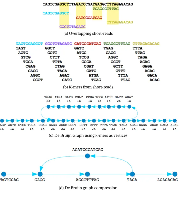
The next phase in this type of assembly is a lossless compression of each vertex chain (i.e., a path of vertices with one in-degree and one out-degree) into a single vertex calledcontig, which represents a longer substring of the original DNA sequence. The compression can be performed by traversing the graph starting from the vertices having an unequal in-degree and out-degree (such as forks, joins, etc). Each contig will contain the original sub-sequence(s) from which the participatingk-mers were produced. The compressed graph can then be used in a wide variety of contig extension strategies. Figure 1.2 presents an example of the pro-cess described above. Figure 1.2a shows a set of overlapping short reads covering the genome followed by figure 1.2b which depicts the generation of4-mers from short reads. Next, in fig-ure 1.2c, we create a de Bruijn graph using the 4-mers from the previous step. The numbers below thek-mers denote their corresponding frequencies across all reads. Note thatk-mer
TAGAappears in both the second and the fifth short reads. In the second read, thek-mer fol-lowingTAGAisAGAT, whereas in the fifth read, the following one isAGAG.Therefore, the vertex
TAGAhas two outgoing edges to verticesAGATandAGAG. Finally, in figure 1.2d we compress all unambiguous paths (chains of vertices) into contigs.
One of the disadvantages of the de Bruijn graph based assembly technique is that it is prone to collapsing repeated regions of the genome that are larger thank, causing
informa-(a) Overlapping short-reads
(b) K-mers from short-reads
(c) De Bruijn Graph using k-mers as vertices
(d) De Bruijn graph compression
Figure 1.2. Overview of de Bruijn graph based assembly
tion loss [27]. This can be avoided if assembly is performed using string-graphs which take a more direct approach in finding the overlaps between short-reads. Given a setR of reads and their Watson Crick (WC) complements, a string graphG in its simplest form consists of
R as vertices and a set of directed weighted edges E. An edgee =(ri,rj,l), whereri,rj ∈R
rj. Naturally, any edgee=(ri,rj,l)∈E must also have a complementary edgee′ =(rj′,ri′,l),
whereri′is the WC-complement ofri.
In theory, there exists a tour inG that corresponds to the original sequence from which
Rwas generated. However, the graph contains a lot of redundant information in the form of transitive edges. Specifically, if a readrj overlaps withrkand readrioverlaps with bothrjand
rk, then the edge (ri,rk) can be removed fromGwithout any information loss. Furthermore, a
read that is completely contained in another one may also be removed. A heuristic that is often used to prune the graph is a greedy approach, where only one outgoing edge corresponding to the read with the longest overlap is considered for assembly, and the others are ignored [18, 28].
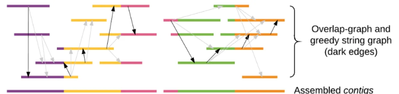
Once the graph is simplified, paths that can be unambiguously traversed are spelled out to obtain contigs. Fig. 1.3 shows a string graph created from short reads and the contigs gener-ated by traversing it. The darker lines represent the greedy edges cregener-ated between reads with the longest overlap.
Figure 1.3. String graph-based assembly
1.3. Our Contribution
The last decade has witnessed huge leaps in the advancement of sequencing technology that has led to the development of second generation sequencers, also known as Next Gener-ation sequencers (NGS), which produce sequence datasets at a much higher throughput and at a much lower cost than their predecessors. For instance, in a single run, an Illumina HiSeq 4000 sequencer can generate up to five billion 150-nucleotide reads at a cost of about $0.05 per million bases. This phenomenon has resulted in an explosion of raw datasets both in
terms of size and quantity. Although several tools have been developed to process these high-throughput sequence datasets, assembling a real-world human genome dataset whose size is nearly half a terabyte still requires either a up machine with terabytes of RAM or a scale-out cluster with several dozens of nodes. Even with the pay-as-you-go pricing model of cloud services and availability of various big data frameworks, access to such high-end machines or large-scale clusters is often too expensive for most researchers.
When processing large genomic datasets, both the de Bruijn graph and the string graph based approaches require lots of memory as well as compute power. Our common objective in the following works is to find new ways to reduce the memory requirements of the assembly process as well as its execution time. To that end, we propose two new assembly frameworks called Lazer and LaSAGNA, that are capable of processing large-scale sequence datasets using modest computing resources in a reasonable amount of time. Lazer is a fully distributed de Bruijn graph-based assembler than can assemble the human genome on two nodes with 64 GB memory each, but can scale up all the way to 128 nodes, and to the best of our knowledge, is the only distributed assembler to be able to do so. On the other hand, LaSAGNA is a string graph based assembler that is capable of assembling the large datasets on a single GPU but can also speed up the process by using multiple GPUs across a high-performance computing cluster. To the best of our knowledge, LaSAGNA is the only GPU-based assembler than can assemble a 400 GB human genome dataset on a single GPU with 6 GB device memory.
The rest of the literature is organized as follows. In Chapter 2, we explain some of the the issues with de Bruijn graph based de novo assembly, specially with respect to memory re-quirement and scalability and demonstrate how Lazer alleviates them by swapping in and out graph partitions from disk to memory. In Chapter 3, we focus on string graph based assembly and propose a semi-streaming approach to utilize the high computational capabilities of gen-eral purpose GPUs to assemble large datasets despite the limited device-memories. Finally, in Chapter 4, we provide a preliminary exposition on third generation sequencers, their advan-tages, challenges and opportunities and use them to motivate our proposed future work.
Chapter 2. Memory-Efficient Distributed De Bruijn Graph Assembly
2.1. Introduction
When it comes to de Bruijn graph based assembly, most of the widely used distributed assemblers are designed with the assumption that users will have enough resources to deal with all sizes of data. However, this is not always the scenario, particularly in case of terabyte-scale datasets where these tools run out of memory on small clusters. Furthermore, the trends in sequencing technology shows an increasing demand for processing power and memory in order for the sequences to be assembled. Consequently, researchers will soon be unable to assemble the larger genomes on the HPC clusters available to them. Therefore, to keep in-tune with the decreasing cost of sequencing, there is a need for assembly tools to be more memory efficient.
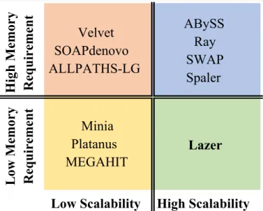
Figure 2.1 categorizes representative assemblers based on memory utilization and scal-ability. On one hand, we have the first generation assemblers which are multithreaded ap-plications that run on a single node but require terabytes of memory to assemble the larger genomes. On the other hand, we have distributed assemblers that still need huge amounts memory, but can be run on a distributed environment if there isn’t enough memory on a single node. At the other end of the spectrum, there are a few assemblers that use succinct data struc-tures to assemble large genomes on single nodes, but are not designed to run on distributed systems. In this chapter, we presentLazer(large-scale genome assembly on ZeroMQ), a dis-tributed assembly tool designed to have a low memory footprint and yet is capable of scaling up to hundreds of nodes.
Experiments on a human genome dataset (452 GB) demonstrate that Lazer’s performance is often better than others in terms of execution times, while having better scalability with a much smaller memory requirement. Moreover, Lazer successfully assembles a 1.1 TB syn-thetic wheat dataset whereas the other assemblers have failed to execute on it.
This chapter was previously published by Sayan Goswami et.al. as "Lazer: Distributed memory-efficient assembly of large-scale genomes" in 2016 IEEE International Conference on Big Data (Big Data). Reprinted by permission of IEEE.
H
igh
M
emor
y
R
eq
u
ir
eme
n
t
Velvet
SOAPdenovo
ALLPATHS-LG
ABySS
Ray
SWAP
Spaler
Low
M
emor
y
R
eq
u
ir
eme
n
t
Minia
Platanus
MEGAHIT
Lazer
Low Scalability
High Scalability
Figure 2.1. Classification of assemblers wrt. scalability and memory efficiency
The rest of the chapter is organized as follows. In Section 2.2, we discuss the current state of the art in the realm of distributed assemblers. In Sections 2.3 and 2.4, we explain the methodology and implementation details of our proposed assembler. Section 2.5 evalu-ates our tool on a variety of datasets and cluster configurations followed by a conclusion of our study in Section 2.6.
2.2. Related Work
De novo assembly is a widely studied problem so there are many assembly tools to choose from. The computation of older assemblers such as Velvet [62], ALLPATHS-LG [45], SOAP-denovo [61], etc. are restricted to a single node, and hence these tools cannot address the challenges involved in next-generation sequencing data. Furthermore, these assemblers are severely limited due to inefficient memory management and are incapable of assembling ter-abytes of data in most practical cases.
To reduce the memory required to assemble large datasets, Minia [15], Platanus [29], MegaHit [36] make use of several succinct data structures (e.g., Bloom filter, etc.) and en-coding schemes. However, their execution times are limited by the number of cores available in a single machine. Moreover, given the trends of NGS dataset sizes, it is not clear if these
as-semblers will be able to accommodate the de Bruijn graphs in the memory of a single machine in the future. Hence, a distributed approach is necessary to alleviate the problems involved in large scale NGS dataset.
Assemblathon2 [11] evaluates several de novo assemblers using a variety of datasets. The only distributed assemblers evaluated in Assemblathon2 are ABySS [56] and Ray [8], both of which are based on MPI (Message Passing Interface). We have experimentally observed that on large datasets, Ray could not scale up, and ABySS was unable to run at all. PASHA [41] is another distributed assembler, also based on MPI but is severely constrained due to that fact that some of its stages are not distributed. SWAP [47] outperforms ABySS, Ray, and PASHA both in terms of scalability as well as execution time, but has a large memory overhead.
To tackle the scalability problem, assembly tools based on Apache Hadoop or Apache Spark have also been proposed. Contrail [54] was the first de Bruijn graph-based assembler built on Hadoop, followed by CloudBrush [13], which was based on string graphs. However, in case of extremely large datasets their performances deteriorate due the disk-based computa-tion (i.e., huge amount of disk I/O is required) of Hadoop. Some assemblers such as GiGA [32] used a hybrid approach by using Hadoop for building the graph and Apache Giraph for com-pressing it. Other developments include Spaler [1], which is a de novo assembler built on Spark and GraphX. Although Spaler appears to perform well on datasets up to 100 GB, we could not access its code to evaluate it on the terabyte-scale datasets.
2.3. Methodology
Our tool comprises of the first two phases of the assembly pipeline - de Bruijn graph cre-ation and compression. In principle, the graph can be created simply by loading thek-mers into an in-memory hash map, thus implicitly merging uniquek-mers to the same vertex. A more memory-efficient option would have been to use a map-reduce-based approach where key-value pairs are partitioned into buckets and then each bucket is reduced by sorting or in-dexing the keys. However, regardless of the method used to build the graph, it must reside in an in-memory hash table in order to be traversed.
This approach poses a few significant challenges. Firstly, either there must be an enor-mous amount of memory in a single machine, or the hash map must be distributed. Secondly, in case the hash map is distributed, the lookup time is dominated by the network latency, which is generally in the order of microseconds as opposed to the nanosecond latencies of main memory. This network latency has a significant impact on the total execution time.
We alleviate the problems of scalability and memory efficiency to some extent by parti-tioning the de Bruijn graph. Our partitioned graph has two advantages:
• It does not require the entire graph to be loaded in memory at once. The vertices within each partition can be indexed, locally compressed, and spilled onto disk until all parti-tions are processed. Finally, all partiparti-tions can be loaded at once and compressed one last time.
• Each partition can be compressed by a thread or a group of threads within a single node in the cluster. This local processing reduces the necessity of synchronization and com-munication between threads and cluster nodes, thus enhancing the degree of paral-lelism.
We use minimum substring partitioning (MSP) [38] to distribute thek-mers among the different buckets. In this scheme, a smaller window of size m is slid over eachk-merKi to
generate a setSi ofk−m+1 substrings. Since|Σ| =4, each substring inSi can be uniquely
mapped to one of 4m partitions. The partition to whichKi would be mapped is determined
by the alphabetically smallest substring in Si. The motivation behind using this approach
instead of an ordinary hash function is that overlappingk-mers (where the prefix of one is the suffix of the another), which will be close to each other in the final de Bruijn graph, will have a better chance of being mapped to the same bucket. In addition, this heuristic allows us to partition the graph while it is being generated from the reads. Therefore, we can reap the obvious benefits of working with smaller sub-graphs without having a separate partitioning phase in the assembly pipeline.
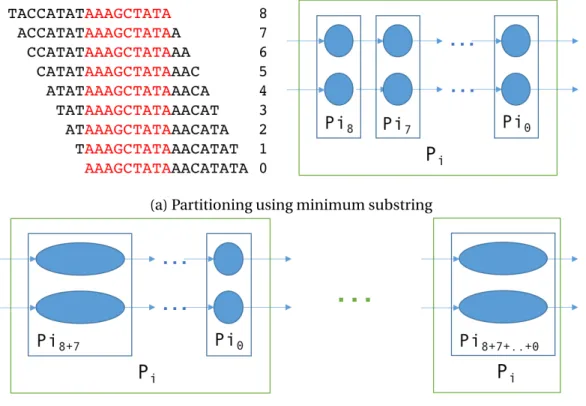
In order to reduce the memory footprint even further, we propose a two-level partitioning scheme. The first level (L1) partition of a k-mer is determined by the minimum substring as explained earlier. The second level (L2) is determined by the position of the minimum substring in thek-mer. Thus, for each L1 partition, there arek−m+1 L2 partitions. With this scheme, whenever an L1 partition is locally compressed, at most two consecutive L2 partitions are required to be loaded in memory at once, and the compression proceeds in a lockstep fashion. Figure 2.2a depicts the partitioning scheme described above and 2.2b shows the local compression of L1 partitionPi. In this example, thek-mer size is 17 and the substring size is
9. All the overlappingk-mers here have the same minimum substring (AAAGCTATA) and are
(a) Partitioning using minimum substring
(b) Local compression of partitions
Figure 2.2. Partitioning de Bruijn graphs using minimum substrings
thus mapped to the same L1 partition. However in each of thek-mers, the substring occurs at different positions and are hence mapped to different L2 partitions. The compression begins with the vertices in L2 partition Pi8 as seeds. The vertices inPi7 are loaded in a hash map,
partitionsPi7 throughPi0are merged with those inPi8. We describe our proposed techniques
for the two phases in more detail as follows. 2.3.1. De Bruijn graph creation
Map phase. In this phase, each mapper thread reads the sequences of nucleotides from files assigned to it. For each sequence of lengthl, a mapper slides a window of sizek to generate
l−k intermediate key-value pairs. A key is a byte-encoded k-mer, and the value is a tuple consisting of the two nucleotides at the either end of the window. We call them "intermedi-ate" because multiple short reads may generate the same key whose values must be merged to obtain a final key-value pair. Conceptually, each key represents a vertex of the de Bruijn graph, and its intermediate value represents at most one incoming edge and at most one out-going edge.K-mers at the leftmost and rightmost end of the sequence are padded with special characters in the value tuple to represent no incoming and outgoing edges respectively. Each key-value pair is then placed into the appropriate partition based on the minimum substring of the key.
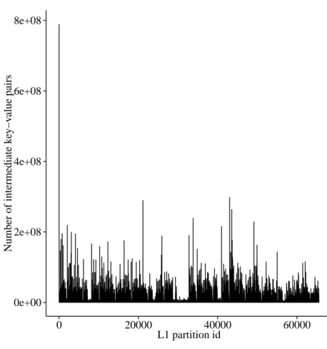
Load balancing. Unlike conventional hash functions, the minimum substring partitioning scheme is locality sensitive, and its main purpose is to maximize the probability of a collision for similar strings. Consequently, the distribution of k-mers across different L1 and L2 parti-tions is severely skewed. Moreover, we have observed that on a number of datasets, almost half of the partitions remain empty. The distribution of intermediate key-value pairs among the non-empty L1 partitions in the Yoruban male dataset can be seen in figure 2.3
There are a few partitions which are much larger than the rest. In the reduce phase where each node handles a subset of the partitions, if the distribution is not uniform, one of the peer nodes of the cluster might get more than its share of data consequently dominating the total execution time, or worse, running out of memory. To tackle this problem, after all reads are processed, the total number of intermediate key-value pairs for each partition is collected from all the nodes, and the partitions are stored in a max-heap based on their sizes. They are then distributed across the nodes using the Longest Processing Time (LPT) scheme.
0e+00 2e+08 4e+08 6e+08 8e+08 0 20000 40000 60000 L1 partition id Number of intermediate k ey−v alue pairs
Figure 2.3. Imbalance of distribution in intermediate data among partitions
Reduce phase. In this phase, each reducer thread picks up one of the L1 partitions assigned to it and starts reducing the values corresponding to each unique key in the list. This reduce phase has two objectives: Firstly, the samek-mer generated from different sequences can have different nucleotides at its ends. These nucleotides which form the incoming and outgoing edges of the vertex represented by thek-mer need to be merged in the final de Bruijn graph. Since the maximum in-degree and out-degree of a vertex is 4, the edges can be encoded in a single byte. Secondly, the number of times ak-mer (regardless of the outgoing edges) occurs in the entire dataset needs to be tracked. This frequency information is used in subsequent stages to recognize erroneous structures in the graph caused by sequencing errors. After this phase, all subgraphs within each partition are locally compressed.
2.3.2. Graph compression phase
Following reduction and local compression, the vertices are distributed among the nodes for further extension. The vertices that have exactly one incoming edge and at most one out-going edge are loaded in a distributed hash map. All other vertices are appended to a dis-tributed list and act as seeds for the extension. After the graph is loaded, the workers traverse the linear chains, starting from the vertices in the list. Each worker looks up the hash map in order to get the next vertex in the chain it is working on.
We guarantee that a single path cannot be traversed by more than one thread making our algorithm lock-free and enhancing scalability. Clearly, there can be an imbalance in load dis-tribution between different threads depending on the lengths of the paths. However, we have observed that with real datasets, the imbalance is not severe enough to warrant the overhead of synchronization.
2.4. Implementation
Our assembler is built on top of ZeroMQ (http://zeromq.org/), which is an embeddable framework for concurrency and communication. It provides a threading library based on He-witt’sActor Model[24] of concurrent computation. The semantics of this model states that an actor is an independent “universal primitive” for concurrency that can only modify its own state and exchange atomic messages with other actors. These concepts differ from the idea of a global state shared by multiple threads, hence actors don’t require locks, semaphores or critical sections.
ZeroMQ also provides an intelligent transport layer for low-latency communication and is best suited for small packets. Moreover, it provides uniform message passing semantics between actors (threads), processes, and boxes (cluster nodes). Accordingly, a pair of ZeroMQ sockets can talk to each other overinproc,ipc, ortcpprotocols.
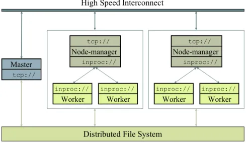
Figure 2.4 shows the high level system overview of Lazer. It consists of a master process, which is responsible for the distribution of tasks, synchronization between nodes and
load-Master tcp:// inproc:// Worker tcp:// Node-manager inproc:// inproc:// Worker inproc:// Worker tcp:// Node-manager inproc:// inproc:// Worker
Distributed File System High Speed Interconnect
Figure 2.4. System overview of Lazer
balancing. Moreover, each node runs a slave process consisting of a Node-manager actor which spawns and manages worker actors. Since a manager and its workers reside in the same address space, they can connect to each other viainprocprotocol. The node-managers connect to the master via tcp. All processes have access to a distributed file system and can send/receive messages to/from each other via a high speed network.
This architecture forms the basis on which all the phases are implemented. The subsec-tions that follow, describe the implementasubsec-tions and actor interacsubsec-tions during each phase in more details.
2.4.1. Map phase
Figure 2.5 shows the different actors at play and their communication patterns during the map phase. The node-manager spawns three types of workers: mappers, partitioners and sinks. All these actors have the same parent process and can communicate viainproc. Mappers ask node-managers for input batches and the request is relayed to the master. On receiving a batch, mapper threads parse the reads into (k+2)-mers (i.e. the k-mer and the nucleotides at its ends). Subsequently, each (k+2)-mer is mapped to one of the available par-titions and sent to the partitioner actor responsible for it. The process is described in Algo-rithm 1.
Master
tcp://rep inproc://req Mapper inproc://push tcp://reqNode-manager
inproc://rep inproc://pull Partitioner inproc://push inproc://req Mapper inproc://push inproc://pull Partitioner inproc://push tcp://dealer inproc://pull SinkLocal Storage
inproc://req Mapper inproc://push tcp://reqNode-manager
inproc://rep inproc://pull Partitioner inproc://push inproc://req Mapper inproc://push inproc://pull Partitioner inproc://push tcp://dealer inproc://pull SinkLocal Storage
Figure 2.5. Actor interactions during map-phase Algorithm 1Mapper actor1: functionMAPPER
2: whilemor e_bat chesdo
3: ZMQ_SEND(manag er,GE T_B AT C H) 4: r ead_bat ch←ZMQ_RECV(manag er) 5: forreadrinr ead_bat chdo
6: t upl e_ar r a y〈kmer,i n,out〉T ←PARSE_READ(r) 7: fortuplek2 inT do
8: 〈PL1,PL2〉 ←MIN_SUBSTR_HASH(k2.kmer)
9: i d←PL1mod|par t i t i oner s|
10: ZMQ_SEND(par t i t i oner s[i d],k2,PL1,PL2)
11: end for 12: end for 13: end while 14: end function
Partitions are maintained as in-memory lists and each partitioner is assigned a subset of those lists. The amount of intermediate data generated at each node is often much more than the memory available. Hence, a subset of the data must be spilled onto disks. Here, we answer the following questions pertaining to data spillage: 1) How do we decide what to spill? and 2) How is the spilled data stored on disk? Assuming there areppartitions, each node begins with
p empty lists. Partitioners receive intermediate key-value pairs from mappers and append them to appropriate lists, according to their minimum substrings. Data is appended to lists in fixed-size chunks, and the total number of chunks across all partitions in a node is tracked. Whenever a new chunk is created, the total chunk count is compared with a threshold, and if it is larger than the threshold, the chunk is spilled to disk. By configuring the threshold, one can limit the memory-per-node that can be used to store the intermediate data. If there is enough memory, intermediate data isn’t spilled onto disk at all, thus removing the I/O bottle-neck during reduction.
Since the data must be spilled in a way that allows entire partitions to be read from the disk at once, storing key-value pairs in flat files is not efficient. Instead, we use a disk-based NoSQL database to index the spilled data. If each partition maintains a current chunk count, the unique keys for the spilled blocks can be generated from the partition id and the chunk id. During reduction, all theniblocks spilled in a partitionPican be retrieved by making GET
calls to the database using keys ranging fromi.0 toi.(ni−1).
We use RocksDB (http://rocksdb.org/) as the underlying NoSQL database. It is an embed-dable persistent key-value store based on log-structured merge trees and can provide a partial ordering of keys based on fixed-length prefixes. Since we dont care how the data is ordered on disk as long as they are grouped by partitions, we can assign the firstl og(p) bits of keys as the prefix. During reduction of a partitionPi, we can iterate over the key-space with prefixi.
Under this scheme, insertion and retrieval perform better than those in databases with total ordering of keys. Furthermore, RocksDB provides a number of useful features such as multi-threaded compactions, thread-safe reads, bloom-filters for caching, and several other
param-eters that can be configured based on the underlying storage system. All of our experiments were run on spinning disks, but we believe the reduce phase will get a significant performance boost if the database is hosted on SSDs. Although RocksDB supports multi-threaded reads, all writes to the database must be serialized. Hence write access to the database is limited to a single actor (sink) that handles all PUT requests from the partitioners, as shown in Figure 2.5 and described in Algorithm 2.
Algorithm 2Partitioner actor 1: functionPARTITIONER 2: c ache←l i st s[|L1|][|L2|] 3: whilemore_kmersdo 4: (k2,PL1,PL2)←ZMQ_RECV(mapper s) 5: LIST_APPEND(c ache[PL1][PL2],k2) 6: ifcache_overflowthen 7: ZMQ_SEND(si nk,c ache[PL1][PL2]) 8: end if 9: end while 10: end function 2.4.2. Reduce phase
Note that in the map phase, there is no communication between nodes. In other words, if there areppartitions, each of the nodes will initially containpbuckets to hold the interme-diate data. This is done in order to achieve a balanced distribution of partitions in the reduce phase. Before the the intermediate data is merged, they must be shuffled around so that for a partitionPi all intermediate data generated withinPi in all the nodes must be moved to the
the node responsible for reducingPi. Figure 2.6 shows how the reducers fetch intermediate
data from the NoSQL database servers located at the different nodes.
Shuffle phase. If the intermediate data is fully contained in memory, the performance of the shuffle phase becomes almost entirely dependent on the network throughput. We have ex-perimentally observed that with the high-speed networks available in most HPC clusters, the memory to memory data transfer does not create any bottlenecks in the process (i.e., the pro-cessor utilization remains fairly high). However, this changes when the intermediate data is
Master tcp://rep inproc://req Reducer tcp://dealer tcp://req Node-manager inproc://rep tcp://router Sink inproc://req Reducer tcp://dealer inproc://req Reducer tcp://dealer tcp://req Node-manager inproc://rep tcp://router Sink inproc://req Reducer tcp://dealer
Local Storage
Local Storage
Figure 2.6. Actor interactions during reduce-phasespilled onto disk. In such scenarios, shuffle performance is dictated by the disk read through-put, which is typically much less than the network throughput. Moreover, if there is a single disk per node, as is the case in most HPC clusters, multiple threads reading from the disk increases contention and adversely affects the performance.
The impact due to disk I/O bottleneck is offset to some extent by using a block pre-fetching scheme on the database server side and a scatter-gather approach on the client side. Both of these features are enabled by ZeroMQ’s high-speed asynchronous messaging engine. On the client side, each reducer starts with a set containing all the nodes and scatters requests for a chunk of intermediate data. This scheme serves two purposes:
1. Since each reducer sends requests to the servers running on all nodes, the database servers share the load uniformly. Moreover, the fact that each reducer only asks for a small chunk prevents starvation of other reducers, albeit at the cost of a higher number of messages in the network.
2. Since messages are transmitted and received asynchronously by ZeroMQ I/O threads, reducers can immediately start working on the chunks as soon as they arrive. Therefore, the latency is reduced to the time between the transmission of the last request to the arrival for the first response.
On the database side, when a server receives a request for a chunk of partitionPi from a
re-ducer, it checks if any blocks inPi reside in memory. Otherwise it fetches one from disk and
responds with it. As the response is being sent, the server checks if the next block is in mem-ory. If it is not, it pre-fetches one from disk. The pseudo-code for the reducer actor is shown in Algorithm 3
An interesting observation worth mentioning at this point is that on some datasets, a sin-gle partition can be so much larger than the others that the reducer handling it might keep on running long after the others are finished. This occurs more often when the program is run on a huge number of cores, where each reducer deals with a very small number number of partitions, most of which have a very small amount of intermediate data, and a select few are massive.
This effect can be seen in figure 2.3, where partition id 0 clearly stands out from the rest. This is an inherent disadvantage of using the minimum substring partitioning scheme, some-thing that comes as a compromise for the reduced memory footprint. Although the effect of these mega-partitions can be somewhat offset when run in a small cluster, they completely destroy the scalability as the number of nodes is increased.
Its apparent that the size of the substring chosen for MSP will have a significant impact of the skewness of the distribution. Thus with some trial-and-error, the substring size can be chosen in a way such that the problem can be alleviated. However, these optimum sizes may widely vary across different datasets. Therefore, the substring size must be fixed by the end user for each new experiment, which is a very undesirable side effect.
To relieve the user of this burden, we only process the smaller partitions with a single thread. All other partitions which are larger than a preset threshold are reduced and locally
Algorithm 3Reducer actor 1: functionREDUCER(PL1) 2: l i st←NU LL 3: forPL2← |L2|t o1do 4: hashmap←MERGE(PL1,PL2) 5: l i st←EXTEND(l i st,hashmap) 6: end for 7: end function 8: procedureMERGE(PL1,PL2) 9: whilenodeset_not_emptydo 10: ZMQ_PUBLISH(nod eset,PL1,PL2)
11: fori=1 to|nod eset|do
12: (n,chunk)←ZMQ_RECV(nod eset) 13: ifchunk_is_emptythen
14: REMOVEFROM(nod eset,n)
15: else
16: add/merge chunk to hashmap 17: end if
18: end for 19: end while 20: end procedure
21: procedureEXTEND(l i st,hashmap) 22: for allvertexv in listdo
23: ifOUT(v)=1 andv.next∈hashmapthen 24: APPEND(v,hashmap[v.next])
25: ERASE(hashmap,v.next) 26: end if
27: end for
28: Move all vertices from hashmap to list 29: end procedure
compressed by all available threads within one of the nodes. After running experiments on a number of datasets we have observed 5×10⁸to be a good threshold value (it can be modified by the user if required). The multithreaded algorithm is very similar to the one described in Algorithm 3, barring a few modifications for synchronization, and is therefore omitted from this text.
2.4.3. Graph compression phase
During this phase, all partitions of the graph must be loaded into memory for further compression and be globally visible to all nodes in the cluster. Moreover, traversal of the graph demands anO(1) lookup of vertices, which implies that they must be stored in a distributed in-memory hash-map. Since, at this stage there are no guarantees that adjacent vertices will reside in the same address space, the traversal may require network communication for every other vertex in the chain which imposes strict latency constraints on the hash-map
We observed that the off-the-shelf distributed hash-tables fail to satisfy the low-latency constraints required for graph traversal, and the low memory footprint we are trying to achieve. Moreover, these general-purpose tools come with features such as load-distribution and fault tolerance, which add extra complexity not necessary for our workload.
To get around these issues, we mimic a distributed hash-map, by using an array of inde-pendent instances of hash-maps running on each node, and a pre-defined hash-function fh
known to all clients. The servers are oblivious to one another, and the clients maintain con-nections to all servers in the cluster. For any key-value pair〈K,V〉, the server id at which the pair will reside is determined byfh(K) modn, wherenis the number of server instances. This
scheme provides a one-hop access to the hash-map since any client would be able toGETa value residing at any node, as long as the key is known to it.
We have chosen Sparsehash (code.google.com/p/sparsehash) as the underlying data structure for the distributed hash-map, since it has the lowest memory footprint. Moreover, using ZeroMQ’s low-latency message transmission and one-hop accesses to each server in-stance, we achieve a high-performance map, even with random accesses on billions of keys.
To increase the throughput even further, we employ an asynchronous pipeline of GET requests, where workers simultaneously work on a batch ofb paths (simultaneously extend
b seeds). At each step, a worker requestsb values from the hash-map corresponding to the outgoing edges of paths in the current batch. Once again, since message transmissions are asynchronous, a request returns immediately with a placeholder for a future result. The ra-tionale here is that if the batch size is large enough, by the time the last request is sent, the response for the first one would have arrived, thus hiding the network latency. When a path reaches its end, it is removed from the batch and replaced with a new seed.
2.5. Evaluation
2.5.1. Overview of datasets
To analyze the performance characteristics of Lazer, we use two different datasets: 1) a synthetic wheat (Triticum aestivum) genome dataset of size 1.1TB from Joint Genome Insti-tute1and 2) a Yoruban male genome dataset of size 452GB from National Center for Biotech-nology Information2. During the process of assembly, the first dataset (i.e., the wheat genome) produces more than 4 TB of temporary data, whereas the second one (i.e., the human genome) produces almost 750GB.
2.5.2. Overview of experimental testbed
To evaluate the performance of Lazer in a distributed environment, we use QueenBeeII3 supercomputing cluster located at LSU. Each compute node of QueenBeeII has two 10-core 2.8 GHz E5-2680v2 Xeon processors, 64GB DRAM and 500GB hard disk drive. Although Queen-BeeII has a total of 480 nodes with this configuration, only 128 of them are available for run-ning a single job. All the nodes are connected by a 56Gb/sec InfiniBand (FDR) interconnect with 2:1 blocking ratio.
1https://gold.jgi.doe.gov/projects?id=Gp0039864 2http://www.ncbi.nlm.nih.gov/sra/?term=SRA000271
2.5.3. Demonstrating the scalability of Lazer
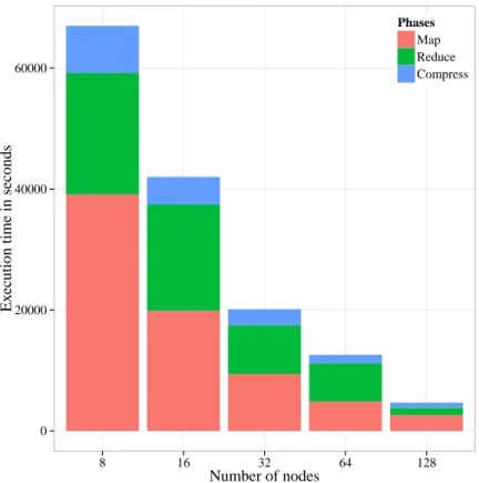
Assembly of wheat genome (1.1TB). To demonstrate the scalability of Lazer, we first assem-ble the relatively larger wheat genome (1.1TB) with different number of nodes in QueenBeeII cluster. Figure 2.7 shows the execution time of different phases of Lazer while assembling the wheat genome. Neither Ray nor SWAP could assemble the 1.1 TB wheat dataset with 128 nodes due to insufficient memory or wall-clock timeout in the cluster.
0 20000 40000 60000 8 16 32 64 128 Number of nodes Ex
ecution time in seconds
Phases Map Reduce Compress
Figure 2.7. Execution times of Lazer on the synthetic wheat W7984 dataset (1.1 TB) Note that the map phase is the most scalable of all phases which is not surprising since this phase is embarrassingly parallel and there is no network communication involved in it. It can also be observed that the compression phase makes up a small fraction of the total ex-ecution time and is also scalable even though it involves a distributed key-value store which in-turn is dependent on network latency. We speculate that the asynchronous pipelined ac-cesses to the hash-map and the lock-less traversal algorithm have a significant impact on the scalability of compression.
On the other hand, the reduce phase appears to scale worse than the others due to the large amount of spilled intermediate data that must be shuffled during reduction. Since each node has a single disk, it presents a bottleneck while reading data and prevents a high CPU utilization.
It is worth mentioning here that we could not assemble this dataset using any other as-sembler even when using the maximum amount resources (i.e., 128 nodes of QueenBeeII clus-ter) available to us.
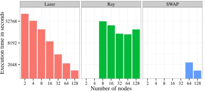
Assembly of human genome (452GB). To compare Lazer’s overall execution time and scal-ability with other assemblers, we used a relatively smaller human genome data set (452GB). Figure 2.8 compares the execution time of Lazer with two other genome assemblers, Ray and Swap while assembling the 452GB human genome. Both axes are in log scale. It can be eas-ily observed that Lazer scales almost linearly with increase in number of nodes whereas Ray cannot complete assembly on 4 nodes and SWAP runs out of memory with 32 nodes.
Lazer Ray SWAP
2048 8192 32768 2 4 8 16 32 64 128 2 4 8 16 32 64 128 2 4 8 16 32 64 128
Number of nodes
Ex
ecution time in seconds
Figure 2.8. Execution times of Lazer, Swap, and Ray on the Yoruban male dataset (452 GB) We were unable to run SWAP on 32 nodes and Ray on 4 nodes due to out-of-memory errors. We observed that Ray’s scalability degrades after 32 nodes, and the execution time increases going from 64 to 128 nodes. Lazer, on the other hand, can assemble the dataset on just 2 nodes, and yet shows a near-linear scalability when running on different configurations.
2.5.4. Demonstrating memory-efficiency of Lazer
The memory efficiency of Lazer is evident from the fact that we could not run the 1.1TB wheat genome using the other assemblers even using the maximum amount of resources available to us i.e., 128 nodes of QueenBeeII providing 8TB (64GB ×128 nodes) of aggre-gated DRAM. On the other hand, Lazer was able to assemble it using only 8 nodes i.e., 512GB (64GB×8 nodes) of memory. Figure 2.8 also demonstrates the memory efficiency of Lazer compared to Ray and Swap 4. It is apparent that Lazer successfully assembles the human genome using only 2-nodes i.e., 128GB (64GB×2 nodes), whereas Ray fails to complete using 4-nodes (i.e., 64GB×4 nodes=256GBof DRAM) or higher. SWAP, although better than Ray in terms of execution time, was found to be the least memory efficient in our evaluation. It re-quires at least 16 times more aggregate memory than Lazer since it runs out on memory with 32 nodes (i.e. 64GB×32 nodes=2T Bof DRAM).
As mentioned earlier, there is a significant imbalance in the size of the partitions can eas-ily overwhelm the hardware resources if they are not carefully distributed among the cluster nodes. In Figure 2.9, we show the distribution of intermediate key-value pairs among peers after the intermediate data is shuffled. It can be observed that the larger partitions are scat-tered across different nodes in a fairly uniform manner so that no single node is assigned more than one. The low memory requirement can be very significant to bioinformatics researchers who may not have access to large scale compute clusters with hundreds of nodes. In such scenarios, Lazer can provide real time solution for assembling huge NGS data set.
2.6. Conclusion
In this chapter, we introduced Lazer, a distributed assembler built using ZeroMQ’s ac-tor and low-latency communication framework that utilizes a smart partitioning scheme for de Bruijn graphs to achieve both scalability and memory efficiency. Experimental results on terabyte-scale datasets show that our framework significantly reduces the memory footprint
4In order to have a fair comparison, we only evaluate the contig generation phases of SWAP and Ray with
0e+00 1e+09 2e+09 3e+09 Nodes(32) T
otal number of intermediate k
ey−v
alue pairs
(a) Distribution on 32 nodes
0.0e+00 5.0e+08 1.0e+09 1.5e+09 2.0e+09 2.5e+09 Nodes(64) T
otal number of intermediate k
ey−v alue pairs (b) Distribution on 64 nodes 0.0e+00 5.0e+08 1.0e+09 1.5e+09 Nodes(128) T
otal number of intermediate k
ey−v
alue pairs
(c) Distribution on 32 nodes
Figure 2.9. Distribution of intermediate key-value pairs with various cluster configurations while ensuring fast assembly. As future work, we plan to add support for reading input data from Hadoop distributed filesystem (HDFS) so that Lazer can be more accommodating to commodity clusters. We also plan to include error removal and scaffolding phases to create a complete assembly pipeline.
Chapter 3. GPU-Accelerated String Graph Assembly
3.1. Introduction
Amidst the extraordinary progress of accelerator technologies we are observing a grow-ing interest in general-purpose GPUs (Graphics Processgrow-ing Units) in various scientific do-mains such as bioinformatics, molecular dynamics, computer vision, and most notably in deep learning. We have also noticed a widening gap between the computational capabilities of general-purpose CPUs and GPUs. For example, the recently introduced NVIDIA Tesla V100 theoretically has 15 TFLOP/s of single precision (FP32) performance and delivers 900 GB/sec peak memory bandwidth, which is an order of magnitude higher than the 85 GB/sec found in the latest Intel Xeon Processor (E7-8894 v4). This meteoric rise of GPUs is very timely, es-pecially when viewed in the context of Next-Generation Sequencing (NGS) technology and its rapid advancement. The increasing size and decreasing cost of raw datasets has made it imperative to utilize hardware acceleration in addition to using general-purpose CPUs to ex-pedite the processing of large genome sequences economically.
Ordinarily, a traditional CPU has a few cores optimized for sequential processing while a single GPU has thousands of cores for massively parallel processing. Several specialized tools have already benefited from the extreme computational capabilities of GPUs across a wide range of bioinformatics applications. These include NVIDIA’s NVBIO [50], CUSHAW [42], CUSHAW2-GPU [40], BarraCUDA [31], SOAP3 [39], SARUMAN [7], PUNAS [12], and GPU-based tools with optimized BWT (Burrows - Wheeler Transformation) [14, 20] and Smith - Wa-terman algorithm [60]. However, most of these studies focus on read alignment, whereas the problem of sequence assembly is not well-addressed due to the limited device memory sizes in GPUs.
Although few GPU-based genome assemblers have been proposed, they are designed for small error-free simulated datasets which inherently limits their assembly performance. This chapter was previously published by Sayan Goswami et.al. as "GPU-Accelerated Large-Scale Genome Assembly" in 2018 IEEE International Parallel and Distributed Processing Symposium (IPDPS). Reprinted by per-mission of IEEE.
Specifically, the largest dataset they have assembled is in a few tens of gigabytes, which is much smaller than typical human genome datasets. Given that the high computational ca-pability of GPUs has not been fully utilized by existing genome assembly tools, it is crucial to develop a new GPU-based assembly framework that uses adequate techniques to scale up to the size of real-world human genomes without requiring large amounts of expensive comput-ing resources.
Several studies have reported that the most challenging step in genome assembly is build-ing a graph (either a strbuild-ing graph or de Bruijn graph) from the short reads since it requires a lot of computing power and a large amount of memory [43] [10]. Although GPUs can alleviate the computational aspect of this issue, the large memory requirement renders them incapable of processing even the medium-sized datasets produced by sequencers today. To address the fundamental limitation of GPUs in large-scale genome assembly, we present a new GPU-accelerated genome assembler, called LaSAGNA, that can assemble datasets with billions of sequences using a single GPU by building string graphs from approximate all-pair overlaps. LaSAGNA significantly reduces the memory requirement by employing a semi-streaming ap-proach that minimizes the number of disk accesses based on the available memory. It can also run on multiple GPUs across multiple compute nodes to expedite the assembly pipeline.
This work makes several contributions as follows. 1) We develop a new genome assembly framework that can build an approximate overlap graph from a real-world human genome sequence dataset (several hundred GB in size) using a single GPU equipped with only 6 GB device memory. 2) We present a two-level semi-streaming model (from disk to host memory and from host memory to device memory) that effectively utilizes the memory hierarchy to reduce the disk I/O in large-scale genome assembly. 3) We implement a distributed version of LaSAGNA to facilitate faster operation on a cluster of compute nodes. Given that the assembly workload is heavily I/O-intensive, LaSAGNA can benefit from the larger aggregated I/O band-width available in distributed computing. 4) We evaluate LaSAGNA using several real-world genome sequence datasets to exhibit its efficiency in various computing environments. Our
experimental results show that LaSAGNA can assemble a 400 GB human genome dataset in 17 hours using a single GPU (NVIDIA K40).
The rest of the chapter is organized as follows. In Section 3.2, we present an exposition of the related literature followed by our proposed approach and its distributed implementation in Section 3.3. Lastly, we show our experimental results in Section 3.4 and conclude this study in Section 3.5.
3.2. Related Work
GPU-Euler [46] is the first genome assembler built for GPUs, followed by GAGM [26], which proposes paired de Bruijn graph construction and contig generation using a single GPU. Both assemblers were evaluated using small simulated error-free reads generated from bacterial genomes. Another GPU-based de Bruijn graph construction tool [43] proposes a staged graph construction pipeline and reports its results on a 13 GB human chromosome dataset. GAMS [27] is the first string graph-based assembler that uses GPUs and reports the as-sembly of a human chromosome using a 16-node GPU cluster. Some works, such as FAssem [58], have studied the application of FPGAs in assembly, but are also evaluated on small bacterial datasets.
There are many CPU-based assembly tools, and most of them are based on de Bruijn graphs. Since the advent of first-generation assemblers such as Velvet [62] and SOAPden-ovo [44], several assemblers, such as Minia [15] and MEGAHIT [36], have been proposed to use succinct data structures (e.g., bloom filters) to store large graphs in memory. Many dis-tributed assemblers have also emerged to expedite the assembly of high-throughput sequenc-ing datasets. Notable among them are Ray [8] and SWAP [47] built on MPI, Lazer [22] which uses ZeroMQ, Contrail [54] and Giga [32] based on Hadoop, and HipMer [21] based on the global-address space model. Among the string graph-based assemblers, SGA [55] is the only one that can process large datasets on a single node using compressed data structures. To the best of our knowledge, CloudBrush [13] is the only distributed string graph-based assembler, but has only been evaluated on small datasets and is still under development.
3.3. Methodology for GPU-Accelerated Assembly
The most expensive stage in any string graph-based assembler is to find the overlaps be-tween all pairs of reads. In theory, one can generate all suffixes and prefixes fromR, and create two lists of key-value pairs,SandP, using suffixes and prefixes respectively as keys and their corresponding read-IDs (unique identifiers of reads) as values. Next, for each key-value pair
<k,ri>inS, one can add an edgee=(ri,rj,|k|) inGif<k,rj>exists inP.
Naturally, this is not practical since storing all suffixes (or prefixes) for an input of sizen
will requireO(n2) space, wherenis the total number of bases inR. The space can be reduced if the actual suffix (or prefix) is replaced by a tuple<l,f >wherelis the length of the suffix (or prefix) and f is its fingerprint. Therefore, for each<<li,fi >,rj >inS, we can conclude that
an edge exists betweenrj andrkwith a high probability ifPcontains<<li,fi>,rk>.
However, even with fingerprints, the space requirement (i.e.,O(nlog2q) bits whereq is the largest fingerprint value) is often too large to fit in the main memory. Indeed, this approach has been attempted [5] but evaluated only on small simulated low-coverage datasets. This problem intensifies in case of large high-coverage real datasets where the reads have a lot of overlaps and require larger fingerprints to minimize the number of false positive edges.
The situation deteriorates with GPUs since their available device memories are typically an order of magnitude smaller than the main memory of even a mid-range workstation. To address this problem, we present a semi-streaming approach for building the string graph by conceptually dividing the memory hierarchy into a read-only memory, a write-only memory, and a working memory, as depicted in Fig. 3.1.
Read-only memory
Write-only memory Disk Working
memory
The read-only memory can only be read sequentially, whereas the write-only memory can only be written sequentially. Note that both the read- and write-only memories reside on disks, but are treated as separate to suggest that a file cannot be read and written at the same time. The working memory consists of a slower host memory and a faster device memory. Unlike the read- and write-only memories, we allow random accesses in the host memory. However, most of the computation is done on the faster device memory, and we minimize the processing done on the host memory. This two-level streaming model (from disk to host memory and from host memory to device memory) efficiently utilizes the memory hierarchy to reduce the amount of disk I/O and enables large-scale sequence assembly. Fig. 3.2 shows the overview of our assembly pipeline in LaSAGNA consisting of four main phases: map, sort, reduce, and traverse. We describe each phase in detail below.
3.3.1. Map: generate pairs of fingerprints and read-IDs
In this phase, batches of reads are loaded in the GPU where their reverse complements are obtained. Next, for each read and its complement, the fingerprints of all their prefixes and suffixes are generated using the Rabin Karp’s rolling hash. Since short-reads in a sequence dataset are of similar lengths, the fingerprint generation can be easily parallelized by assigning each read to a thread. However, on GPUs, this scheme fails to perform as expected due to excessive memory throttling, a scenario where threads block because of numerous pending memory accesses. Moreover, this scheme does not utilize shared memory.
These issues can be addressed if a block of threads processes each read in parallel. To do so, we express prefix fingerprint generation as a Hillis-Steele scan problem. Here, each batch of reads is processed by a grid of thread blocks where the number of blocks equals the number of reads in the batch, and the number of threads per block equals the read-length. Fig. 3.3 illustrates the execution of the kernel used to generate fingerprints of all prefixes of a read whose length is 10 with a prime modulo (q) value of 13 and a radix (σ) 4. In practice, the radix is a small prime larger than the alphabet size, and the prime modulo is a large prime number.
G
A
T
A
C
C
A
G
T
A
3
0
2
0
1
1
0
3
2
0
3
12
2
8
1
5
4
3
1
8
3
12
11
5
7
3
7
5
0
4
3
12
11
5
8
7
2
11
11
5
3
12
11
5
8
7
2
11
7
2
1
4
3
12
9
10
1
4
3
12
4
04
14
24
34
44
54
64
74
84
9M
R
E
P
f[n]= (f[n] + f[n-1]*M[1])%13 f[n]= (f[n] + f[n-2]*M[2])%13 f[n]= (f[n] + f[n-4]*M[4])%13 f[n]= (f[n] + f[n-8]*M[8])%13Figure 3.3. The communication and computing patterns while generating prefix fingerprints ofGATACCAGTAwith radix 4 and prime 13.
Before the kernel is launched, the place values (e.g.,σ0,σ1) for all positions of the read are computed, and their remainders after division by the prime numberqare stored in an array M. This step is done once for the entire program and reused for all reads. In the beginning, each thread in the grid encodes the corresponding base in the read (R=GATACCAGTA) to the radixσ (σ= 4) and places it in its corresponding position in array E. Next, each thread iteratively adds its element to the product of previous element (the current offset determines the previous element), and its place value. Theoffset starts at one and is doubled at every step until its length becomes larger than the read itself. At the end of the algorithm, each positioni in the output array P will store the fingerprint of the prefix ending at positioni (i.e., fingerprint of the prefix of lengthi+1). For example, in Fig. 3.3, the fingerprints ofG,G A, andG AT are 3, 12, and 11 respectively.
The suffix fingerprints are computed using the place values (M) and prefix fingerprints (P) calculated during the previous step as shown in Fig. 3.4. As before, the positioni will now store the fingerprint of the suffix starting from positioni. For instance, in Fig. 3.4, the fingerprints ofGATACCAGTAandATACCAGTAare 2 and 5 respectively.
3 12 11 5 8 7 2 11 7 2 P 2 36 36 44 5 80 63 24 33 28 P’ *M[9] *M[8] *M[7] *M[6] *M[5] *M[4] *M[3] *M[2] *M[1] 2 10 10 5 5 2 11 11 7 2 P’ 2 5 5 10 10 0 4 4 8 0 S S[i]= (2+13-P’[i])%13 P’[i]= P’[i]%13
Figure 3.4. The communication and computing patterns while generating suffix fingerprints using prefix fingerprints
This scheme reduces the number of memory transactions and raises the functional unit utilization of GPUs. Moreover, prefixes and suffixes are processed in a single kernel using shared memory, thus improving performance and avoiding scattered writes during suffix fin-gerprint generation.
Partitioning. To find overlaps between suffixes and prefixes, their lengths (j) and source read-IDs (ri) are appended to their fingerprints (fij) to create a set of 3-tuples. Since we need to find matches between suffixes and prefixes of the same length, it is logical to partition these tuples by their length. Therefore, we sort all (fij,ri) pairs by their corresponding lengths j and count the number of occurrences of each unique j to obtain the size of each partition. In other words, the partitioning process converts a list of (j,fij,ri) tuples tolmaxlists of (fij,ri) tuples, wherelmaxis the length of the sequences. Out of these lists, the ones corresponding to
a length smaller than a user-defined minimum overlap-length (lmi n) are discarded. Moreover,
the partition belonging tolmaxis also dropped to avoid self-loops in the graph. The remaining
3.3.2. Sort: sort read-IDs by fingerprints
To enable binary searches of suffixes in a list of prefixes, in this phase we sort read-IDs by their fingerprints belonging to each partition corresponding to lengthli ∈[lmi n,lmax). Since
the number of suffixes/prefixes is much larger than the GPU memory, we use an external-memory sorting scheme comprising two phases. In the first phase, chunks of key-value pairs (of sizeM such thatM elements fit in GPU memory) are read from disk, sorted by keys, and written back to disk. In the next phase, these chunks are iteratively merged into a single sorted one.
Note that the size of the chunks being merged will double every iteration, and hence the merging must also be done using external-memory. Algorithm 4 explains our approach to combine two sorted lists on disk, by processing at least M/2 and at mostM elements at a time. It is adapted from thek-way mergingscheme and operates under the guiding principle that the input cannot be randomly accessed.