Stela: on-demand elasticity in distributed data stream processing systems

(1)

(2)

STELA: ON-DEMAND ELASTICITY IN DISTRIBUTED DATA STREAM PROCESSING SYSTEMS

BY LE XU

THESIS

Submitted in partial fulfillment of the requirements for the degree of Master of Science in Computer Science

in the Graduate College of the

University of Illinois at Urbana-Champaign, 2015

Urbana, Illinois

Advisor:

(3)

ABSTRACT

Big data is characterized by volume and velocity [24], and recently several real-time stream processing systems have emerged to combat this challenge. These systems process streams of data in real time and computational results. However, current popular data stream processing systems lack the ability to scale out and scale in (i.e., increase or decrease the number of machines or VMs allocated to the application) efficiently and unintrusively when requested by the user on demand. In order to scale out/in, a critical problem that needs to be solved is to determine which operator(s) of the stream processing application need to be given more resources or taken resources away from, in order to maximize the application throughput. We do so by presenting a novel metric called "Expected Throughput Percentage" (ETP). ETP takes into account not only congested elements of the stream processing application but also their effect on downstream elements and on the overall application throughput.

Next, we show how our new system, called Stela (STream processing ELAsticity), incorporates ETP in its scheduling strategy. Stela enables scale out and scale in operations on demand, and achieves the twin goals of optimizing post-scaling throughput and minimizing interference to throughput during the scaling out/in. We have integrated the implementation of Stela into Apache Storm [27], a popular data stream processing system.

We conducted experiments on Stela using a set of micro benchmark topologies as well as two topologies from Yahoo! Inc. Our experiment results shows Stela achieves

(4)

45% to 120% higher post scale throughput comparing to default Storm scheduler performing scale out operations, and 40% to 500% of throughput improvement comparing to the default scheduler during scale in stage. This work is a joint project with Master student Boyang Peng [1].

(5)

(6)

ACKNOWLEDGMENTS

I would like to thank my advisor, Indranil Gupta, to provide invaluable support, inspirations, and guidance for my research during my study. I am also very grateful to him for his millions of suggestions and corrections to help me to improve my writing skill. I would like to thank Boyang Jerry Peng for his collaboration in this project [1]. This work will not be possible without them.

I would also like to express my sincere gratitude to all former and current members of Distributed Protocols Research Group (DPRG), for their constant support like a family. Working with them has been one of the most pleasant experiences and my graduate school career would never be successful without their research suggestions, career advice, and snack support.

I would like to thank my parents for their love, also for showing me that there are no shortcuts to success but endless effort.

Many thanks to our collaborators at Yahoo! Inc. for providing us the Storm topologies: Matt Ahrens, Bobby Evans, Derek Dagit, and the whole Storm development team at Yahoo! Inc.

(7)

In the past decade we have witnessed a revolution in data processing systems. Many large-scale distributed data processing systems [2-7] have evolved from single platform, single data source processing to handling massive datasets characterized by their volume, velocity and variability [24]. Systems like Hadoop have evolved and matured to handle huge volume of batch data [25] by adapting distributed processing paradigm like MapReduce [26]. However, these systems can only serve static data, which makes it impossible for users to retrieve computational results in real time. Furthermore, today’s big data that arrives at a very high rate, such as Twitter [55] feeds, server history logs, and high frequency trading data, which raises new challenges for systems to transmit, compute, and store data in real time [48].

The demand has arisen for frameworks that allow for processing of live streaming data and answering queries while being requested. The development of stream processing systems (SPSs) can be traced back to 1960s [49]. In 1974 Gilles Kahn defined a parallel program schema that can be defined by a labeled nodes and edges in a graph, which is still widely used as data model for SPSs development today [50]. In the 1980s dataflow and SPS became active research areas. SPSs were widely used in

(10)

programing language research, signal processing network and hardware design [49]. Before the era of big data in 21st century, the concept of stream processing has already been popular and frequently used in many areas such as trading systems and online auctions [51-52].

One of the earliest works related to stream processing within a distributed framework was the FOCUS project, published in 1992 [53]. FOCUS treated the distributed system as consisting of concurrent asynchronous processing elements [49]. Meanwhile, several research projects regarding system’s task migration [54] and load sharing [55-56] were conducted, laying a foundation for the development of modern distributed stream processing systems such as Aurora [8] and Borealis [20].

Over the last few years, stream processing has once again become a highly popular topic: systems like Storm [27], System S [22], Spark Streaming [23], Heron [28] and many other systems [9-12] have been developed to facilitate online algorithms for streaming data input. For instance, Yahoo! Inc. uses a stream processing engine to perform for its advertisement pipeline processing, so that it can monitor ad campaigns in real-time. Twitter uses a similar engine to compute trending topics [27]. Other examples include spam detection, personalization, online recommendation and data analytics using real time machine learning algorithms [40].

(11)

Unfortunately, current stream processing systems used in industry largely lack an

ability to seamlessly and efficiently scale the number of servers in an on-demand manner,

while on-demand is defined by the ability to scale upon user’s requests. There are many use cases where shifting the size of cluster is desired. The ability to increase or decrease cluster size on demand without interrupting workload is critical. It helps the users to add hardware resources accordingly when required by scaling out, e.g., when incoming data rate rises. It can also help to reduce unnecessary power and resource consumption by scaling in, e.g., when the system is under-utilized. Without this feature, users have to be stop or pause the application for hardware reconfiguration. This may cause long periods of low or zero throughput. For instance, Storm simply supports such a request by un-assigning all processing operators and then reassigns them in a round robin fashion to the new set of machines. This is not seamless as it interrupts the ongoing computation for a long duration, and shuts down throughput to zero. It is not efficient either as it results in sub-optimal throughput after the scaling is completed as our experiments show later. The recent published system Heron [28] has improved Storm’s architecture from multiple aspects. However the work has not addressed the lack of ability to scale on demand.

In order to bridge this gap, we propose a new metric, Effective Throughput percentage (ETP), to measure the impact of each computational operator on entire application throughput. ETP takes into account not only congested elements of the stream processing application but also their effect on downstream elements and on the overall application throughput. Using ETP metric, our approach is able to determine the operator or machine that affect throughput the most.

(12)

We further present a system, Stela (STream processing ELAsticity) to enable on-demand scaling for distributed data stream systems using ETP metric. Stela meets two design goals: First, it optimizes the post-scaling throughput without hardware profiling. Second, Stela introduces minimal interruption to the ongoing computation. For scale-out, Stela uses ETP metric to select which operators (inside the application) are given more resources based on their impact to the throughput, and secondly it performs the scale-out operation in a way that is minimally obtrusive to the ongoing stream processing. Similarly, for scale in, Stela uses ETP metric to select which machine to remove in a way that minimizes the overall detriment to the application’s performance.

1.3 Contributions Of This Thesis

In this thesis we first introduce the design of our ETP metric. Then we introduce development of our system Stela, that performs scale out and scale in using ETP metric. We integrated Stela into Apache Storm. And finally we present experimental results using both micro-benchmark Storm applications as well as Storm applications from Yahoo!. Our experiments show that compared to Apache Storm’s default scheduler, Stela’s scale out operation reduces interruption time to a fraction as low as 12.5% and achieves throughput that is 45-120% higher than Storm’s. Stela’s scale in operation chooses the right set of servers to remove and performs 40-500% better than Storm’s default strategy.

(13)

• The development of a novel metric, Expected Throughput Percentage (ETP), that accurately captures the “importance” of an operator towards entire application.

• Integrating ETP metric into Storm to achieve maximized throughput with

lower cost.

• Evaluating Stela with default Storm and alternative strategies using both micro-benchmark topology and application used by Yahoo! in production.

(14)

2. RELATED WORK

Aurora [8] was one of the earliest distributed data stream processing systems. Both Aurora and its successor, Borealis [20] used a technique called load shedding to reduce congestion in their workloads. In order to guide load shedding process, they constantly collected QoS information as a metric to detect throughput bottleneck. They also collected hardware statistics to help identify congestion caused by resource shortage. Different from Stela, these systems focused on load balancing of individual machines. Borealis used correlation-based operator distribution to maximize the correlation between all pairs of operators within the workflow [29]. Borealis also used ROD (resilient operator distribution) [30] [9] to determine the best operator distribution plan that does not easily become overloaded under shifting data flow. Comparing to Aurora, Borealis allowed queries to be revised and modified dynamically. However, to our best knowledge, these two systems, as well as some of the most popular distributed stream processing systems such as Storm [27], Samza [36], Heron [28], Spark Streaming [23] [37], MillWheel [47] do not currently optimize for scale out and scale in explicitly.

Stromy [18] was a multi-tenant distributed stream processing engine that supported elastically scaling. Different from traditional stream processing system like Aurora[8] and Borealis [20], Stormy adapted Distributed Hash Table (DHT) [32], a technique from several distributed storage systems [33-35] into its design. Stormy used DHT to map queries (operators) and incoming events to the same physical location using

(15)

a global unique SID. The technique Stormy used for scale in and scale out is called Cloud Bursting. A cloud bursting leader would decide whether or not to introduce/remove nodes to the system based on hardware statistics of each member node. When a new machine was added to the system, it took a random position on the logical ring and took over portions of the data range of its neighbors, which might not be the best option to optimize application throughput.

StreamCloud [15] [31] was a data streaming system designed to be elastic and scalable. StreamCloud was built on top Borealis Stream Processing Engine [9] aimed to support elasticity in the existing Borealis system. Similar to Stela, StreamCloud also adapted parallelization approach. However, StreamClouds focused on the technique to divide user’s query and maintaining stateful operators. The system monitored CPU usage for each sub-cluster and increased/decreased resources for each sub-query. Comparing to Stela, StreamCloud was more concerned with query-based optimization and resource usage for each sub-cluster/machine rather than optimized throughput for the entire workflow.

System S [22] [14] [19], SPC [10] [17] (part of System S), and SPADE [13] (declarative stream processing engine of System S) were developed by IBM to support user-defined massive volumes of continuous data streams [43]. These systems detected workload changes by constantly monitor the peak rate of each operator. Then they expanded or contracted operator’s parallelism to adapt these changes. Similar to StreamCloud, System S also concentrated on elastically scaling in order to optimize per-operator performance, while Stela applies novel ETP metric to the entire workflow.

(16)

System S, Stormy and StreamCloud were not the only stream processing systems that have adapted parallelization approach. Newly developed systems such as [44] and DRS [45] used parallelization for elasticity scaling. These systems changed operator’s parallelization level by QoS metrics [44] or existing models [45-46]. However, systems like [44] and DRS used strategies that optimized for shortest latency, while Stela targets at maximum throughput. More importantly, Stela targets on on-demand elasticity, which implies that the amount of resources to be added (or removed) is determined and restricted by user. This scenario is common to many use cases when users are restricted by their budget or has a plan to use specific amount of resources, which enforces Stela to choose the best operator/machine during scaling.

In a recent paper [18] on adaptive scheduling in Storm, the author’s presented the use of link-based techniques to schedule Storm topologies. By using both topology-based and traffic-based scheduling, the system aimed at minimizing the traffic among executors within same workers. Based on our research, this is only paper at this time that demonstrated effective scheduling techniques (e.g. using link-based scheduling techniques), which surpassed the performances of Storm’s default scheduler. Thus, we choose to compare Stela against strategies using link-based approaches on top of comparing against Storm’s default strategies.

(17)

3. DATA MODEL

In this chapter, we introduce the system model for data stream processing systems in our work. This includes a brief introduction of the workflow input and the important concepts that apply to different types of stream processing systems in general.

3.1 Data Stream Processing Model

Data stream processing model can logically be depicted as a directed acyclic graph (DAG) composed by a set of vertices connected by edges. An example of data stream is illustrated in the Figure 1. In this work, we define such logic graph as a workflow.

(18)

We further define some important concepts in data stream model as follows: Tuple: A tuple is the basic unit being processed within workflow. A tuple can be defined in predefined data type (e.g. Integer, String, etc.) or customized data type (e.g. user-defined class).

Operators: In the workflow DAG, the vertices connected by edges are called operators. An operator is a logical representation of the piece of code provided by the user in the workflow. Each operator can be interpreted as a “step” to execute tuples. Operators can have one or more input which allows it to receive tuples from upstream objects. Similarly, they can deliver their tuples to one or more downstream operators. An operator that has no parent is called a source. An operator that has no children is called a sink. In this work, we assume all operators are stateless: i.e. operators store no information from the previously processed tuples.

Instance: An instance (of an operator) is an instantiation of the operator’s processing logic and is the physical entity that executes the operator’s logic. In general, executors are implemented by processes or threads in order to parallelize the workload for an operator. For each operator, there can be one or more instances executing the program logic simultaneously.

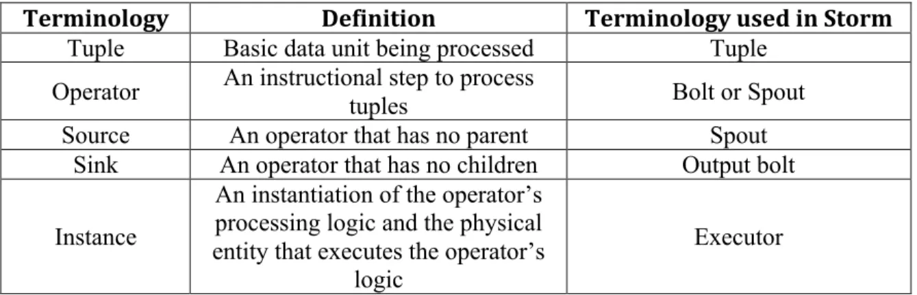
Table 1 lists definitions of theses terminologies. We also include the name of each terminology used in Apache Storm [27], which will be discussed later in Chapter 6.

Terminology Definition Terminology used in Storm

Topology Logical workflow graph Topology Table 1 List of terminologies and their definitions.

(19)

Terminology Definition Terminology used in Storm

Tuple Basic data unit being processed Tuple

Operator An instructional step to process

tuples Bolt or Spout

Source An operator that has no parent Spout

Sink An operator that has no children Output bolt

Instance

An instantiation of the operator’s processing logic and the physical entity that executes the operator’s

logic

Executor

Table 1 List of terminologies and their definitions (continued).

(20)

4. EXPECTED THROUGHPUT PERCENTAGE

In this chapter, we introduce a new metric, called Expected Throughput

Percentage (ETP). ETP estimates the effect of each congested operator of the stream processing application on the overall application throughput. We use ETP to determine which operator to give resources to (while scaling out) or take resources away from (while scaling in). We will first define this metric and describe the algorithm to computed ETP in Section 4.1 and 4.2. Later we will further illustrate computing ETP by an example in Section 4.3.

4.1 Congested Operators

Aiming to achieve high post-scale throughput and low throughput reduction during scaling, our approach consists of two parts: first, we profile the rate of tuples being processed by each operator. Then we create a preferential ordering of the operators in the workflow that determines their priority in scaling out/in.

We consider an operator to be congested if the sum of the speeds of its input streams (input speed 𝑅_!"#$%) is higher than the execution speed 𝑅_!"!#$%! (execution speed). To collect input speed and execution speed for each operator, we periodically records the number of tuples being processed, 𝑇_!"!#$%! and the number of tuples being

(21)

submitted, 𝑇_!"#$, within a sliding time window. For an operator that has 𝑛 parents, we calculate input speed and execution speed as follows:

𝑅_!"#$% = 𝑇!_!_!"#$ ! ! 𝑊 ! !!! 𝑅_!"!#$%! =𝑇!"!#$%! 𝑊

𝑇_!_{_}_!_{_}_!"#$ is the emit rate of parent 𝑖 at time slot j and the number of time slots in a

time window, i.e. window size, is 𝑊.

Our approach detects congested components by Algorithm 1. All congested operators are stored in a data structure called CongestedMap:

Algorithm 1Detecting heavily congested operators in the topology

1: procedure CONGESTIONDETECTION

2: for each Operator o ∈ Topology do

3: 𝑅!"#$% ← 𝑃𝑟𝑜𝑐𝑒𝑠𝑠𝑖𝑛𝑔𝑅𝑎𝑡𝑒𝑀𝑎𝑝(𝑜.𝑝𝑎𝑟𝑒𝑛𝑡); //summing of emit rate of all parents

4: 𝑅_!"!#$%! ← ProcessingRateMap(o);

5: if 𝑅_!_!"#$/𝑅_!"!#$%! > CongestionRate 𝛼 then 6: add o to CongestedMap;

7: end if

8: end for

9: return CongestedMap;

10: end procedure

Here an operator is considered to be congested when 𝑅_!"#$%> 𝛼∗𝑅_!"!#$%!. Here 𝛼 is the congestion rate, a user-defined variable defines the sensitivity of

(22)

congestion detection. We recommend users set 𝛼 to be higher than 1 to compensate for inaccuracies in measurement. For our experiments, we set 𝛼 to be 1.2. A higher congestion rate may lead to less operators being detected by filtering out operators whose input speed is only slightly higher than execution speed.

4.2 Expected Throughput Percentage

Expected Throughput Percentage (ETP) is a new metric we use to evaluate the impact that each operator has towards the application throughput. For any operator x, we define ETP of x as the percentage of the final throughput being affected by the change of 𝑅!, the execution speed of operator x. Formally, we define ETP of operator o in a workflow as:

𝐸𝑇𝑃! =

𝑇ℎ𝑟𝑜𝑢𝑔ℎ𝑝𝑢𝑡!""#$%&'#(#)$!!"#$%&'()

𝑇ℎ𝑟𝑜𝑢𝑔ℎ𝑝𝑢𝑡_!"#$%&"!

We denote the throughput of entire workflow as 𝑇ℎ𝑟𝑜𝑢𝑔ℎ𝑝𝑢𝑡!"#$%&"! and where 𝑇ℎ𝑟𝑜𝑢𝑔ℎ𝑝𝑢𝑡_!"#$%&"! is the sum of the execution speeds of all sinks in the workflow where x resides. To compute 𝑇ℎ𝑟𝑜𝑢𝑔ℎ𝑝𝑢𝑡!""#$%&'#(#)$!!"#$%&'(), which is

(23)

Algorithm 2Find ETP of operator x of the application 1: procedure FINDETP(ProcessingRateMap)

2: if x.child = null then

3: return ProcessingRateMap.get(x) //x is a sink

4: end if

5: SubtreeSum ← 0;

6: for each descendant child ∈x do

7: if child.congested = true then

8: continue; // if the child is congested, give up the subtree rooted at that

child 9: else 10: SubtreeSum+ = FINDETP(child); 11: end if 12: end for 13: return SubtreeSum 14:endprocedure

This algorithm traverses all descendants of operator x and computes the sum of the execution speed of the sinks, only if the sink can be reached by one or more uncongested path(s). It explores the descendent substructure of operator x in depth-first fashion. Here we define substructure of operator x as all downstream operators that receive data stream previously processed by operator x. For example, if the downstream operators descend from operator x forms a tree. Then the substructure of operator x is the subtree rooted at x.

If the algorithm encounters a congested operator, it will prune this substructure and consider this substructure to generate no significant on overall application throughput. Otherwise the algorithm will continue visiting the current explored operator’s children. If this process reaches an uncongested sink operator, it will consider the tuples

(24)

produced by this operator contribute to “effective throughput” and therefore include its execution speed in the ETP of operator x.

4.3 ETP Calculation: An Example

We use an example to show how to calculate ETP of an operator in an application workflow, as shown in Figure.2.

Figure. 2 An example of stream processing application with a tree structure: Shaded operators are congested

In this example, the execution speed for each operator is shown in the figure. The congested operators are shaded and we assume the congestion rate 𝛼 equals to 1, i.e. operators 1, 3, 4 and 6. Thus an operator is congested if the sum of its input speeds is

(25)

higher than the execution speed. Before we calculate the effective throughput of any operators, we first calculate the sum of execution speed of all sinks in the workflow, i.e. 4, 7, 8, 9, 10, as the workflow throughput: 𝑇ℎ𝑟𝑜𝑢𝑔ℎ𝑝𝑢𝑡_!"#$%&"! =2000+1000+ 1000+200+300= 4500 𝑡𝑢𝑝𝑙𝑒𝑠/𝑠.

To calculate the ETP of operator 3, we first determine the reachable sink operators for operator 3 are 7, 8, 9 and 10. Of these only operators 8 and 9 are considered to be the “effectively” reachable sink operators, as both of them can be reached through an uncongested path (through uncongested operator 5). Changing execution speed of operator 3 will affect the throughput of operator 7 and 8 immediately. Meanwhile, operators 9 and 10 will not be affected by the changes despite the fact that both operators are reachable sinks for operator 3. This is because operator 6 being congested suggests that its computational resources have become saturated. Thus, simply increasing execution rate of operator 3 will only make operator 6 further congested. Without providing extra computing resources to operator 6, the input speed for operator 9 and 10 will remain unchanged. We ignore the subtree of operator 6 while calculating 3’s ETP as

ETP_{3 = (1000 + 1000)/4500 = 44%.}

Similarly, for operator 1, operator 4, 7, 8, 9, 10 are sink operators that are reachable. However, none of them can be reached via an uncongested path. Thus the ETP of operator 1 is 0. This implies while the throughput (execution speed) of operator 1 changes, none of the output sink will be affected. Likewise, we can calculate the ETP of operator 4 as 44% and the ETP of operator 6 as 11%. This result suggests when the execution speed of operator 4 changes, 44% of output of the application will be affected.

(26)

For operator 6, only 11% application output will be affected while its execution speed changes.

(27)

5. SCALE OUT AND SCALE IN

By calculating the ETPs of operators, our approach learns the impact each operator has towards the application throughput. In this chapter, we further discuss how our system called Stela uses ETP to support scale out and scale in an on demand manner.

5.1 Goals

There are two goals that Stela aims at during its scaling process: 1. Achieve high post-scale throughput and

2. Minimize the interference towards the running workflow.

In order to achieve these two goals, we use ETP metric to determine the best operator to parallelize and migrate to the new machine(s) during scale out operation, or the best machine(s) to remove during the scale in operation. Here we define scale out as the system’s ability to reallocate or re-arrange part of its current jobs to newly added machines. Similarly, we define scale in as the system’s ability to select machine(s) to remove from the current cluster, and reallocate or re-distributed tasks to the remaining machines. All scaling decisions can be made without hardware profiling. The details of these policies are described in the following sections.

(28)

5.2 Scale Out

This section introduces how Stela performs a scale out operation when new machine(s) are added to the system. Upon receiving user’s request for scale out, we first determine the number of instances it can allocate to new machine(s) and prepares its operation by collecting the execution speed and input speed for each operator. Then it calculates the ETP for each congested operator and capture the percentage of total application throughput that the operator has impact on. Finally we iteratively select the “best” operator to assign more resources by increasing its parallelism level. We describe these details below.

5.2.1 Load Balancing

Stela first determines the amount of instances it needs to allocate to the new machine(s) when the scale out request is received. To ensure load balancing, Stela allocates new instances to the new machine(s) so that the average number of instances per machine remains unchanged. Assuming before scale out the number of instances in the application is 𝐼_!!"!!"#$% and the number of machines in the cluster is 𝑀_!"#!!"#$%. Stela determines the number of instances to allocate to each new machine as ∆𝐼 =

𝐼!"#!!"#$%/𝑀!"#!!"#$%, where ∆𝐼 is also the average number of instances per machine

(29)

5.2.2 Iterative Assignment

After determining the number of instances to be allocated to the new machine(s). We allocate instance slots on these machines. A list of instance slots is a data structure we define for each machine that stores the executors to be needs to be migrated to the machine. We search for all congested operators in the workflow and calculate their ETPs. All ETPs and the operators are stored in a data structure called CongestedMap in the form of key-value pairs. (See Chapter 3 for details). While assigning new instance to an instance slot, our approach target at the operator with highest ETP in CongestedMap and parallelize it by adding one more instance to the instance slot on a new machine.

Algorithm 3 depicts the pseudocode.

Algorithm 3Stela: Scale-out 1: procedure SCALE-‐OUT 2: slot ← 0;

3: while slot < Ninstances do

4: CongestedMap ← CONGESTIONDETECTION; 5: if CongestedMap.empty = true then

6: return source; // none of the operators are congested

7: end if

8: for each operator o ∈ CongestedMap do 9: ETPMap← FINDETP(Operator o); 10: end for

11: target ← ETPMap.max;

12: ExecutionRateMap.update(target); //update the target execution rate 13: slot++;

14: end while 15:end procedure

(30)

This iteration repeats ∆𝐼∗∆𝑀 times where ∆𝐼 is the number of instance slots on a new machine and ∆𝑀 is the number of newly added machines. During each iteration we select a target operator to spawn a new instance that will be allocated to the new

machine. The algorithm traverses all congested operators (via CongestedMap) and

computes the ETP value for each operator (using the algorithm described in Chapter 3). Then Stela stores them in ETPMap as key-value pairs sorted by values. Finally it selects the operator with the highest ETP value and sets that operator as a target. If the CongestedMap is empty, meaning there are no operators being congested in the application, Stela will select one of the source operators so that the input rate of the entire workflow will be increased – this will increase rate of incoming tuples for all descendant operators of that source.

Before the next iteration starts, Stela attempts to estimate the execution rate of the previously targeted operator o. It is critical to update the execution rate of the targeted operator since the assigning new resources to a congested operator may affect the input speed for all descendant operators. Thus it is important for it to estimate the execution speed of o and input speed for all descendants of o every iteration. Assuming

target operator has execution speed of 𝐸_! and operated by k instances, we estimate the

execution speed of the target operator proportionally by: 𝐸′_! =𝐸_!∗(𝑘+1)/𝑘. The intuition behind the design choice is clear: by predicting the impact of each congested operator towards the entire application based on the structure of the workflow, we can discover a combination of operators that may generate most benefit to the application by assigning extra resources.

(31)

After the algorithm updates the execution speed of the target operator, it re-runs Algorithm 1 for each operator in the workflow and updates CongestedMap. Then it recalculates the ETP for each operator in the updated CongestedMap. We call these new ETPs as projected ETPs, or PETPs. PETPs are estimated value of ETPs assuming extra resources have been granted to the operator for the current iteration. Each iteration selects the operator with highest ETP to assign an instance slot to accommodate a new instance of this operator. The processes repeats ∆𝐼∗∆𝑀 until all instance slots are assigned, where ∆𝐼 is the number of instance slots on a new machine and ∆𝑀 is the number of newly added machines.

5.3 Scale In

In this section we describe the technique Stela uses for scale in operation using ETP metric. For scale in, we assume the user send the number of machines to be removed along with the scale in request. Different from scale out operation, Stela needs to decide which machine(s) to remove from the cluster and how to re-distribute the jobs resides on these machines. To decide this machine, Stela uses ETP to calculate the ETP of each machine (not just each operator). ETP of one machine is defined by the sum of ETPs of all executors on this machine. ETP of an executor equals to ETP of operator this executor belongs to. For a machine with n instances, Stela computes sum of ETP of all executors for this machine as:

(32)

𝐸𝑇𝑃𝑆𝑢𝑚 𝑚𝑎𝑐ℎ𝑖𝑛𝑒_𝑘 = ! 𝐹𝑖𝑛𝑑𝐸𝑇𝑃(𝐹𝑖𝑛𝑑𝐶𝑜𝑚𝑝(𝑡𝑖))

!_!!

For a specific instance, our approach looks up the operator that spawns this instance. It then invokes FindETP to find the ETP for the operator as well as the instance. Repeating this process for every instance, it stores the ETPSum for each machine then decides which machine(s) to be removed. Algorithm 4 depicts this process.

Algorithm 4Stela: Scale-out 1: procedure SCALE-‐OUT 2: slot ← 0;

3: while slot < Ninstances do

4: CongestedMap ← CONGESTIONDETECTION; 5: if CongestedMap.empty = true then

6: return source; // none of the operators are congested

7: end if

8: for each operator o ∈ CongestedMap do 9: ETPMap← FINDETP(Operator o); 10: end for

11: target ← ETPMap.max;

12: ExecutionRateMap.update(target); //update the target execution rate 13: slot++;

14: end while 15:end procedure

Assuming M_scalein is the number of machines user specifies to remove. The algorithm traverses all machines in the cluster and construct an ETPMachineMAP that stores ETPSum for each machine. ETPMachineMAP is sorted by its value. Stela selects

(33)

target machine(s). We select the machine with lowest ETPSum because, according to our Stela metric, the executors reside on that machine will have the lowest impact on application throughput in total.

Then Stela re-distributes instances from target machines to all other machines in a round-robin fashion in increasing order of their ETPSum. This design is beneficial in two ways: Distributing instances in a round-robin fashion ensures load-balancing. Additionally, while the total number of instances on target machine(s) cannot be evenly distributed to the remaining machine, prioritizing destination machine with lower ETPSum may introduce less intrusion to the workflow. This is the instances reside on machine with lower ETPSum is likely to have less impact on the application.

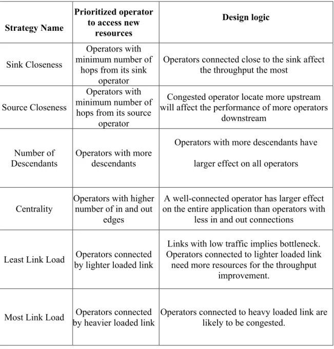
5.4 Alternative Strategies

Besides our scale in and scale out strategy based on ETP metric, we attempt several alternative topology-aware strategies for scaling out. These strategies choose specific operator(s) purely based their alignment in the workflow DAG. Then the chosen operator(s) are reallocated to the new resources in the cluster. We list these strategies in and their design logic in Table 2. Then we will compare the ETP-based approach against them in our experiment section.

(34)

Strategy Name Prioritized operator to access new resources Design logic Sink Closeness Operators with minimum number of

hops from its sink operator

Operators connected close to the sink affect the throughput the most

Source Closeness

Operators with minimum number of

hops from its source operator

Congested operator locate more upstream will affect the performance of more operators

downstream

Number of

Descendants Operators with more descendants

Operators with more descendants have larger effect on all operators

Centrality

Operators with higher number of in and out

edges

A well-connected operator has larger effect on the entire application than operators with

less in and out connections

Least Link Load _{by lighter loaded link}Operators connected

Links with low traffic implies bottleneck. Operators connected to lighter loaded link

need more resources for the throughput improvement.

Most Link Load _{by heavier loaded link}Operators connected Operators connected to heavy loaded link are _{likely to be congested.}

Table 2: Alternative Strategies And Their Design Logic

Among all these strategies, the two link-load based strategies have been used previously [18] to improve Storm’s performance. We also found Least Link Load strategy improves application performance the most during our experiments. Thus we choose Least Link Load to represent all alternative strategies listed above. This is because

(35)

Least Load Strategy aims to minimize the network traffic among physical machines. Thus most of the data transfer between instances can be done locally. In our evaluation section we will compare Least Link Load strategy with our ETP metric approach in terms of throughput performance and degree of workload interruption.

(36)

6. IMPLEMENTATION

Stela is implemented as a scheduler inside Apache Storm [27], an open source distributed data stream processing system [42]. In this chapter we will discuss Stela’s system design and implementation. We will first provide an overview of Storm [41]. Then we will present the architecture and design details of Stela.

6.1 Storm Overview

Apache Storm [27] is an open source distributed real time computation system. Storm is widely used in many areas, such as real time analytics, online machine learning, continuous computation, etc. Storm can be used with many different languages and can be integrated with database in real time.

6.1.1 Storm Workflow And Data Model

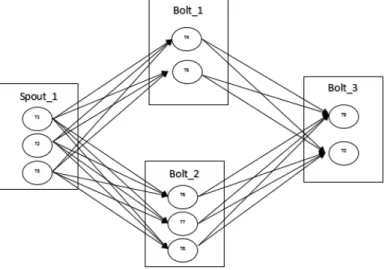
Real time workflow in Storm is called "Stream". In storm, a data stream is an unbounded sequence of tuples. A topology is a user-defined application that can be

(37)

logically interpreted by a DAG of operators. Storm’s operators are all stateless. In a topology, the source operators are called spouts, and all other operators are called bolts. Each bolt receives input streams from its parent spout or bolt, performs processing on the data and emits new stream to be processed downstream. A Storm bolt can perform a variety of tasks such as to filter/aggregate/join incoming tuples, querying database, and any user defined functions. Storm spout or bolt can be run by one or more instances in parallel. In Storm these instances are called executors. A user can specify the parallelism hint of each spout or bolt before application starts. Then Storm will spawn the specified number of executors for that operator upon user’s request. Executors owned by the same operator contain the same processing logic but they are assigned to different machines. Each executor may further be assigned one or multiple tasks. Data stream from upstream operator can be assigned to different tasks based on grouping strategies specified by users. These strategies include shuffle grouping, fields grouping, all groupings, etc.

Figure 3 illustrates the intercommunication among tasks in a Storm topology.

(38)

6.1.2 Storm Architecture

A Storm cluster is composed by two types of node: the master node and work nodes. The master node runs a Nimbus daemon that distributes, tracks and monitors all executors in the system. Each worker node runs a Supervisor daemon that starts one or more worker process(es) and executes a subset of topology. The Nimbus communicates with ZooKeeper [6] to maintain membership information of all Supervisors.

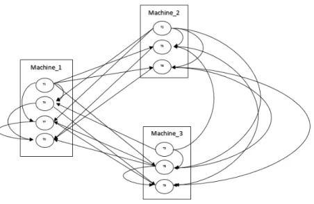
Each Supervisor uses worker slots to accommodate worker processes. In our experiment, each Supervisor may contain up to 4 worker processes. Tasks, along with their executors (as described in 5.1.1), are assigned to these workers. By default, Storm’s scheduler schedules tasks to machines in a round robin fashion. Tasks of one operator are usually placed on different machines.

(39)

Figure 4 depicts a task allocation example of a 3-machine Storm cluster running the topology shown in Figure 3.

Storm scheduler (inside Nimbus) is responsible for placing executors (with their tasks) of all operators on worker processes. Default Storm scheduler supports REBALANCE operation. REBALANCE operation allows users to change application’s parallelism hint and the size of the cluster. This operation creates new scheduling by un-assigning all executors and re-scheduling all executors (with their tasks) in a round robin fashion to the modified cluster.

6.2 Stela Architecture

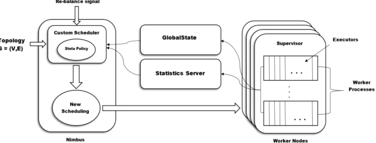
The architecture of Stela is shown in Figure 5.

(40)

Stela is built as a customized scheduler for Storm. It consists of 4 main components:

Statistics Server: Statistics Server is responsible for collecting statistics in Storm cluster. These statistics include: the number of executed tuples and number of emitted tuples of each executor and operator. Statistics Server then passes this information to GlobalStates.

GlobalState: GlobalState is responsible for storing current scheduling information of Storm cluster, which includes where each task or executor is placed in the cluster, the mapping between executor and tasks and the mapping between executor and components. Global States also inquire statistics from Statistics Server periodically and then computes the execution speed and input speed of each bolt and spout. This process is demonstrated in Section 3.1.

Strategy: Strategy implements core Stela policy and alternative strategies (Section 4). It also provides an interface for ElasticityScheduler to easily switch its scale out or scale in policy. Strategy provides a new schedule, i.e. task allocation plan, by policy in use by system information stored in Statistics Server and GloabalState.

ElastisityScheduler: ElasticityScheduler implements IScheudler, a standard API provided by Storm for users to customize Storm scheduler. ElasticityScheduler integrates Statistics Server, Global States and Strategy components and provides new schedule to Storm internal. This scheduler can be invoked by user’s REBALNCE request with scale in or scale out operation specified.

(41)

Stela detects newly added machines upon receiving scale out request. Then it invokes Strategy component to contact Statistics Server and Global Strategy. And final scheduling is returned to ElasticityScheduler by Strategy. Upon receiving a scale in request, Stela invokes Strategy as soon as the request arrives. Strategy component eventually returns a final scheduling as well as a plan to suggest which machine(s) to remove.

(42)

7. EVALUATION

In this section we evaluate the performance of Stela (integrated into Storm) by using a variety of Storm topologies. The experiments are divided into two parts: 1) We compare the performance of Stela (Section 2.1) and Storm’s default scheduler via three micro-benchmark topologies: star topology, linear topology and diamond topology; 2) We present the comparison between Stela, Link Load Strategy (Section 3.3), and Storm’s default scheduler using two topologies from Yahoo!, which we call PageLoad topology and Processing topology.

7.1 Experimental Setup

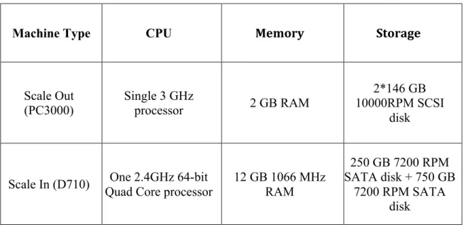
We use Emulab testbed [21] to perform our experiments. We use two types of machines for experiments: for scale out experiments we use PC3000 [38] machines and for scale in experiment we use D710 [39] machines for scale in experiments. All machines in the cluster are connected by 100Mpbs VLAN. We list hardware configurations of these two machine types in Table 3. We further list the Cluster and topology settings and cluster changes during scaling process for each of our experiment in Table 4.

(43)

Machine Type CPU Memory Storage Scale Out (PC3000) Single 3 GHz processor 2 GB RAM 2*146 GB 10000RPM SCSI disk

Scale In (D710) One 2.4GHz 64-bit

Quad Core processor

12 GB 1066 MHz RAM 250 GB 7200 RPM SATA disk + 750 GB 7200 RPM SATA disk

Table 3. Hardware configurations of machines

Table 4. Cluster and topology settings Topology Type Tasks per Component Count Initial Executors per Component Count Worker Processes Count Initial Cluster Size Cluster Size after Scaling Star 4 2 12 4 5 Linear 12 6 24 6 7 Diamond 8 4 24 6 7 Page Load 8 4 28 7 8 Processing 8 4 32 8 9 Page Load Scale in 15 15 32 8 4

(44)

7.2 Micro-benchmark Experiments

We created three basic micro topologies for our scale out experiments. These three micro topologies are commonly used in many stream processing applications. Furthermore, they often serve as sub-component of large-scale data stream DAG. The layouts of these three topologies are depicted in Figure 6.

(a) Star Topology (b) Linear Topology (c) Diamond Topology

Figure 6. Layout of Micro-benchmark Topologies.

For the Star, Linear, and Diamond topologies we observe that Stela’s post scale-out throughput is around 65%, 45%, 120% better than that of Storm’s default scheduler, respectively. This indicates that Stela correctly identifies the congested bolts and paths and prioritizes the right set of bolts to scale out. Figure 7 shows the results of these experiments.

(45)

(a) Star Topology

(b) Linear Topology

(c) Diamond Topology

(46)

Based on Storm’s default scheduling scheme, the number of executors for each operator will not be increased unless requested by users. Our experiment shows migrating executors to new machine(s) does not improve overall throughput. This is caused by two reasons: 1. Providing extra resources to executor that is not resource constrained does not benefit performance, and 2. While the operator is processing at its best performance, its processing can hardly be improved without increasing the number of executors.

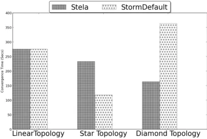
One of the two goals of Stela is to minimize interruption to the running workflow (Chapter 1). We calculate convergence time for all scale out experiments. The results for micro benchmark topologies are presented in Figure 8.

Figure 8. Micro Benchmark Convergence Time: Stela vs. Storm Default

Convergence time measures the interruption imposed by certain strategy to the running workflow. Convergence time is the time interval between when the scale out operation starts and when workload throughput stabilizes. To calculate the ending point

(47)

of the convergence time, we first calculate the average post-scale throughput M and standard deviation 𝜎. We define two types of post-scale data point as effective. Assuming Storm application overall throughput is T at time point P. If 𝑇> 𝑀 and 𝑇−𝑀 < 𝜎, then we define T as a type 1 time data point. If 𝑇< 𝑀 and 𝑀−𝑇< 𝜎, then we define T as a type 2 data point. We further define the time of stabilization as the time when we collect at least two type 1 data points and at least two type 2 data points after scale out. A lower convergence time implies that the strategy is less intrusive during the scaling process.

Base on experiment results, we observe that Stela is far less intrusive than Storm when scaling out in the Linear topology (92% lower) and about as intrusive as Storm in the Diamond topology. Stela has longer convergence time tha Storm in Star topology.

7.3 Yahoo! Benchmark Experiments

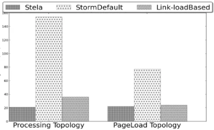
We obtained the layouts of two topologies in use at Yahoo! Inc.: Page Load topology and Processing topology. The layout of these two topologies are shown in Figure 9. We examine the performance and convergence time of three scale out strategies: Storm default, Link load based and Stela. For link load based strategy, we choose Least Link Load strategy since it shows the best post scale throughput among all alternative strategies (Chapter 4.4). Least Link Load strategy reduces the network latency of the workflow by co-locating communicating tasks to the same machine. The result is shown in Figure 10.

(48)

(a) Page Load Topology (b) Processing Topology

Figure 9. Yahoo! Benchmark topology layout

(a) Page Load Topology (b) Processing Topology

Figure 10. Yahoo! Benchmark topology throughput result

From Figure 10, we observe that Stela improves the throughput by 80% after a scale-out for both topologies, while the other two strategies don’t increase the post scale throughput. In fact, Storm default scheduler even decreases the application throughput after scale out. This result is caused by the difference between migration and parallelization, as we have already observed in the previous section (Section 6.2):

(49)

Migrating tasks that are not resource constrained to the new machine(s) will not significantly improve throughput performance. Increasing parallelization or adding additional instances/executors allows operators to consume new resources more effectively. Furthermore, without carefully selecting operator and destination machine, reassigning executors in a round robin fashion can easily cause some machines to be overloaded and creating new bottleneck. Figure 11 shows the convergence time for Yahoo! Topologies.

Figure 11. Yahoo! Topology Convergence Time: Stela vs. Storm Default vs. Least Link Load

In order to minimize interruption to the running workload, Stela makes best effort to not change current scheduling, but rather creates new executors on new machines. Similar to Star topology in our micro benchmark experiment, Stela is much less intrusive than other two strategies when scaling out in both Yahoo! Strategies. Stela’s convergence time is 88% and 75% lower than that of Storm’s default scheduler and about 50% lower than that of Least Link Load strategy.

(50)

7.4 Scale In Experiments

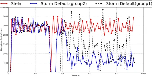
We finally examined the performance of Stela scale in strategy by running Yahoo’s Page Load topology. By default Storm initialize the operator allocation so that executors for the same operator will be distributed to as many as machines as possible. However this may cause the problem less challenging since all machines in the cluster are almost equally loaded. We modified the operator allocation so that each machine can be occupied by tasks from less than 2 operators. We compare performance of Steal and performance of a round robin scheduler (same as Storm’s default scheduler) with two alternative groups of randomly selected machines. During the scale in process we shrink cluster size by 50% (8 machines to 4 machines). Figure 12 shows the throughput changes.

Figure 12. Scale in experiment throughput result: Stela vs. Storm Default

We observe that Stela preserves throughput after half of the machines are removed from the cluster, while the Storm default scheduler experiences 200% and 50%

(51)

throughput decrease depends on operator selection. Thus, Stela’s post scale throughput is 40-500% higher than default scheduler, who randomly chooses machines to remove.

To illustrate scale in process, we further present Storm’s throughput timeline plot in Figure 13. also achieves 87.5% and 75% less down time (time duration when throughput is zero) than group 1 and group 2, respectively. As we discussed earlier (Section 4.4), Stela migrates operators with low ETP to be less intrusive to the application. While the chosen operator has congested descendant, this also allows downstream congested components to digest tuples in their queues and continue producing output. In PageLoad Topology, the two machines with lowest ETPs are chosen to be redistributed by Stela, which generates less intrusion for the application thus significantly better performance than Storm’s default scheduler. Thus, Stela is intelligent at picking the best machines to remove (via ETPSum). In comparison, default scheduler cannot guarantee to pick the “best” operators to migrate every run. In the above scenario, 2 out of the 8 machines were the “best”. The probability that Storm picks both (when it picks 4 at random) is only !_! ÷ !_! = 0.21.

(52)

Figure 13. Scale in experiment throughput result: Stela vs. Storm Default (two groups)

(53)

8. CONCLUSION

We have created a novel metric, which we call as ETP (Effective Throughput Percentage), that accurately captures the importance of operators based on congestion and contribution to overall throughput. We used the ETP metric as a black box to present on demand scale-in and scale-out techniques for stream processing systems like Apache Storm.

For scale out, Stela first selects congested processing operators to re-parallelize based on ETP. Afterwards, Stela assigns extra resources to the selected operators to reduce the effect of the bottleneck. For scale in, we also use an ETP-based approach that decides which machine to remove and where to migrate affected operators.

Our experiments on both micro-benchmarks Topologies and Yahoo Topologies show significantly higher post-scale out throughput than default Storm and Link-based approach, while also achieving faster convergence. Compared to Apache Storm’s default scheduler, Stela’s scale-out operation reduces interruption time to a fraction as low as 12.5% and achieves throughput that is 45-120% higher than Storm’s. Stela’s scale-in operation chooses the right set of servers to remove and performs 40-500% better than Storm’s default strategy.

(54)

Stela provides a solution for distributed data stream processing systems to scale out and scale in on demand. However, in many cases it is necessary for a stream

processing system to scale out and scale in adaptively, i.e. by profiling and adapting to

changing workload, a system can expand/shrink the number of machines so that all machines are best utilized. Thus one important future direction of this work, is to apply ETP metric to distributed stream processing systems to promote systems’ ability to scale out and scale in adaptively. Currently, we propose that the new system should satisfy two SLAs (service-level agreements): 1. Throughput SLA: With minimum throughput requirement, the system minimizes the number of machines involved during scaling process. 2. Cost SLA: With fixed number of machines available, the system maximizes the post-scale throughput for each scaling operation it performs.

(55)

REFERENCES

[1] Peng, B. " Elasticity and resource aware scheduling in distributed data stream processing systems”Master's Thesis, University of Illinois, Urbana-Champaign, 2015.

[2] Apache Hadoop. http://hadoop.apache.org/. [3] Apache Hive. https://hive.apache.org/. [4] Apache Pig. http://pig.apache.org/. [5] Apache Spark. https://spark.apache.org/.

[6] Isard, M., Budiu, M., Yu, Y., Birrell, A., and Fetterly, D. (2007). Dryad: Distributed data-parallel programs from sequential building blocks. In ACM SIGOPS

Operating Systems Re- view, volume 41, pages 59–72. ACM.

[7] Murray, D. G., McSherry, F., Isaacs, R., Isard, M., Barham, P., & Abadi, M. (2013, November). Naiad: a timely dataflow system. In Proceedings of the Twenty-Fourth ACM Symposium on Operating Systems Principles (pp. 439-455). ACM.

[8] Abadi, D., Carney, D., Cetintemel, U., Cherniack, M., Convey, C., Erwin, C., Galvez, E., Hatoun, M., Maskey, A., Rasin, A., et al. (2003). Aurora: A data stream

management system. In Proceedings of the 2003 ACM SIGMOD International Conference on Management of Data, pages 666–666. ACM.

[9] Abadi, D. J., Ahmad, Y., Balazinska, M., Cetintemel, U., Cher- niack, M., Hwang, J.-H., Lindner, W., Maskey, A., Rasin, A., Ryvkina, E., et al. (2005). The design of the Borealis stream processing engine. In CIDR, volume 5, pages 277–289.

[10] Amini, L., Andrade, H., Bhagwan, R., Eskesen, F., King, R., Selo, P., Park, Y., and Venkatramani, C. (2006). SPC: A distributed, scalable platform for data mining. In Proceedings of the 4th International Workshop on Data Mining Standards, Services and Platforms, pages 27–37. ACM.

[11] Loesing, S., Hentschel, M., Kraska, T., and Kossmann, D. (2012). Stormy: An elastic and highly available streaming service in the cloud. In Proceedings of the 2012 Joint EDBT/ICDT Workshops, pages 55–60. ACM.

(56)

[12] Neumeyer, L., Robbins, B., Nair, A., & Kesari, A. (2010, December). S4: Distributed stream computing platform. In Data Mining Workshops (ICDMW), 2010 IEEE International Conference on (pp. 170-177). IEEE.

[13] Gedik, B., Andrade, H., Wu, K.-L., Yu, P. S., and Doo, M. (2008). SPADE: The System S declarative stream processing engine. In Proceedings of the 2008 ACM SIGMOD International Conference on Management of Data, pages 1123–1134. ACM.

[14] Gedik, B., Schneider, S., Hirzel, M., and Wu, K.-L. (2014). Elastic scaling for data stream processing. IEEE Transactions on Parallel and Distributed Systems., 25(6):1447–1463.

[15] Gulisano, V., Jimenez-Peris, R., Patino-Martinez, M., Soriente, C., and Valduriez, P. (2012). StreamCloud: An elastic and scalable data streaming system. IEEE

Transactions on Parallel and Distributed Systems., 23(12):2351–2365. [16] Apache Zookeeper. http://zookeeper.apache.org/.

[17] Jain, N., Amini, L., Andrade, H., King, R., Park, Y., Selo, P., and Venkatramani, C. (2006). Design, implementation, and evaluation of the linear road benchmark on the stream processing core. In Proceedings of the 2006 ACM SIGMOD International Conference on Management of Data, pages 431–442. ACM.

[18] Aniello, L., Baldoni, R., and Querzoni, L. (2013). Adaptive online scheduling in Storm. In Proceedings of the 7th ACM International Conference on Distributed Event-based Systems, pages 207–218. ACM.

[19] Schneider, S., Andrade, H., Gedik, B., Biem, A., and Wu, K.- L. (2009). Elastic scaling of data parallel operators in stream processing. In IEEE International Symposium on Parallel & Distributed Processing, 2009. IPDPS 2009., pages 1–12. IEEE.

[20] Tatbul, N., Ahmad, Y., C ̧ etintemel, U., Hwang, J.-H., Xing, Y., and Zdonik, S. (2008). Load management and high availability in the Borealis distributed stream processing engine. In GeoSensor Networks, pages 66–85. Springer.

[21] Emulab. http://emulab.net/

[22] Wu, K.-L., Hildrum, K. W., Fan, W., Yu, P. S., Aggarwal, C. C., George, D. A., Gedik, B., Bouillet, E., Gu, X., Luo, G., et al. (2007). Challenges and experience in prototyping a multi- modal stream analytic and monitoring application on System S. In Proceedings of the 33rd International Conference on Very Large Databases, pages 1185–1196. VLDB Endowment.

(57)

[23] Zaharia, M., Das, T., Li, H., Shenker, S., and Stoica, I. (2012). Discretized streams: An efficient and fault-tolerant model for stream processing on large clusters. In Proceedings of the 4th USENIX conference on Hot Topics in Cloud Computing, pages 10–10. USENIX Association.

[24] Laney, D. (2001). 3D data management: Controlling data volume, velocity and variety. META Group Research Note, 6, 70.

[25] Bhattacharya, D., Mitra, M. (2013) Analytics on big fast data using real time stream data processing architecture. EMC Proven Professional Knowledge Sharing

[26] Dean, J., & Ghemawat, S. (2008). MapReduce: simplified data processing on large clusters. Communications of the ACM, 51(1), 107-113.

[27] Storm. http://storm.incubator.apache.org/.

[28] Sanjeev Kulkarni, Nikunj Bhagat, Maosong Fu, Vikas Kedigehalli, Christopher Kellogg, Sailesh Mittal, Jignesh M. Patel, Karthik Ramasamy, and Siddarth Taneja. 2015. Twitter Heron: Stream Processing at Scale. In Proceedings of the 2015 ACM SIGMOD International Conference on Management of Data (SIGMOD '15). ACM, New York, NY, USA, 239-250. DOI=10.1145/2723372.2742788

http://doi.acm.org/10.1145/2723372.2742788

[29] Xing, Y., Zdonik, S., & Hwang, J. H. (2005, April). Dynamic load distribution in the borealis stream processor. In Data Engineering, 2005. ICDE 2005. Proceedings. 21st International Conference on (pp. 791-802). IEEE.

[30] Xing, Y., Hwang, J. H., Çetintemel, U., & Zdonik, S. (2006, September). Providing resiliency to load variations in distributed stream processing. In Proceedings of the 32nd international conference on Very large data bases (pp. 775-786). VLDB Endowment.

[31] Gulisano, V., Jimenez-Peris, R., Patino-Martinez, M., & Valduriez, P. (2010, June). Streamcloud: A large scale data streaming system. In Distributed Computing Systems (ICDCS), 2010 IEEE 30th International Conference on (pp. 126-137). IEEE.

[32]H. Balakrishnan, M. F. Kaashoek, D. Karger, R. Morris, and I. Stoica. Looking up data in P2P systems. CACM, 46:43–48, February 2003.

[33] G. DeCandia, D. Hastorun, M. Jampani, G. Kakulapati, A. Lakshman, A. Pilchin, S. Sivasubramanian, P. Vosshall, and W. Vogels. Dynamo: Amazon’s highly available key-value store. In SOSP ’07, pages 205–220, 2007.

(58)

[34] D. Kossmann, T. Kraska, S. Loesing, S. Merkli, R. Mittal, and F. Pfa↵hauser. Cloudy: A modular cloud storage system. PVLDB, 3:1533–1536, September 2010. [35] A. Lakshman and P. Malik. Cassandra: A decentralized structured storage system.

SIGOPS Operating Systems Review, 44:35–40, 2010. [36] "Apache Samza" http://samza.apache.org.

[37] Gupta, S., Dutt, N., Gupta, R., & Nicolau, A. (2003, January). SPARK: A high-level synthesis framework for applying parallelizing compiler transformations. In VLSI Design, 2003. Proceedings. 16th International Conference on (pp. 461-466). IEEE. [38] PC3000: https://wiki.emulab.net/wiki/pc3000

[39] D710: https://wiki.emulab.net/wiki/d710

[40] Morales, G. D. F., & Bifet, A. (2015). SAMOA: Scalable Advanced Massive Online Analysis. Journal of Machine Learning Research, 16, 149-153.

[41] Storm Concept: https://storm.apache.org/documentation/Concepts.html [42] Open source Storm: https://github.com/apache/storm

[43] System S:

http://researcher.watson.ibm.com/researcher/view_group_subpage.php?id=2534 [44] Lohrmann, Björn, Peter Janacik, and Odej Kao. "Elastic Stream Processing with

Latency Guarantees.". ICDCS 2015

[45] Fu, Tom ZJ, et al. "DRS: Dynamic Resource Scheduling for Real-Time Analytics over Fast Streams.". ICDCS 2015

[46] G. R. Bitran and R. Morabito, “State-of-the-art survey: Open queueing networks: Optimization and performance evaluation models for dis- crete manufacturing systems,” Production and Operations Management, vol. 5, no. 2, pp. 163–193, 1996.

[47] Akidau, T., Balikov, A., Bekiroğlu, K., Chernyak, S., Haberman, J., Lax, R., ... & Whittle, S. (2013). MillWheel: fault-tolerant stream processing at internet scale. Proceedings of the VLDB Endowment, 6(11), 1033-1044.

[48] Muthukrishnan, S. (2005). Data streams: Algorithms and applications. Now Publishers Inc.

(59)

[49] Cherniack, M., Balakrishnan, H., Balazinska, M., Carney, D., Cetintemel, U., Xing, Y., & Zdonik, S. B. (2003, January). Scalable Distributed Stream Processing. In CIDR (Vol. 3, pp. 257-268).

[50] Gilles, K. A. H. N. (1974). The semantics of a simple language for parallel

programming. In In Information Processing’74: Proceedings of the IFIP Congress (Vol. 74, pp. 471-475).

[51] Reck, M. (1993). Formally specifying an automated trade execution system. Journal of Systems and Software, 21(3), 245-252.

[52] Goyal, A., Poon, A. D., & Wen, W. (2002). U.S. Patent No. 6,466,917. Washington, DC: U.S. Patent and Trademark Office.

[53] Dederichs, F., Dendorfer, C., Fuchs, M., Gritzner, T. F., & Weber, R. (1992). The design of distributed systems: an introduction to focus. Mathematisches Institut and Institut für Informatik der technischen Universität München.

[54] Douglis, F., & Ousterhout, J. K. (1987). Process migration in the Sprite operating system. Computer Science Division, University of California.

[55] D. DeWitt and J. Gray. Parallel database systems: the future of high performance database systems. Communications of the ACM, 35(6):85-98, 1992.

[56] D. Eager, E. Lazowska, and J. Zahorjan. Adaptive Load Sharing in Homogeneous Distributed Systems. IEEE Transactions on Software Engineering, 12(5):662-675, 1986.