Research on High-performance and Scalable Data Access in Parallel Big Data Computing

(1)

University of Central Florida University of Central Florida

STARS

Electronic Theses and Dissertations, 2004-2019

2015

Research on High-performance and Scalable Data Access in

Parallel Big Data Computing

Jiangling Yin

University of Central Florida

Part of the Computer Engineering Commons

Find similar works at: https://stars.library.ucf.edu/etd University of Central Florida Libraries http://library.ucf.edu

This Doctoral Dissertation (Open Access) is brought to you for free and open access by STARS. It has been accepted for inclusion in Electronic Theses and Dissertations, 2004-2019 by an authorized administrator of STARS. For more information, please contact [email protected].

STARS Citation STARS Citation

Yin, Jiangling, "Research on High-performance and Scalable Data Access in Parallel Big Data Computing" (2015). Electronic Theses and Dissertations, 2004-2019. 1417.

(2)

RESEARCH ON HIGH-PERFORMANCE AND SCALABLE DATA ACCESS IN PARALLEL BIG DATA COMPUTING

by

JIANGLING YIN

M.S. Software Engineering, University of Macau, 2011

A dissertation submitted in partial fulfilment of the requirements for the degree of Doctor of Philosophy

in the Department of Electrical Engineering and Computer Science in the College of Engineering and Computer Science

at the University of Central Florida Orlando, Florida

Fall Term 2015

(3)

c

(4)

ABSTRACT

To facilitate big data processing, many dedicated data-intensive storage systems such as Google File System(GFS) [74], Hadoop Distributed File System(HDFS) [20] and Quantcast File Sys-tem(QFS) [70] have been developed. Currently, the Hadoop Distributed File System(HDFS) [20] is the state-of-art and most popular open-source distributed file system for big data processing [32]. It is widely deployed as the bedrock for many big data processing systems/frameworks, such as the script-based pig system [68], MPI-based parallel programs [40, 6], graph processing systems and scala/java-based Spark frameworks [97]. These systems/applications employ parallel process-es/executors to speed up data processing within scale-out clusters.

Job or task schedulers in parallel big data applications such as mpiBLAST [56] and ParaView can maximize the usage of computing resources such as memory and CPU by tracking resource consumption/availability for task assignment. However, since these schedulers do not take the distributed I/O resources and global data distribution into consideration, the data requests from parallel processes/executors in big data processing will unfortunately be served in an imbalanced fashion on the distributed storage servers. These imbalanced access patterns among storage nodes are caused because a). unlike conventional parallel file system using striping policies to evenly distribute data among storage nodes, data-intensive file systems such as HDFS store each data unit, referred to as chunk or block file, with several copies based on a relative random policy, which can result in an uneven data distribution among storage nodes; b). based on the data retrieval policy in HDFS, the more data a storage node contains, the higher the probability that the storage node could be selected to serve the data. Therefore, on the nodes serving multiple chunk files, the data requests from different processes/executors will compete for shared resources such as hard disk headand network bandwidth. Because of this, the makespan of the entire program could be significantly

(5)

The first part of my dissertation seeks to address aspects of these problems by creating an I/O middleware system and designing matching-based algorithms to optimize data access in parallel big data processing. To address the problem of remote data movement, we develop an I/O middle-ware system, called SLAM [90, 91], which allows MPI-based analysis and visualization programs to benefit from locality read, i.e, each MPI process can access its required data from a local or nearby storage node. This can greatly improve the execution performance by reducing the amount of data movement over network. Furthermore, to address the problem of imbalanced data access, we propose a method called Opass [45], which models the data read requests that are issued by parallel applications to cluster nodes as a graph data structure where edges weights encode the demands of load capacity. We then employ matching-based algorithms to map processes to data to achieve data access in a balanced fashion. The final part of my dissertation focuses on optimizing sub-dataset analyses in parallel big data processing. Our proposed methods can benefit different analysis applications with various computational requirements and the experiments on different cluster testbeds show their applicability and scalability.

(6)

(7)

ACKNOWLEDGMENTS

First of all I would like express the deepest gratitudes towards my advisor, Dr Jun Wang. His persistent guidance, encouragement, and enthusiasm in research always inspired me. I would also want to thank my dissertation committee members, Dr. Yier Jin, Dr. Mingjie Lin, Dr. Mingjie Lin and Dr.Chung-Ching Wang, for spending their time to view the manuscript and provide valuable comments. My gratitude also goes to my friends and family who were always supportive and stood by me through the years.

(8)

LIST OF FIGURES

Figure 1.1: File-stripingdata layout in parallel file systems (PVFS). . . 2

Figure 2.1: The default mpiBLAST framework . . . 8

Figure 2.2: A protein dataset is partitioned across multiple parallel processes . . . 9

Figure 2.3: The contention of parallel data requests on replica-based data storage. . . 10

Figure 2.4: An example of parallel tasks with multiple parallel data inputs. . . 11

Figure 3.1: Proposed SLAM for parallel BLAST. . . 14

Figure 3.2: The I/O call in our prototype. . . 17

Figure 3.3: A simple example of the DC-scheduler . . . 20

Figure 3.4: Proposed SLAM for ParaView. . . 22

Figure 3.5: The performance gain of mpiBLAST execution time . . . 26

Figure 3.6: The input bandwidth comparison . . . 27

Figure 3.7: The latency comparison of PVFS-based and SLAM-based BLAST schemes . 27 Figure 3.8: The max and min node I/O time comparison . . . 28

Figure 3.9: The actual BLAST time comparison . . . 29

(14)

Figure 3.11:Illustration of which data fragments are accessed locally . . . 31

Figure 3.12:The execution time of PVFS, HDFS and SLAM based ParaView . . . 35

Figure 3.13:Trace of time taken for each call to vtkFileSeriesReader . . . 36

Figure 3.14:Read bandwidth comparison . . . 37

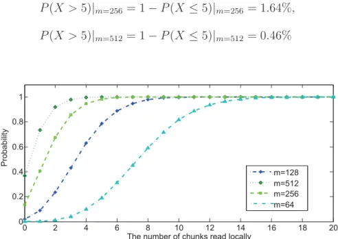
Figure 4.1: CDF of the number of chunks read locally. . . 41

Figure 4.2: A bipartite matching example of processes and chunk files. . . 44

Figure 4.3: The matching-based process-to-file configuration for Single-Data Access . . . 45

Figure 4.4: The process-to-data matching example for Multi-data Assignment. . . 47

Figure 4.5: Access data from HDFS w/o Opass. . . 51

Figure 4.6: Access data from HDFS with Opass. . . 52

Figure 4.7: I/O time on a 64-node cluster. . . 52

Figure 4.8: Access patterns on HDFS w/o Opass. . . 53

Figure 4.9: Access patterns on HDFS with Opass. . . 53

Figure 4.10:Access patterns On a 64-node cluster. . . 54

Figure 4.11:I/O times of tasks with multiple inputs on a 64-node cluster. . . 55

Figure 4.12:Access patterns of multi-inputs on a 64-node cluster. . . 55

(15)

Figure 5.1: The DL-MPI software architecture. . . 60

Figure 5.2: A simple example for tasks assignment. . . 70

Figure 5.3: The comparison of process times. . . 72

Figure 5.4: The bandwidth comparison with the change of cluster nodes. . . 73

Figure 5.5: The bandwidth comparison with the change of file size . . . 74

Figure 6.1: The workload with the change of the cluster size. . . 80

Figure 6.2: The DataNet meta-data structure overnblock files. . . 82

Figure 6.3: An example of a bipartite graph. . . 86

Figure 6.4: Overall execution comparison. . . 90

Figure 6.5: Size of data over HDFS blocks. . . 91

Figure 6.6: Workload distribution after selection. . . 91

Figure 6.7: The map execution time distribution . . . 92

Figure 6.8: The Moving Average map time(s). . . 92

Figure 6.9: The Word Count map time(s). . . 93

Figure 6.10:The Word Count shuffle time(s). . . 94

Figure 6.11:The Top K Search shuffle time(s). . . 95

(16)

Figure 6.13:Workload distribution. . . 96

Figure 6.14:The accuracy of ElasticMap with respect to different sub-datasets. . . 98

(17)

LIST OF TABLES

Table 3.1: Average read time per I/O operation (s) . . . 37

Table 5.1: Descriptions of data locality API in DL-MPI . . . 63

Table 5.2: CASS cluster configuration . . . 71

Table 6.1: The size information of movies within a block file . . . 81

(18)

CHAPTER 1: INTRODUCTION

The advances in sensing, networking and storage technologies have led to the generation and collection of data at extremely high rates and volumes. For instance, the collective amount of genomic information is rapidly expanding from terabytes to petabytes [4] and doubles every 12 months [18, 80, 69]. Petascale simulations in cosmology [41] and climate(UV-CDAT) [86] com-pute at resolutions ranging into the billions of cells and create terabytes or even exabytes of data for visualization and analysis. Also, large corporations, such as Google, Amazon and Facebook pro-duce and collect terabytes of data with respect to click stream or logs in only a few hours [92, 58].

These large-scale scientific and social data require applications to spend more time than ever on analyzing and visualizing them. Parallel computing techniques [49, 11] speed up the perfor-mance of analysis applications by exploiting the inherent parallelism in data mining/rendering algorithms [23]. Commonly used parallel strategies [23] in data analysis includeindependent

par-allelism, task parallelism, andsingle program, multiple data (SPMD) parallelism, which allow a

set of processes to execute in parallel algorithms on partitions of the dataset. In this dissertation, we refer to each operator on data partitions asa data processing taskandparallel data analysisare referred to as the set of parallel processes running simultaneously to perform the tasks.

Conventionally, in parallel big data computing, multiple processes running on different compute nodes share a global parallel file system. Once a data processing task is scheduled to a process, the data will be transferred from the shared file system to the compute processes. Parallel file systems such as PVFS [73] stripe a dataset into many equal pieces and spread them across the storage as shown in Figure 1.1. While such an equal-stripping strategy can allow the storage nodes to serve data requests in a relatively balanced fashion, the process of decoupling parallel storage with computation involves a great deal of data movement over the network. Therefore, the large

(19)

amounts of data movement over the shared network could incur an extra overhead during parallel execution in today’s big data era, especially for the iterative data analysis, which involves moving data from storage to processes repeatedly.

Figure 1.1: File-stripingdata layout in parallel file systems (PVFS).

Distributed file systems [37, 21], such as GFS, HDFS, QFS or Ceph, could be directly deployed on the disks of cluster nodes [38] to reduce data movement. When storing a dataset, distributed file systems will usually divide the data into smaller chunk/block files and randomly distribute them with several identical copies (for the sake of reliability). When retrieving data from HDFS, a client process will first attempt to read the data from the disk that it is running on, referred to as data locality access. If the required data is not on the local disk, the process will then read from another node that contains the required data. Such a architecture of co-locating computation & stoarge exhibits the benefit of local data access in big data processing.

Job or task schedulers in parallel big data applications such as mpiBLAST [56] and ParaView can maximize the usage of computing resources such as memory and CPU by tracking resource consumption/availability for task assignment. However, since these schedulers do not take the distributed I/O resources and global data distribution into consideration, the data requests from

(20)

parallel processes/executors in big data processing will unfortunately be served in an imbalanced fashion on the distributed storage servers. These imbalanced access patterns among storage nodes are caused because a). unlike conventional parallel file system using striping policies to evenly distribute data among storage nodes, data-intensive file systems such as HDFS store each data unit, with several copies based on a relative random policy, which can result in an uneven data distribution among storage nodes; b). based on the data retrieval policy in HDFS, the more data a storage node contains, the higher the probability that the storage node could be selected to serve the data. Therefore, on the nodes serving multiple chunk files, the data requests from different processes/executors will compete for shared resources such as hard disk headandnetwork band-width. Because of this, the makespan of the entire program could be significantly prolonged and the overall I/O performance will degrade.

In general, parallel data analyses impose several challenges on today’s big data processing system and demands additional functionality as discussed below.

• Typical parallel applications such as mpiBLAST run on a HPC system or a cluster with many parallel processes, which execute the same computational algorithm but process different portions of the datasets. The parallel programming model for these applications is the MPI programming model, in which the shared dataset is stored in a network-accessible storage system like NFS, PVFS [73], or Lustre [75], and transferred to a parallel MPI process during execution. This programming model is well-known as the compute-centric model. Thus, the fundamental challenge of running parallel application on HDFS includes the implementation of the co-located compute and storage properties of MPI-based programs, which usually do not take the physical location of data into account during task assignment; and the incom-patibility of conventional I/O interfaces, such as MPI File read(), and HDFS I/O, such as hdfsRead().

(21)

• Data requests from script-based or MPI-based applications such as Paraview [12] usually assign data processing tasks to parallel processes during initialization. These processes can simultaneously issue a large number of data read requests to file systems [78, 23, 98]. With the data stored in HDFS, processes will read their data from their local disk if the required data is on the corresponding disk, or from another remote nodes that contain the required data. However, the data distribution/accesses strategies in HDFS could cause parallel data requests to be served in an imbalanced fashion and thus degrade the I/O performance. In general, the main challenge associated with imbalance issues is finding an assignment of processes to tasks, such that the maximum amount of data can be accessed in a balanced fashion, while also adhering to the constraints of data distribution in HDFS and the load balance requirements of each parallel process/executor. This is complicated by the fact that, a) Parallel processes/executors usually need to be assigned an equal number of tasks so as to maximize the utilization of resources. b) Data in HDFS is not evenly distributed on the cluster nodes, which implies that some processes have more local data than others. c) If an application were to require multiple data inputs, the inputs needed by a task may be stored on multiple nodes.

• Sub-dataset analyses are the process of analyzing specific sub-datasets, e.g, events or topics, to ensure system security and gain business intelligence [57]. A large dataset may contain millions or billions of sub-datasets such as advertisement clicks or event-based log data [9, 5, 33]. The content of a single sub-dataset can be stored in different data partitions, e.g, HDFS blocks, and each block usually contains many sub-datasets. Since sub-dataset analysis programs do not have the knowledge of sub-datasets distribution over HDFS blocks, i.e. the data size of the sub-dataset contained by each block, the sub-dataset filtration or sampling in big data processing will unfortunately result in animbalanced execution in parallel sub-dataset analysis. One main challenge to solve this problem is that collecting and storing the

(22)

meta-data pertaining to the distribution of millions or billions of sub-datasets could incur a substantial cost in memory and CPU cycles.

In order to address the above challenges, we firstly propose a scalable locality-aware middleware (SLAM), which allows scientific analysis applications to benefit from data-locality exploitation with the use of HDFS, while also maintaining the flexibility and efficiency of the MPI program-ming model. SLAM aims to enable parallel processes to achieve high I/O performance in the environment of data-intensive computing and it consists of three components: (1) a data-centric scheduler (DC-scheduler), which transforms a compute-centric mapping into a data-centric one so that a computational process always accesses data from a local or nearby computation node, (2) a data location-aware monitor to support the DC-scheduler by obtaining the physical data distribu-tion in the underlying file system, and (3) a virtual I/O transladistribu-tion layer to enable computadistribu-tional processes to execute conventional I/O operations on distributed file systems. SLAM can benefit not only parallel programs that call our DC-scheduler to optimize data access during development, but also existing programs in which the original process-to-file assignments could be intercepted and re-assigned so as to achieve maximum efficiency on a parallel system.

Secondly, we present a systematic analysis for parallel data imbalanced read on distribution file systems. Based on the analysis, we propose novel matching-based algorithms for parallel big data processing, which assist parallel applications with the assignment of data tasks such that the dis-tributed I/O resources can be maximally utilized as well as to balance the distribution of covariates in datasets and application demands. To achieve this, we retrieve the data layout information for data analysis programs from the underlying distributed file system and model the assignment of processes/executors to data as a one-to-many matching in a Bipartite Matching Graph. We then compute a solution for the matching graph that enables parallel data requests to be served on HDFS in a balanced fashion.

(23)

Thirdly, we propose a novel method to optimize sub-dataset analysis over distributed storage sys-tems referred to as DataNet. DataNet aims to achieve distribution-aware and workload-balanced computing and consists of the following three parts: (1) we propose an efficient algorithm with linear complexity to obtain the meta-data of sub-dataset distributions, (2) we design an elastic storage structure called ElasticMap based on the HashMap and BloomFilter techniques to store the meta-data and (3) we employ a distribution-aware algorithm for sub-dataset applications to achieve a workload-balance in parallel execution. Our proposed method can benefit different sub-dataset analyses with various computational requirements.

(24)

CHAPTER 2: BACKGROUND

In this chapter, we present the workflow of existing parallel applications in scientific analysis and visualization. Specifically, we use two well-known applications to demonstrate how parallel processes access their needed data for analysis and visualization. We also discuss how parallel applications can access data from distributed file systems, e.g, HDFS. We then briefly describe challenges associated with parallel data access on the file systems.

2.1 Scientific Analysis and Visualization Applications

In computational biology, genomic sequencing tools are used to compare given query sequences against database to characterize new sequences and study their effects. There are many dif-ferent alignment algorithms in this field, such as Needleman-Wunsch [66], FASTA [71], and BLAST [13]. Among them, the BLAST family of algorithms is the most widely used in the study of biological and biomedical research. It compares a query sequence with database sequences via a two-phased heuristic-based alignment algorithm. At present, BLAST is a standard defined by the National Center for Biotechnology Information (NCBI).

mpiBLAST [31] is a parallel implementation of NCBI BLAST. As shown in Figure 2.1, mpi-BLAST organizes all parallel processes into one master process and many worker processes. Be-fore performing an actual search, the raw sequence database is formatted into many fragments and stored in a shared network file system with the support of MPI or POSIX I/O operations. mpiBLAST follows a compute-centric model and moves the requested database fragments to the corresponding compute processes. By default, the master process accepts gene sequence search jobs from clients and generates task assignments according to the database fragments, and

(25)

mpi-BLAST workers load database fragments from a globally accessible file system over a network and perform the BLAST task according to the master scheduling. To search through a large database, the I/O cost, which takes place before the real BLAST execution, takes a significant amount of time.

Client

Master

Output file BLAST job submitted

Result merge Data load BLAST

Shared storage

Workers

Network

Figure 2.1: The default mpiBLAST framework: mpiBLAST workers load database fragments from a globally accessible file system over a network and perform BLAST task according to the master scheduling.

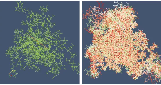
ParaView [12] is an open-source, multi-platform application for the visualization and analysis of scientific datasets. ParaView has three main logical components: data server, render server, and client. The data server reads in files from shared storage and processes data through the pipeline to the render server, which renders this processed data to present the results to the client. The data server can exploit data parallelism by partitioning the data and assigning each data server process a part of the dataset to analyze. By splitting the data, ParaView is able to run data processing tasks in parallel. Figure 2.2 demonstrates an example of parallel visualization for a Protein Dataset.

Current MPI based visualization applications adopt a compute-centric scheduling in which each data server process is assigned tasks according to their MPI ranks. Once a data processing task is scheduled to a data server process, the data will be transferred from a shared storage system to the compute node. Since parallel file systems such as PVFS or Lustre, are usually deployed on storage nodes and data server processes are deployed on compute nodes, this compute-centric model involves a significant amount of data movement for big data problems and becomes a major

(26)

stumbling block to high performance and scalability.

Figure 2.2: A protein dataset is partitioned across multiple parallel processes; the left figure is the sub dataset rendering picture, while the right one is the composite picture of a whole dataset.

2.2 The Hadoop File System and the I/O Interfaces

The Hadoop Distributed File System (HDFS) is an open source implementation of the Google File System (GFS), specifically for the use of MapReduce style workloads. The idea behind the MapReduce framework is that it is faster and more efficient to send the compute executables to the stored data to be processed in-situ rather than to pull the data needed from storage. While HDFS can allow analysis programs to benefit from data locality computation, there are several limitations to running MPI-based analysis applications on HDFS. Firstly, current MPI-based parallel appli-cations are mainly developed with the MPI model, which employs either MPI-I/O or POSIX-I/O to run on a network file system or a network-attached parallel file system. However, HDFS has its own I/O interfaces, which are different from traditional MPI-I/O and POSIX-I/O. Moreover,

(27)

methods to output results, while HDFS only supports “append” write.

2.3 Problems of Runing Parallel Applications On HDFS

Parallel applications such Paraview [12] usually assign data processing tasks to parallel processes during initialization. These processes can simultaneously issue a large number of data read requests to file systems due to the synchronization requirements of parallel processes [78, 23]. Compared to distributed computing applications such as MapReduce programs, parallel applications generally require more precise synchronization and thus a greater number of burst read requests[78, 12, 23, 98]. We specifically discuss two parallel data access challenges in parallel data analysis.

chunk

₁

chunk

₃

... ...

Node 0

chunk

2

chunk

₄

... ...

Node 1

chunk

3

chunk

₁

... ...

Node 2

chunk

1

... ...

Node 3

chunk

₅

P

1

(c

1

,c

2

)

P

2

(c

3

,c

4

)

P

3

(c

5

,c

6

)

P

4

(c

7

,c

8

)

Figure 2.3: The contention of parallel data requests on replica-based data storage.

Parallel Single-Data Access: Most applications based onSPMD or independent parallelism

em-ploy static data assignment methods, which partition input data into independent operators/tasks, with each process working on different data partitions. A typical example is Paraview [12]. Par-aview employs data servers to read files from storage. To process a large dataset, the data servers, running in parallel, read a meta-file, which lists a series of data files. Then, each data server will

(28)

compute their own part of the data assignment according to the number of data files, number of server parallel processes, and their own process rank. For instance, the indices of files assigned to a processiare in the interval:

h

i×_##_{of process}of f iles ,(i+ 1)× _##_{of process}of f iles

The processes read the data in parallel and process data through the pipeline to be rendered. With the data stored in HDFS, a process will read the data from its local disk if its required data is on that disk, or from another remote node that contains the required data. Unfortunately, such a read strategy in HDFS in combination with data assignment methods from applications can cause some cluster nodes to serve more data requests than others. For the example shown in Figure 2.3, three processes can read three data chunks from Node 0 and no process will read data from Node 1, resulting in a lower parallelism utilization of cluster nodes/disks.

dataset of human dataset of mice

dataset of chimpanz.

... inputs of task-0 inputs of task-1

Figure 2.4: An example of parallel tasks with multiple parallel data inputs.

Parallel Multi-Data Access: In certain situations, a single task could have multiple datasets as

input e.g. when the data are categorized into different subsets, such as with the gene datasets of species [42]. For instance, to compare the genome sequences of humans, mice and chimpanzees,

(29)

on different cluster nodes and, without consideration of data distribution and access policy of HDFS, their data requests could cause some storage nodes to suffer a contention, thus degrading the execution performance.

(30)

CHAPTER 3: SCALABLE LOCALITY-AWARE MIDDLEWARE

As data repositories expand exponentially with time and scientific applications become ever more data intensive as well as computationally intensive, a new problem arises in regards to the trans-mission and analysis of data in a computationally efficient manner. Programs running on large-scale clusters in parallel suffer from potentially long I/O latency resulting from non-negligible data movement, especially in commodity clusters with Gigabit Ethernet. As we discussed, scientific analysis applications could significantly benefit from local data access in a distributed fashion with the use of hadoop file system.

In this chapter, we propose a middleware called “SLAM”, which allow scientific analysis pro-grams to benefit from data locality exploitation in HDFS, while also exploiting the flexibility and efficiency of the MPI programming model. Since the data are often distributed in advance within HDFS, the default task assignment, without considering data distribution, may not allow parallel processes to fully benefit the local data access. Thus, we need to intercept the original task schedul-ing and re-assign the tasks to parallel process so as to achieve the maximum efficiency of a parallel system, including a high degree of data locality and load balance. Also, we need to solve the I/O incompatibility issue, such that the data stored in the HDFS can be accessed through conventional parallel I/O methods, e.g, MPI-I/O or POSIX I/O.

SLAM implements a fragment location monitor, which collects an unassigned fragment list at all participating nodes. To achieve this, the monitor needs to make connections to the HDFS NameN-ode using libHDFS, and request chunk location information by asking NameNNameN-ode (specified by a file name, offset within the file, and length of the request). The NameNode replies with a list of the host DataNodes where the requested chunks are physically stored. Based on this locality information, our proposed scheduler will make informed decisions as to which node will be chosen

(31)

to execute a computation task in order to take advantage of data locality. This could realize local data access and avoids data movement in the network.

Specifically, the SLAM framework for parallel BLAST consists of three major components, a translation I/O layer called SLAM-I/O, a data centric load-balanced scheduler called a DC-scheduler and a fragments location monitor, as illustrated in Figure 3.1. Specifically, the Hadoop Distributed File System (HDFS) is chosen as the underlying storage. SLAM-I/O is implemented as an non-intrusive software component added to existing application codes, such that many successful per-formance tuned parallel algorithms and high perper-formance noncontiguous I/O optimization meth-ods [56, 78, 95] can be directly inherited in SLAM. The DC-scheduler determines which specific data fragment is assigned to each node to process. It aims to minimize the number of fragments pulled over the network. DC-scheduler is incorporated into the runtime of parallel BLAST appli-cations. The fragment location monitor will then be invoked by the DC-scheduler to report the database fragments locations.

DFS head

BLAST job submitted

Fragment location monitor

Client

Hadoop distributed file system Parallel BLAST with DC-scheduler

(NEW)

SLAM-I/O layer(NEW)

Query search request

(b) Software Architecture DFS chunks Cluster DC- scheduler Output file Parallel output SLAM-I/O BLAST

Hadoop distributed file system

(a) SLAM

Figure 3.1: Proposed SLAM for parallel BLAST. (a) The DC-scheduler employs a “Fragment Location Monitor” to snoop the fragments location and dispatches unassigned fragments to com-putation processes such that each process could read the fragments locally,i.e., reading chunks in HDFS via SLAM-I/O. (b) The SLAM software architecture. Two new modules are used to as-sist parallel BLAST in accessing the distributed file system and intelligently read fragments with awareness of data locality.

(32)

appro-priate compute nodes, namely, moves computation to data. Through SLAM-I/O, MPI processes can directly access fragments treated as chunks in HDFS from the local hard drive, which is part of the entire HDFS storage.

3.1 SLAM-I/O: A Translation Layer

Current scientific parallel applications are mainly developed with the MPI model, which employs either MPI-I/O or POSIX-I/O to run on a network file system or a network-attached parallel file system. SLAM uses HDFS to replace these file systems, and therefore entails handling the I/O compatibility issues between MPI-based programs and HDFS.

More specifically, scientific parallel applications access files through MPI-I/O or POSIX-I/O inter-faces, which are supported by local UNIX file systems or parallel file systems. These I/O methods are different from the I/O operations in HDFS. For example, HDFS uses a client-server model, in which servers manage metadata while clients request data from servers. These compatibility issues make scientific parallel applications unable to run on HDFS.

To solve the problem, we implement a translation layer—SLAM-I/O to handle the incompatible I/O semantics. The basic idea is to transparently transform high-level I/O operations of parallel applications to standard HDFS I/O calls. We elaborate how I/O works as follows. SLAM-I/O first connects to the HDFS server using hdfsConnect() and mounts HDFS as a local directory at the corresponding compute node. Hence each cluster node works as one client to HDFS. Any I/O operations of parallel applications that work in the mounted directory are intercepted by the layer and redirected to HDFS. Finally, the corresponding hdfs I/O calls are triggered to execute specific I/O functionse.g.open /read /write /close.

(33)

usually produce distributed results and may allow every engaged process write to disjoint ranges in a shared file. For instance, mpiBLAST takes advantage of Independent/Collective I/O to optimize the searched output. TheWorkerCollectiveoutput strategy introduced by Lin et. al.[56] realizes a concurrent write semantic, which can be interpreted as “multiple processes write to a single file at the same time”. These concurrent write schemes often work well with parallel file systems or network file systems. However, HDFS only supports appended write, and most importantly, only one process is allowed to open the file for writing at a time (otherwise an open error will occur). To resolve this incompatible I/O semantics issue, we revise “concurrent write to one file” to “concurrent write to multiple files”. We allow every process output their results and the write ranges independently into a physical file in HDFS. Logically, all output files produced for a data processing job are allocated in the same directory. The overall results are retrieved by joining all physical files under the same directory.

In our experimental evaluation, we prototyped SLAM-I/O using FUSE [3], a framework for run-ning stackable file systems in a non-privileged mode. An I/O call from an application to the Hadoop file system is illustrated in Figure 3.2. The Hadoop file system is mounted on all partic-ipating cluster nodes through the SLAM-I/O layer. The I/O operations of mpiBLAST are passed through a virtual file system (VFS), taken over by SLAM-I/O through FUSE and then forwarded to HDFS. HDFS is responsible for the actual data storage management. In regards to concur-rent write, SLAM-I/O automatically inserts a subpath using the same name as the output filename and appends its process ID at the end of the file name. For instance, if a process with id 30

writes into/hdf s/f oo/searchNT result, the actual output file is/hdf s/f oo/serachNT result/ searchNT result30.

(34)

MPI-I/O, POSIX-I/O

FUSE lib SLAM-I/O

VFS-System call() Kernel FUSE Kernel Module DFS I/O HDFS

Figure 3.2: The I/O call in our prototype. A FUSE kernel module redirects file system calls from parallel I/O to SLAM-I/O and SLAM-I/O wrappers HDFS clients and translates the I/o call to DFS I/O.

3.2 A Data Centric Scheduler

As discussed, the key to realizing scalability and high-performance in big data scientific applica-tions is to achieve data locality and load balance. However, there exists several heterogeneity issues that could potentially result in load imbalance. For instance, in parallel gene data processing, the global database is formatted into many fragments. The data processing job is divided into a list of tasks corresponding to the database fragments. On the other hand, the HDFS random chunk place-ment algorithm may distribute database fragplace-ments unevenly within the cluster, leaving some nodes with more data than others. In addition, the execution time of a specific BLAST task could vary greatly and is difficult to predict according to the input data size and different computing capacities per node [34, 56].

We implement a fragment location monitor as a background daemon to report updated unassigned fragment statuses to the DC-scheduler. At any point in time, the DC-scheduler always tries to launch alocal taskof the requesting process, that is, a task with its corresponding fragment avail-able on the node issued by the requesting process. There exists a good chance of achieving a high degree of data locality, as each fragment has three physical copies in HDFS, namely, there are three

(35)

different node candidates available for scheduling.

Upon an incoming data processing job, the DC-scheduler invokes the location monitor to report the physical locations of all target fragments. If a process from a specific node requests a task, the scheduler assigns a task to the process using the following procedure. First, if there exists local tasks on the requesting node, the scheduler will evaluate which local task should be assigned to the requesting process in order to make other parallel processes achieve locality as much as possible (details will be provided later). Second, if there does not exist any local task on the node, the scheduler will assign a task to the requesting process by comparing all unassigned tasks in order to make other parallel processes achieve locality. The node will then pull the corresponding fragment over the network.

Algorithm 3.2.1Data centric load-balanced Scheduler Algorithm

1: LetF ={f1, f2, ..., fm}be the set of tasks

2: LetFi be the set of unassigned local tasks located on nodei Steps:

3: InitializeF for a data processing job

4: InvokeLocation monitorand initializeFi for each nodei

5: while|F| 6= 0do

6: ifa worker process on nodeirequests a taskthen

7: if |Fi| 6= 0 then

8: Findfx ∈Fi such that

9: x= argmax

x

( min Fk∋fx,k6=i

(|Fk|))

10: Assignfx to the requesting process on nodei

11: else

12: Findfx ∈F such that

13: x= argmax

x

( min Fk∋fx,k6=i

(|Fk|))

14: Assignfx to the requesting process on nodei

15: end if 16: RemovefxfromF 17: for allFks.t. fx ∈Fkdo 18: RemovefxfromFk 19: end for 20: end if 21: end while

(36)

The scheduler is detailed in Algorithm 1. The input data processing job consists of a list F of individual tasks, each associated with a distinct fragment. While the tasks list, F, is not empty, parallel processes report to the scheduler for assignments. Upon receiving a task request from an process on Nodei, the scheduler determines a task for the process as follows:

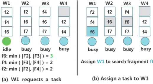
• 1. If Node i has some local tasks, then the local task x that could make the number of unassigned local tasks on all other nodes as balanced as possible will be assigned to the requesting process. Figure 3.3 illustrates an example to demonstrate how this choice is made. In the example, there are4parallel processes running on4nodes, whereW1requests a task from its unassigned local tasks F1 =< f2, f4, f6 >. For each task fx inF1, we compute

the minimum number of unassigned tasks among all other nodes containingfx’s associated fragment. For example, the taskf2is local toF2andF4, so we computemin(|F2|,|F4|) = 2.

We assign the task with the largest such value to the idle process, which isf6in the example.

After the assignment, the number of unassigned local tasks for node W2, W3 and W4

become2,2,2, as shown in Figure 3.3 (b).

• 2. If nodeidoes not contain any unassigned local tasks, the scheduler will perform the above calculation for all unassigned tasks inF and assign the task with the largestminvalue to the requesting process, which needs to pull data over network.

Since mpiBLAST adopts a master-slave architecture, the DC-scheduler could be directly incorpo-rated into the master process, which performs dynamic scheduling according which nodes are idle at any given time. For such scheduling problems, minimizing the longest execution time is known to be NP-complete [35] when the number of nodes is greater than2, even for the case that all tasks are executed locally. However we will show that for this case, the execution time of our solution is at most two times that of the optimal solution.

(37)

W1 W2 W3 W4 idle f6: min ( |F2|, |F3| ) =3 f4: min ( |F3|, |F4| ) = 2 f2: min ( |F2|, |F4| ) = 2 busy busy busy (b) Assign a task to W1 (a) W1 requests a task

AssignW1to search fragmentf6

f2 f4 f6 f2 f6 f7 f4 f6 f7 f2 f4 W1 W2 W3 W4 busy busy busy f2 f4 f6 f2 f6 f7 f4 f6 f7 f2 f4 busy

Figure 3.3: A simple example of the DC-scheduler receiving the task request of the process (W1). The scheduler finds the unassigned local tasks ofW1(f2,f4andf6in this example). The taskf6

will be assigned toW1since the minimum unassigned task value is3onW2andW3, which also hasf6as a local task. After assigningf6toW1, the number of unassigned local tasks ofW1–4is

2.

Suppose there are m = |F|tasks with actual execution times of t1, t2, ..., tm onn = |W| nodes. We useT∗ _{to denote the maximum execution time of a node in the optimal solution. Notice that} T∗_{cannot be smaller than the maximum execution time of a single task. This observation gives us}

a lowerbound forT∗_:

T∗ ≥ max

1≤k≤m(tk) (3.1)

LetT be the maximum execution time of a node in a solution given by our algorithm. Without loss of generality, we assume that the last completed taskfnis scheduled on noden. Letsfndenote the start time of taskfnon noden, soT =sfn +tn.

(38)

will be assigned to some nodes earlier. Therefore we haveT∗ _≥ _s

fn. Because T

∗ _≥ _max 1≤k≤m(tk), we haveT∗ _≥_t

n. This gives us the desired approximation bound:

T =sfn+tn≤2T

∗ _(3.2)

The scheduling problem is even much harder when we take the location variable into consideration. However, we will conduct real experiments to examine its locality and parallel execution in Section 4.

3.3 ParaView with SLAM

As we discussed, ParaView could suffer from non-negligible data movement and network con-tention, resulting in serious performance degradation. As with parallel BLAST, ParaView could benefit from local data access in a distributed fashion. Allowing ParaView to achieve data locality computation requires the replacement of the data partition scheduling in the ParaView reader mod-ules on each data server processes, which ingest data from files according to the task assignment.

Currently, there are a large number of data readers with support for various scientific file formats. Specifically, examples of parallel data readers [79] are Partitioned Legacy VTK Reader, Multi-Block Data Reader, Hierarchical Box Data reader, Partitioned Polydata Reader, etc. To process a data set, the data servers, running in parallel, will call the reader to read a meta-file, which points to a series of data files. Then each data server will compute their own part of the data assignment according to the number of data files, number of parallel servers, and the their own server rank. Data servers will read the data in parallel from the shared storage and then filter/render.

(39)

as-signment and use our proposed DC-scheduler to assign tasks for each data server at run time. Specifically, the SLAM framework for ParaView also includes three components, the translation layer — SLAM-I/O, the DC-scheduler and the fragments location monitor, as illustrated in Fig-ure 3.4. The DC-scheduler determines which specific data fragment is assigned to each data server process. To get the physical location of the target data sets, the Location Monitor is invoked by the DC-scheduler to report the data fragments locations. Through SLAM-I/O, the data server pro-cesses can directly access data, treated as chunks in HDFS, from the local hard drive, which is part of the entire HDFS storage.

SLAM -I/O Location Monitor HDFS DC-Scheduler (process id)

Figure 3.4: Proposed SLAM for ParaView. The DC-scheduler assign data processing tasks to MPI processes such that each MPI process could read the needed data locally,i.e., reading chunks in HDFS via SLAM-I/O.

Our proposed DC-scheduler algorithm in Section 3.3 is very suitable for the applications with dynamic scheduling algorithms, such as mpiBLAST, in which scheduling is determined by which nodes are idle at any given time. However, since the data assignment in ParaView uses a static data partitioning method, the work allocation is determined beforehand; no process works as a central scheduler. For this kind of scheduling, we adopt a round-robin request order for all data server in Step 8 of Algorithm 3.2.1. Until the setF is empty, the the data server process with a specificpid

can get all the data pieces assigned to it. Then the data servers will read the data in parallel and then filter/render.

(40)

3.4 Specific HDFS Considerations

HDFS employs some default data placement policies. A few considerations should be taken into account when we choose HDFS as the shared storage. First, each individual fragment file size should not exceed the configured chunk size, otherwise the file will be broken up into multiple chunks with each chunk replicated independently of other related chunks. If only a fraction of the specific fragment can be accessed locally, other parts must be pulled over the network. Con-sequently, the locality benefit is lost. As a result, we should keep the file size of each database fragment smaller than the chunk size when formatting the data set. Second, for parallel BLAST, when applying the database format method, each fragment includes seven related files, six of which are smaller files and one is bigger. The hadoop Archivemethod should be applied to ensure that these seven files are stored together during a formatted execution.

3.5 Experiments and Analysis

3.5.1 Experimental Setup

We conducted comprehensive testing on our proposed middleware SLAM on both Marmot and CASS clusters with different storage systems. Marmot is a cluster of PRObE on-site project and housed at CMU in Pittsburgh. The system has 128 nodes / 256 cores and each node in the clus-ter has dual 1.6GHz AMD Opclus-teron processors, 16GB of memory, Gigabit Ethernet, and a 2TB Western Digital SATA disk drive. CASSconsists of46nodes on two racks, one rack including15

compute nodes and one head node and the other rack containing30compute nodes. Each node is equipped with dual 2.33GHz Xeon Dual Core processors, 4GB of memory, Gigabit Ethernet and a 500GB SATA hard drive.

(41)

In both clusters, MPICH [1.4.1]is installed as parallel programming framework on all compute nodes running CENTOS55-64 with kernel 2.6. We chose Hadoop0.20.203as the distributed file system, which is configured as follows: one node for the NameNode/JobTracker, one node for the secondary NameNode, and other nodes as the DataNode/TaskTracker. In addition, we chose two conventional file systems as our baseline file systems for a comprehensive test. We run experiments on NFS as the developers of mpiBLAST use NFS as shared storage [56]. We also installed PVFS2 version[2.8.2]with default setting on the cluster nodes: one node as the metadata server for PVFS2, and other nodes as the I/O servers (similar to HDFS).

3.5.2 Evaluating Parallel BLAST with SLAM

To make a fair comparison with the open source parallel BLAST, we deploy mpiBLAST [1.6.0]

on all nodes in the clusters that support the techniques of query prefetch and computation & I/O coordination methods that would coordinate dynamic load balancing of computation and high per-formance noncontiguous I/O. Equipped with our SLAM-I/O layer at each cluster node, HDFS can be mounted as a local directory and used as shared storage for parallel BLAST. The BLAST itself can run on HDFS without recompilation. We implement the fragment location monitor and the DC-scheduler and incorporate both modules into the mpiBLAST master scheduler to exploit data locality as shown in Figure 3.1. When running parallel BLAST, we let the scheduler process run on the node on which the NameNode is configured, and parallel processes run on the DataNodes for the sake of locality.

We select the nucleotide sequence database nt as our experimental database. The nt database contains the GenBank, EMB L, D, and PDB sequences. At the time when we performed our experiments, thentdatabase contained 17,611,492 sequences with a total raw size of about45GB. The input queries to search against thentdatabase are randomly chosen fromntand revised, which

(42)

guarantees that we find some close matches in the database.

When running mpiBLAST on the cluster with directly attached disks, users usually runfastasplitn

andformatdbonce and reuse the formatted database fragments. To deliver database fragments, we

use a dynamic copying method such that the node will copy and cache a data fragment only when a search task to the fragment is scheduled on the node. These cached fragments are reused for subsequent sequences searches. mpiBLAST is configured with two conventional file systems— NFS and PVFS2 and both work as baselines. SLAM employs HDFS as a distributed storage. Therefore, there is no need for gathering a fragment over network from multi data nodes as PVFS does, and we do not cache fragments in local disks either.

We studied how SLAM could improve the performance for parallel BLAST. We scaled up the num-ber of data nodes in the cluster and compared the performance with three host file system configu-rations: NFS, PVFS2 and HDFS, respectively. For clarity, we labeled them as NFS-based, PVFS-based and SLAM-PVFS-based BLAST. During the experiments, we mount NFS, HDFS and PVFS2 as the local file systems at each node if a BLAST process is running on that node. We used the same input query in all running cases and fix the query size to50KB with 100 sequences, which generated a consistent output result of around 5.8MB. Thent database was partitioned into 200

fragments.

3.5.2.1 Results from an Marmot Cluster

The experimental results collected from Marmot are illustrated in Figures 3.5, 3.6, 3.7 and 3.8.

When running parallel BLAST on a 108-node configuration system, we found the total program ex-ecution time with NFS-based, PVFS-based and SLAM-based BLAST to be 589.4, 379.7 and 240.1 seconds, respectively. We calculate the performance gain with Equation 3.3, whereTSLAM-based

(43)

de-notes the overall execution time of parallel BLAST based on SLAM andTNFS/PVFS-basedis the overall

execution time of mpiBLAST based on NFS or PVFS.

improvement = 1− TSLAM-based TNFS/PVFS-based . (3.3) 0% 10% 20% 30% 40% 50% 60% 70% 4 8 16 32 64 96 108 Im p ro v e m e n t NumberofNodes

Improvement

in

Use

of

SLAM

NFSͲbased PVFSͲbased

Figure 3.5: The performance gain of mpiBLAST execution time when searching the ntdatabase in use of SLAM as compared to NFS-based and PVFS-based.

As seen from Figure 3.5, we conclude that SLAM-based BLAST could reduce overall execution latency by 15% to 30% for small-sized clusters with less than 32 nodes as compared to NFS-based BLAST. Given an increasing cluster size, SLAM reduces overall execution time by a greater percentage, reaching 60% for a 108-node cluster setting. This indicates that the NFS-based setting is not scaling well. In comparison to PVFS-based BLAST, SLAM runs consistently faster by about 40% for all cluster settings.

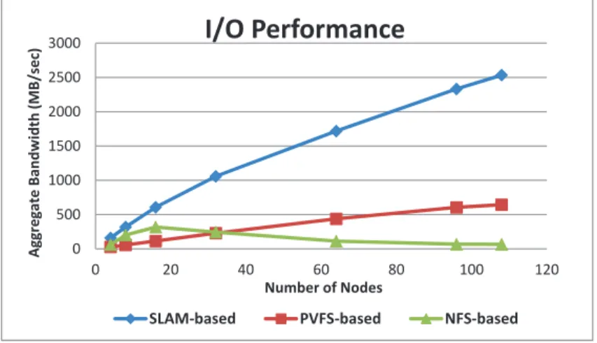
To test scalability we collected results of aggregated I/O bandwidth for an increasing number of nodes as illustrated in Figure 3.6. We find that in SLAM the I/O bandwidth greatly increases as the number of nodes increases, proving it to be a scalable system. However, the NFS and PVFS based BLAST schemes have a considerably lower overall bandwidth, and as the number of nodes

(44)

in the other file systems increases, they do not achieve the same bandwidth increase from more nodes. This indicates a large data movement overhead exists in NFS and PVFS that hinder their scalability. Ͳ Ͳ 0 500 1000 1500 2000 2500 3000 0 20 40 60 80 100 120 A g g re g a te B a n d w id th (M B /s e c) NumberofNodes

I/O

Performance

SLAMͲbased PVFSͲbased NFSͲbased

Figure 3.6: The input bandwidth comparison of NFS-based, PVFS-based and SLAM-based BLAST scheme. The key observation is that SLAM scales linearly well for search workloads.

Ͳ

Ͳ Ͳ Ͳ 0 500 1000 1500 2000 2500 3000 4 8 16 32 64 96 108 T o ta l T im e ( se co n d ) NumberofNodes

I/O

Latency

SLAMͲbased PVFSͲbased

Figure 3.7: The I/O latency comparison of PVFS-based and SLAM-based BLAST schemes on the ntdatabase with an increasing number of nodes.

(45)

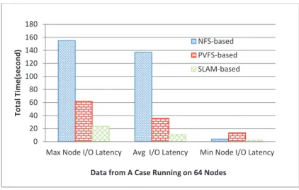
illustrated in Figure 3.7. We find that the total I/O latency of PVFS based BLAST is close to 2,000 seconds for clusters of 32 nodes and increases thereafter. On the other hand, SLAM achieves a much lower I/O latency than PVFS with latency times being a quarter of that of PVFS for clusters up to 64 nodes, and a fifth for larger networks. Figure 3.8 shows the particular case of I/O latency times on a 64 node cluster using SLAM, PVFS, and NFS. Three latency figures are presented for each file system: maximum node latency, minimum node latency, and average latency. SLAM excels in having low latency times in all three tests while maintaining a small difference in I/O time between the fastest and slowest node, and ultimately achieves the lowest latency times of all three systems. NFS and PVFS suffer from an imbalance in node latency and on average are considerably slower than SLAM.

Ͳ

Ͳ Ͳ Ͳ 0 20 40 60 80 100 120 140 160 180

MaxNodeI/OLatency AvgI/OLatency MinNodeI/OLatency

T o ta l T im e (s e co n d )

DatafromACaseRunningon64Nodes

NFSͲbased PVFSͲbased SLAMͲbased

Figure 3.8: The max and min node I/O time comparison of NFS-based, PVFS-based and SLAM-based BLAST on the ntwith varying number of nodes.

3.5.2.2 Results from a CASS Cluster

For a comprehensive testing, we performed similar experiments at an on-site CASS cluster. We distinguish the average actual BLAST times from I/O latency to gain some insights about

(46)

scalabil-ity. Ͳ

Ͳ Ͳ Ͳ 0 100 200 300 400 500 600 700 800 0 10 20 30 40 A v e ra g e B LA S T T im e (s ) NumberofNodes

Actual

BLAST

Comparison

NFSͲbased PVFSͲbased SLAMͲbased

Figure 3.9: The actual BLAST time comparison of NFS-based, PVFS-based and SLAM-based BLAST programs on the ntdatabase with different number of nodes.

0 100 200 300 400 500 600 700 2 6 10 14 18 22 26 30 34 38 NFSͲbased PVFSͲbased SLAMͲbased Number of Nodes A v er a g e T im e (s )

Averge I/O Latency Comparison

Figure 3.10: The average I/O time of NFS-based, PVFS-based and SLAM-based BLAST on the ntdatabase with different number of nodes.

Figure 3.9 illustrates the average actual BLAST computation times (excluding I/O latency) in an increasing cluster size. We find that the average actual BLAST time in Figure 3.9 decreases

(47)

sharply as the number of nodes grow. The three systems that we tested obtained comparable BLAST performances. This supports our conjecture as SLAM only targets I/O rather than real BLAST computation. Different file system configurations—NFS, PVFS, and HDFS account for the differences among three BLAST programs. Figure 3.10 illustrates the I/O phase of the BLAST workflow. In NSF and PVFS baselines, the average I/O cost remains consistent, at around 100 seconds, after cluster size exceeds 15. In contrast, SLAM adopts a scalable HDFS solution, which realizes a decreasing I/O latency along with an increasing number of nodes.

The priority of our DC-scheduler is to achieve data-task locality while adhering to load balance constraints. To explore the effectiveness of the DC-scheduler,(i.e., to what extent search processes are scheduled to access fragments from local disks), Figure 3.11 illustrates one snapshot of the fragments searched on each node and the fragments access by the network. We specifically ran experiments five times to check how much data is moved through the network in a 30-node setting, and track down a total number of fragments 150, 180, 200, 210, 240 respectively. As seen from the Figure 3.11, most nodes search a comparable number of fragments locally. More than 95% of the data fragments are read from local storage.

We also run mpiBLAST on HDFS using only our I/O translation layer (without the locality sched-uler) and found that the performance is only slightly better than that of PVFS-based BLAST. This is because BLAST processes need to read data remotely without the coordination of data locality scheduler. We will show the detail comparison in the next Subsection.

3.5.2.3 Comparing with Hadoop-based BLAST

We only show a simple comparison with Hadoop-based Blast from Marmot, as such a comparison may be unfair since the efficiency, while being the design goal of MPI, is not the key feature of the MapReduce programming model.

(48)

0 20 40 60 80 100 120 140 160 180 200 0 5 10 15 20 25 30 F ra g m e n t ID NodeID

DC

Ͳ

Scheduler

Performance

Local Access Remote Access

Figure 3.11: Illustration of which data fragments are accessed locally on which node and involved in the search process. The blue triangles represent the data fragments accessed locally during the search, while the red dots represent the fragments accessed remotely.

We chose Hadoop-Blast [7] as the Hadoop-based approach. The database for both programs are ‘nt’ and the input query is same. With a 25-nodes setting on marmot, SLAM-based BLAST takes 568.664 seconds while Hadoop-Blast takes 1427.389 seconds. We run the tests several times, and the SLAM-based BLAST is always more efficient than Hadoop-based BLAST. The reasons could be, 1) the task assignment of Hadoop-Blast relies on the Hadoop Scheduler, which is built on the heartbeat mechanism, 2) the advantages of I/O optimization based on MPI are not adapted by Hadoop-Blast, and 3) the difference in efficiency of Java and C/C++ implementation [81].

3.5.3 Efficiency of SLAM-I/O Layer and HDFS

In the SLAM-based BLAST framework, a translation layer—SLAM-I/O is developed to allow parallel I/O to execute on distributed file systems. In our prototype, we chose FUSE mount to transparently relink these I/O operations to the HDFS I/O interface. Thus, there is a need for

(49)

evaluating the incurred overhead of a FUSE-based implementation.

SLAM-I/O is built through a Virtual File System (VFS). The I/O call needs to go through the kernel of the client operating system. For instance, to read an index file nt.mbf in HDFS, mpiBLAST issues an open() call first through the VFS’s generic system call (sys-open()). Next, the call is translated to hdfsOpenFile(). Finally, the open operation will take effect on HDFS. We conduct experiments to quantify how much overhead the translation layer running for parallel BLAST would incur.

We run the search programs and measured the time it takes to open the 200 formatted fragments. We did two kind of tests. The first directly uses the HDFS library while the other uses the default POSIX I/O, running HDFS file open through our SLAM-I/O layer. For each opened file, we read the first 100 bytes and then close the file. We repeated the experiment several times. We found that the average total time through SLAM-I/O is around 15 seconds. The time through direct HDFS I/O was actually 25 seconds. This may result from the overhead of connecting and disconnecting with hdfsConnect() independently for each file. For the second experiment, we ran a BLAST process on multiple nodes through SLAM-I/O. The average time to open a file in HDFS is around 0.075 seconds, which is negligible compared with the overall data input time and BLAST time. In all, a FUSE based implementation does not introduce non-negligible overhead. Sometimes, SLAM-I/O actually performs better than the libhdfs based hard coding solution.

In the default mpiBLAST, each worker maintains a fragmentation list to track the fragments on its local disk and transfers the metadata information to the master scheduler via message passing. The master uses a fragment distribution class to audit scheduling. In SLAM, the NameNode is instead responsible for the metadata management. At the beginning of a computational workflow, a fragment location monitor retrieves the physical location of all fragments by talking to Hadoop’s NameNode. We evaluated the HDFS overhead by retrieving the physical location of 200 formatted

(50)

fragments. The average time is around 1.20 seconds, which accounts for a very small portion of the overall data input time.

3.5.4 Evaluating ParaView with SLAM

To test the performance of ParaView with SLAM, ParaView 3.14 was installed on all nodes in the cluster. To enable off-screen rendering, ParaView made use of the Mesa 3D graphics library version 7.7.1. The DC-scheduler is implemented with VTK MultiBlock datasets reader for data task assignment. A multi-block dataset is a series of sub datasets, together they represent an assembly of parts or a collection of meshes of different types from a coupled simulation [8].

To deal with MultiBlock datasets, a meta-file with extension “.vtm” or “.vtmb” is read as an index file, which points to a series of VTK XML data files constituting the subsets. The series of data files are either PolyData, ImageData, RectilinearGrid, UnstructuredGrid or StructuredGrid with the extension .vtp, .vti, .vtr, .vtu or .vts. Specifically, our scheduler method is implemented in the vtkXMLCompositeDataReader class and called in the function ReadXMLData(), which assigns the data pieces to each data server after processing the meta-file. Through intercepting the original static data assignment into our DC-scheduler, each data server process can receive the proper task assignment with it’s associated data locally accessible. The data server will then be able to perform the data processing tasks according to the data assignment.

For our test dataset we use the data of a Macromolecular structure that was obtained from a Protein Data Bank [10] containing a repository of atomic coordinates and other information describing proteins and other important biological macromolecules. The processed output of these protein datasets are polygonal images, and ParaView is used to process and display such structures from the datasets. Through ParaView, scientists can also compare different biological datasets by measuring

(51)

each data set as a time step and convert it to a subset of ParaView’s MultiBlock file with extension “.vtu”. Due to the need to download multiple data sets to the test system, we duplicate some datasets with some revisions and save them as new datasets.

It should be noted that the data was written in “binary” mode to allow for the smallest possible amount of time to be spent on parsing the data by the ParaView readers. Additionally, for each rendering, 96 subsets from 960 data sets were selected. As a result, our test set was approximately 40 GB in total size and 3.8 GB per rendering step.

3.5.4.1 Performance Improvement with the Use of SLAM

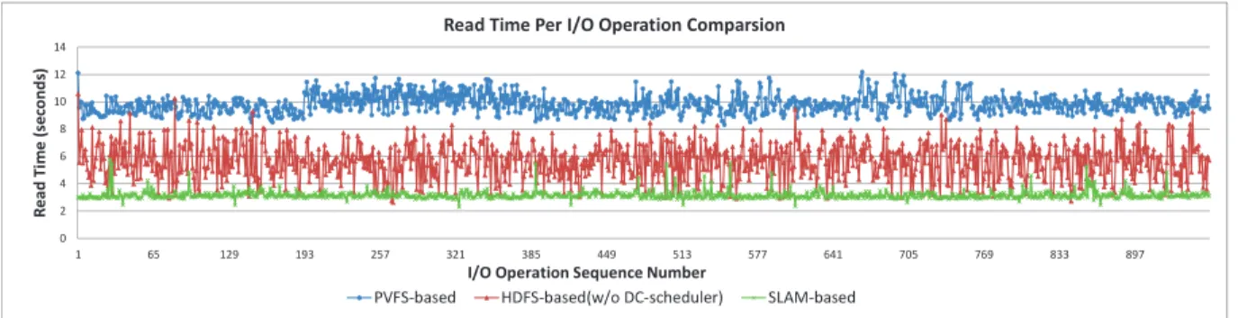
Performance is characterized by two aspects of the ParaView experiment: the overall execution time of the ParaView rendering and the data read time per I/O operation during program execution.

Figure 3.12 illustrates the execution time of a ParaView analysis for an increasing number of nodes with PVFS, HDFS file systems. With a small cluster of 16 nodes, the total time of the ParaView experiment did not greatly differ between the three methods, though there was some advantage to the SLAM based ParaView, which executed in 300 seconds. A 32 node cluster displayed the same attributes with ParaView executing in 200 seconds. At 64 nodes however, the SLAM based ParaView shows it’s strength in large clusters seeing a large reduction in total time when compared with the PVFS and HDFS filesystems being nearly 100 seconds quicker in execution for a total execution time of 110 seconds. In a 96 node cluster, the difference between SLAM and the other filesystems is lessened. However, a great improvement is observed with SLAM based ParaView, which executes in 70 seconds, a reduction of almost 2X over PVFS and HDFS.

Figure 3.12 visualizes the time per process of a ParaView simulation on a 96 node cluster in marmot. With PVFS, data read times are consistently slow due to it’s network loaded datasets and

Research on High-performance and Scalable Data Access in Parallel Big Data Computing

STARS

STARS

Research on High-performance and Scalable Data Access in

Research on High-performance and Scalable Data Access in

Parallel Big Data Computing

Parallel Big Data Computing

ABSTRACT

ACKNOWLEDGMENTS

TABLE OF CONTENTS

LIST OF FIGURES

LIST OF TABLES

CHAPTER 1: INTRODUCTION

CHAPTER 2: BACKGROUND

chunk

chunk

... ...

Node 0

chunk

chunk

... ...

Node 1

chunk

chunk

... ...

Node 2

chunk

... ...

Node 3

chunk

P

(c

,c

)

P

(c

,c

)

P

(c

,c

)

P

(c

,c

)

CHAPTER 3: SCALABLE LOCALITY-AWARE MIDDLEWARE

Improvement

in

Use

of

SLAM

I/O

Performance

I/O

Latency

Actual

BLAST

Comparison

DC

Ͳ

Scheduler

Performance