Functional Graphical Models
Xinghao Qiao
1, Shaojun Guo
∗2, and Gareth M. James
31Department of Statistics, London School of Economics, U.K.
2Institute of Statistics and Big Data, Renmin University of China, P.R. China 3Department of Data Sciences and Operations, University of Southern California, USA
Abstract
Graphical models have attracted increasing attention in recent years, especially in settings involving high dimensional data. In particular Gaussian graphical models are used to model the conditional dependence structure among multiple Gaussian random variables. As a result of its computational efficiency the graphical lasso (glasso) has become one of the most popular approaches for fitting high dimensional graphical mod-els. In this article we extend the graphical models concept to model the conditional dependence structure among p random functions. In this setting, not only is p large, but each function is itself a high dimensional object, posing an additional level of sta-tistical and computational complexity. We develop an extension of the glasso criterion (fglasso), which estimates the functional graphical modelby imposing a block sparsity constraint on the precision matrix, via a group lasso penalty. The fglasso criterion can be optimized using an efficient block coordinate descent algorithm. We establish the concentration inequalities of the estimates, which guarantee the desirable graph sup-port recovery property, i.e. with probability tending to one, the fglasso will correctly identify the true conditional dependence structure. Finally we show that the fglasso ∗Shaojun Guo was partially supported by National Science Foundation of China (NO. 11771447).
significantly outperforms possible competing methods through both simulations and an analysis of a real world EEG data set comparing alcoholic and non-alcoholic patients.
Some key words: Functional data; Graphical models; Functional principal component analysis; Block sparse precision matrix, Block coordinate descent algorithm.
1
Introduction
The graphical model is used to depict the conditional dependence structure amongprandom variables,X= (X1, . . . , Xp)T. Such a network consists ofpnodes, one for each variable, and
a number of edges connecting a subset of the nodes. The edges describe the conditional dependence structure of the p variables, i.e. nodes j and l are connected by an edge if and only if Xj and Xl are correlated, conditional on the other p−2 variables. Recently there
has been a lot of interest in fitting high dimensional graphical models, where pis very large. For Gaussian data, where X follows a multivariate Gaussian distribution, one can show that estimating the edge set is equivalent to identifying the locations of the non-zero elements in the precision matrix, i.e. the inverse covariance matrix of X. Hence, the literature has mainly focused on two approaches for estimating high dimensional Gaussian graphical
models. One type of method, proposed by Meinshausen and Buhlmann (2006), considers
neighbourhood selection. It adopts a lasso (Tibshirani, 1996) or Dantzig selector (Candes and Tao, 2007) type of penalized regression approach whereby each variable is regressed on the other variables, thus identifying the locations of non-zero entries in the precision matrix column by column, see also Peng et al. (2009); Cai et al. (2011); Sun and Zhang (2013). Another method, proposed by Yuan and Lin (2007), optimizes the graphical lasso (glasso) criterion, essentially a Gaussian log likelihood with the addition of a lasso type penalty on the entries of the precision matrix. The glasso has arguably proved the most popular of these two methods, in part because a number of efficient algorithms have been developed to minimize the convex glasso criterion (Friedman et al.,2007;Boyd et al.,2010;Witten et al.,
2011;Mazumder and Hastie,2012a,b). Its theoretical properties have also been well studied (Lam and Fan, 2009; Ravikumar et al., 2011), and several variants and extensions of the glasso have been proposed, see Zhou et al. (2010); Kolar and Xing (2011); Danaher et al.
(2014); Zhu et al.(2014) and the references therein.
In this paper we are interested in estimating a graphical network in a somewhat more complicated setting. Let g1(t), . . . , gp(t) jointly follow from a p-dimensional multivariate
Gaussian process(MGP) wheret ∈ T andT is a closed subset of the real line1. Our goal is to
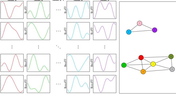
construct afunctional graphical model(FGM) depicting the conditional dependence structure among theseprandom functions. The left panel of Figure 1provides an illustrative example withp= 9 functions, or nodes. We have 100 observations of each function, corresponding to 100 individuals. In other words our data consists of functions,gij(t) wherei= 1, . . . ,100 and
j = 1, . . . ,9. The right panel of Figure 1 illustrates the conditional dependence structure of these functions i.e. the FGM. For example, we observe that the last 3 functions are disconnected from, and hence conditionally independent of, the first 6 functions. We wish to take the observed functions in the left panel and estimate the FGM in the right panel.
Our motivating example is an electroencephalography (EEG) data set taken from an alcoholism study (Zhang et al., 1995; Ingber,1997). The study consists of n= 122 subjects split between an alcoholic group and a control group. Each subject was exposed to either a single stimulus or two stimuli. The resulting EEG activity was recorded at 256 time points over a one second interval using electrodes placed at 64 standard locations on the subject’s scalp. Hence, each observation, or subject, involves p = 64 different functions observed at 256 time points. It is of scientific interest to identify differences in brain EEG activity filtered atα frequency bands (Hayden et al.,2006) between the two groups, so we construct FGM’s for each group and explore the differences. Functional data of this sort can arise in a number
1Here we assume the same time domain, T, for all random functions to simplify the notation, but
our methodological and theoretical results extend naturally to the more general case where each function corresponds to a different time domain.
Node 1 g1 ,1 ( t ) Node 2 g1 ,2 ( t ) ● ● ● Node 3−7 Node 8 g1 ,8 ( t ) Node 9 g1 ,9 ( t ) g2 ,1 ( t ) g2 ,2 ( t ) ● ● ● g2 ,8 ( t ) g2 ,9 ( t ) ● ● ● ● ● ● ● ● ● ● ● ● ● ● ● g99 ,1 ( t ) g99 ,2 ( t ) ● ● ● g99 ,8 ( t ) g99 ,9 ( t ) g100 ,1 ( t ) g100 ,2 ( t ) ● ● ● g100 ,8 ( t ) g100 ,9 ( t ) 1 2 3 4 5 6 7 8 9
Figure 1: The illustrative example. Left: The data, n= 100 observations ofgij(t) for j= 1, . . . ,9
nodes. Right: the true underlying network structure.
of other contexts. For example, rather than recording only a static set of p gene expression levels at a single point in time, it is now becoming common to observe multiple expression levels over time (Storey et al., 2005), so gij(t) would represent the expression level of gene
j for subject i at time t. Alternatively, in a marketing context it is now possible to observe online purchase patterns among a basket of p different products for each of n individual customers over a period of time, so gij(t) might represent the cumulative purchase history
of product j by customer iat time t.
One possible approach to handle this sort of functional data would be to sample the functions over a grid of time points, t1, . . . , tT, estimate T separate networks, and then
either report all T networks or construct a single graphical model by somehow merging the
T networks. However, while conceptually simple, this strategy has several drawbacks. First, the approach is only possible if g1(t), . . . , gp(t) are observed over a common domain t ∈ T,
observed over a relatively sparse set of time points which makes it impossible to create a single set of grid points,t1, . . . , tT, at which the functions can be sampled. Third, one of the main
advantages of a graphical network is its ability to provide a relatively simple representation of the conditional dependence structure. However, simultaneously interpreting T different networks would significantly increase the complexity of the dependence structure. Finally, each of the T networks would only correspond to dependencies among the functions at a common time point. However, it seems likely that some dependencies may only exist at different time points i.e. it may be the case thatgj(t) andgl(t) are conditionally uncorrelated
for every individual value of t but gj(s) and gl(t) are correlated for some s 6= t. A simple
example that illustrates this issue is provided in Appendix A.1. In such a scenario each of the T networks would fail to identify the correlation structure.
In this paper, we propose a FGM which is able to estimate a single network and overcome these disadvantages. The functional network still contains p nodes, one for each function, but in order to construct the edges we extend the conditional covariance definition to the functional domain, and then use this extended covariance definition to estimate the edge set, E. There exist several challenges involved in estimating the FGM. Since each func-tion is an infinite dimensional object, we need to adopt a dimension reducfunc-tion approach,
e.g. functional principal component analysis (FPCA), to approximate each function by a
finite representation, which results in estimating a block precision matrix. Standard glasso algorithms for scalar data involve estimating the non-zero elements in the precision matrix. By comparison we have developed an efficient algorithm to estimate the non-zero blocks of a higher dimensional precision matrix. In our theoretical results we develop the entry-wise concentration inequalities for the sample covariance matrix of the estimated principal component scores. To the best of our knowledge, this is the first result on concentration in-equalities for modelling high dimensional functional data under a FPCA framework, which provides a powerful tool to derive the non-asymptotic upper bounds. This result expands the theoretical analysis of graph selection consistency from the standard setting to the more
complicated functional domain.
Some recent research in graphical models for time-dependent data considered estimating a time varying graphical model through a nonparametric approach which constructs graphs that are similar across adjacent time points (Zhou et al., 2010; Kolar and Xing, 2011; Qiu et al.,2016). This approach has similarities to the grid approach discussed previously in that it estimates a separate graph at each time point. However, in addition, it also assumes corre-lation across time in the graph structures. By contrast our FGM estimates a single graph by considering the global correlation structures among the functions over all time points. Both approaches are useful but aim to answer different questions. One other relevant work ofZhu et al.(2016) proposed decomposable graphical models for multivariate functional data from a Bayesian perspective without investigating the graph selection consistency. Their framework is based on extending Markov distributions and hyper Markov laws from Gaussian random variables to Gaussian random functions, which significantly differs from our approach.
The paper is set out as follows. In Section 2 we propose a convex penalized criterion which has connections to both the graphical lasso (Yuan and Lin, 2007) and the group lasso (Yuan and Lin,2006). Minimizing our functional graphical lasso (fglasso) criterion provides an estimate, Eb, for the edge set, E. We also propose a joint fglasso approach for the case of
estimating multiple graphs simultaneously. An efficient block coordinate descent algorithm for minimizing the fglasso criterion is presented in Section 3. In addition, we demonstrate a method to extend the fglasso algorithm to handle even larger values of p by applying the partition approach of Witten et al. (2011). Section 4 provides our theoretical results. Specifically, we show that the estimated edge set Eb is the same as the true edge set E with
probability converging to one. The finite sample performance of the fglasso is examined in Section 5 through a series of simulation studies. Section 5 also provides a demonstration of the fglasso on the EEG data set. Further discussion of our approach, as well as some extensions and limitations, are presented in Section 6. We relegate all the technical proofs to the Supplementary Material.
2
Methodology
2.1
Gaussian Graphical Models
As discussed in the previous section, the edges in a graphical model depict the conditional dependence structure of the pvariables. Specifically, let
cjl = Cov(Xj, Xl|Xk, k6=j, l) (1)
represent the covariance ofXj and Xl conditional on the remaining variables. Then nodes j
and l are connected by an edge if and only ifcjl 6= 0.
Under the assumption that X= (X1, . . . , Xp)T is multivariate Gaussian with covariance
matrix Σ∗, one can show that cjl = 0 if and only if Θ∗jl = 0, where Θ ∗
jl is the (j, l)-th
component of the precision matrix,Θ∗ =Σ∗−1. Let G= (V, E) denote an undirected graph with vertex set V ={1, . . . , p}and edge set E ={(j, l) :cjl = 06 ,(j, l)∈V2, j 6=l}={(j, l) :
Θ∗jl 6= 0,(j, l) ∈ V2, j 6= l}. In practice Θ∗
jl, and hence the network structure, must be
estimated based on a set ofn observed p-dimensional realizations,x1, . . . ,xn, of the random
vectorX. Hence, much of the research in this area involves various approaches for estimating
E, which for Gaussian data is equivalent to identifying the locations of the non-zero elements in the precision matrix.
The graphical lasso (Yuan and Lin, 2007) considers a regularized estimator for Θ∗ by adding an `1 penalty on the off-diagonal entries of the precision matrix to the Gaussian
log-likelihood (up to constants):
b
Θ= argmax
Θ
(
log detΘ−trace(SΘ)−γn
X
j6=l
|Θjl|
)
, (2)
whereΘ∈Rp×p is symmetric positive definite,Sis the sample covariance matrix ofx
1, ...,xn
and γn is a non-negative tuning parameter. In a similar fashion to the standard lasso, the
`1 penalty in (2) both regularizes the estimate and ensures that Θb is sparse i.e. has many
2.2
Functional Graphical Models
The functional setting considered in this paper is more complicated than that for the standard graphical model. Suppose the functional variables,g1(t), . . . , gp(t), jointly following from ap
-dimensional MGP, belong to an undirected graphG= (V, E) with vertex setV ={1, . . . , p}
and edge set E. Then we must first provide a definition for the conditional covariance between two functions. For each pair (j, l) ∈ V2, j =6 l and any (s, t) ∈ T2, we define the
conditional cross covariance function by
Cjl(s, t) = Cov
gj(s), gl(t)
gk(u), k6=j, l, ∀u∈ T , (3)
which represents the covariance between gj(s) and gl(t) conditional on the remaining p−2
functions.2 Note thatg
j and gl are conditionally independent if and only if Cjl(s, t) = 0 for
all (s, t)∈ T2. Hence our ultimate goal is to recover the edge set
E =(j, l) :Cjl(s, t)6= 0 for some s and t,(j, l)∈V2, j 6=l . (4)
Suppose we observe gi = (gi1, . . . , gip) T
, i = 1, . . . , n, and for each i, gij(t) t ∈ T is a
realization from a mean zero Gaussian process3. The Karhunen-Lo`eve expansion (Theorem
1.5 in Bosq (2000)) allows us to represent each function in the form
gij(t) = ∞ X k=1 aijkφjk(t), whereaijk= R
T gij(t)φjk(t)dt∼N(0, λjk),aijk is independent fromai0jk0 fori6=i
0 ork 6=k0,
and λj1 ≥λj2 ≥ · · · ≥0 for j = 1, . . . , p. In this formulation{φjk(t)}∞k=1 represent principal
component functions and form an infinite dimensional basis representation for gij(t).
2Here we can use the projection theorem for Hilbert spaces [Chapter 2.5 inHsing and Eubank(2015)] to
rigorously define the relevant conditional expectation terms, e.g. E{gj(s)|gk(u), k6=j, l, ∀u∈ T }.See also the definition of the conditional joint probability measure within Hilbert spaces inZhu et al.(2016).
3Our methodological and theoretical results can be extended to the case of Gaussian processes with
Since each functional object is either infinite or high dimensional, some form of dimension reduction is needed. Let
gijM(t) =
M
X
k=1
aijkφjk(t) (5)
represent theM-truncated version ofgij(t). ThengijM(t) provides the bestM-dimensional
ap-proximation togij(t) in terms of integrated mean squared error. LetaMi = (aMi1)T, . . . ,(aMip)T
T
∈
RM p represent the first M principal component scores for the ith set of functions for i =
1, . . . , n, where aM
ij = (aij1, . . . , aijM)T. Then, provided gij(t) is a realization from a
Gaus-sian process, aMi will have a multivariate Gaussian distribution with covariance matrix
Σ∗M = Θ∗M−1. Analogously to (3), we can define the M-truncated conditional cross covariance function by
CjlM(s, t) = Cov gjM(s), glM(t)|gkM(u), k6=j, l, ∀u∈ T
. (6)
Our goal is to recover the edge set E based on {CjlM(s, t),(j, l) ∈ V2}. Since the principal component scores,aM
i , and hence Θ ∗M
, share the same information as{gM
ij(t), j = 1, . . . , p},
one might expect to see a connection between E and Θ∗M.
To gain some intuition, we first consider the special case where gij(t) is exactly M
-dimensional i.e. gij(t) = gijM(t). In this simplified setting the following lemma provides a
precise statement of the connection between E and Θ∗M.
Lemma 1 For (j, l) ∈ V2, let Θ∗M
jl be the M ×M matrix corresponding to the (j, l)-th
submatrix of Θ∗M. Then
E =(j, l) :kΘ∗Mjl kF = 06 ,(j, l)∈V2, j 6=l , (7)
where || · ||F denotes the Frobenius norm.
Lemma 1suggests that the problem of recovering E can be reduced to one of accurately estimating the block sparsity structure inΘ∗M. Although Lemma1is not directly applicable when M =∞ and it only applies to the setting wheregij(t) is exactlyM-dimensional, even
in the more general setting where the dimension ofgij(t) approaches infinity, our theoretical
results in Section 4 can still formalize this connection. In the following section we develop an approach to estimate the block sparsity structure in Θ∗M which, for a large enough M, provides an accurate estimate for E.
2.3
Functional Graphical Lasso
In this section, we first introduce the estimation procedure for the relevant terms in Sec-tion 2.2 and then propose our approach to estimate the true edge set, E.
If we denote the covariance function byKjj(s, t) = Cov(gj(s), gj(t)), then the
correspond-ing eigen-pairs satisfy
Z T Kjj(s, t)φjk(t)dt =λjkφjk(s), (8) where R T φjk(t) 2dt = 1 and R
T φjk(t)φjm(t)dt = 0 for m < k. An empirical estimator for
Kjj(s, t) is given by b Kjj(s, t) = 1 n n X i=1 (gij(s)−g¯j(s)) (gij(t)−g¯j(t)) where ¯gj = n−1 P
igij. Performing the eigen-decomposition on Kbjj(s, t) , we obtain the
estimators (bλjk,φbjk) for (λjk, φjk) as defined in (8) and the estimated principal component
scores baijk = R T gij(t)φbjk(t)dt. Let baMi = (baMi1)T, . . . ,(baMip)TT ∈ RM p, where ba M ij = (baij1, . . . ,baijM) T and SM be the
sample covariance matrix ofbaM
i .Motivated by Lemma1, we propose thefunctional graphical
lasso (fglasso) to estimate the network structure. The fglasso modifies the graphical lasso
by incorporating a group lasso penalty (Yuan and Lin, 2006) to produce a block sparsity structure. Specifically, the fglasso is defined as the solution to
b
ΘM = argmax
ΘM
(
log detΘM −trace(SMΘM)−γn
X
j6=l
kΘMjlkF
)
, (9)
whereΘM ∈RM p×M p is symmetric positive definite andγ
n is a non-negative tuning
solution) or all non-zero (a connected edge between gj and gl). Hence, as γn increases Θb
M
grows sparser in a blockwise fashion. Our final estimated edge set is then defined as
b EM =n(j, l) :kΘb M jlkF 6= 0,(j, l)∈V2, j 6=l o . (10)
NoteΘ,Θb,S,Eb,aj,baj andφj,j = 1· · · , p, all depend onM, but for simplicity of notation
we will omit the corresponding superscripts where the context is clear.
2.4
Joint Functional Graphical Lasso
For scalar data, Danaher et al. (2014) proposed a joint graphical lasso to jointly estimate separate graphical models for each of Q different groups in situations where the groups can be assumed to share similar network structures. The joint graphical lasso attempts to borrow strength across the groups to estimate connections that are common to allQnetworks while still allowing for differences among the groups. In the functional domain, given Qdata sets, one would observea(q)∈
RM p, q= 1, . . . , Q, with eacha(q)following a multivariate Gaussian
distribution with covariance matrix, Σ∗(q) = (Θ∗(q))−1. Then the joint functional graphical
lasso would correspond to finding{Θb}=Θb
(1) , . . . ,Θb (Q) to maximize Q X q=1 nq n
log detΘ(q)−trace(S(q)Θ(q))o−P1({Θ})−P2({Θ}), (11)
where nq is the number of observations, and S(q) is the sample covariance matrix ofba
(q), for
the qth class.
The first penalty term in (11), i.e P1({Θ}) =γ1n
P q P j6=lkΘ (q) jl kF, γ1n ≥0, produces a
block sparsity structure for each Θ(q), while P2 encourages a common structure among the
Θ(q)’s. When P2({Θ}) = 0, (11) reduces to performing Q uncoupled fglasso problems (9).
Here we consider using a group lasso penalty for P2, i.e.
P2({Θ}) = γ2n X j6=l X q ||Θ(jlq)||2 F !1/2 , (12)
where γ2n is a non-negative tuning parameter and (12) encourages a similar pattern of zero
blocks across all the precision matrices. In particular as γ2n grows larger, then the structure
of theQnetworks will become more similar. In the scalar data settingDanaher et al.(2014) also considered the fused lasso (Tibshirani et al.,2005) as a candidate penalty forP2, which
encourages a stronger form of similarity across theΘ(q)’s by allowing not only similar network structure but also similar edge values. This idea can be naturally extended to our functional setting, but we do not explore that here due to space considerations.
3
Computation
3.1
Fglasso Algorithm
A number of efficient algorithms (Friedman et al., 2007; Boyd et al., 2010) have been de-veloped to solve the glasso problem, but to date none of these approaches have considered the functional domain. Here we propose an algorithm which mirrors recent techniques for optimizing the glasso crierion (Zhu et al., 2014).
Let Θ−j,Σ−j and S−j respectively be M(p−1)×M(p−1) sub matrices excluding the
jth row and column block of Θ,Σand S, and let wj,σj and sj be M(p−1)×M matrices
representing the jth column block after excluding the jth row block. Finally, let Θjj,Σjj
and Sjj be the (j, j)th M×M blocks in Θ,Σand S respectively. So, for instance forj = 1,
Θ= Θ11 wT1 w1 Θ−1
. Then, for a fixed value of Θ−j, standard calculations show that (9) is
solved by setting b Θjj =S−jj1+wb T jΘ −1 −jwbj, (13) where b wj = arg min wj ( trace(SjjwjTΘ−−j1wj) + 2trace(sTjwj) + 2γn p−1 X l=1 kwjlkF ) , (14)
and wjl represents thelthM×M block of wj. Computing (14) can be achieved using some
matrix calculus with details provided in Section B.1 of the Supplementary Material.
This suggests a block coordinate descent algorithm where one iterates through j repeat-edly computing (14) until convergence. In fact by checking the conditions of Theorem 4.1 in
Tseng (2001) it is easy to verify that iteratively minimizing (14) over wj and updating Θjj
by (13) for j = 1, . . . , p provides a convergent solution for globally maximizing the fglasso criterion. The main potential difficulty with this approach is that Θ−−j1 must be updated at each step which would be computationally expensive if we performed the matrix inversion directly. However, Algorithm 1 demonstrates that the calculation can be performed effi-ciently. Steps 2(a) and 2(c) are derived using standard matrix results, the details of which are provided in Section B.2 of the Supplementary Material. We also develop in Section B.3
an analogous algorithm for solving (11) when jointly estimating multiple networks.
Algorithm 1 Functional Graphical Lasso Algorithm
1. Initialize Θb =IM p and Σb =IM p.
2. Repeat until convergence for j = 1, . . . , p.
(a) Compute Θb −1 −j ←Σ−jb − b σjΣb −1 jj σb T j.
(b) Solve for wbj in (14) using Algorithm 3 in the Supplementary Material.
(c) Reconstruct Σb using Σjjb =Sjj,σbj =−UjSjj andΣ−jb =Θb
−1 −j+UjSjjUTj, where Uj =Θb −1 −jwbj. 3. Set Eb= n (j, l) :kΘbjlkF 6= 0,(j, l)∈V2, j 6=l o .
3.2
Block Partitioning to Accelerate the Algorithm
A common approach to significantly speed up the glasso algorithm involves first performing a screening step on the sample covariance matrix to partition the nodes into K distinct sets
and then solving K separate glasso problems (Witten et al., 2011; Mazumder and Hastie,
2012b; Danaher et al., 2014; Zhu et al., 2014). Since each resulting network involves many fewer nodes the glasso problem can be computed at a much lower computational cost.
Here we show that a similar approach can be used to significantly accelerate our proposed fglasso algorithm.
Proposition 1 If the solution to (9) takes a block diagonal form, i.e. Θ=diag(Θ1, . . . ,ΘK),
then (9) can be computed by separately solving K smaller fglasso problems
b
Θk= arg max
Θk
(
log detΘk−trace(SkΘk)−γn
X
j6=l
kΘk,jlkF
)
, (15)
fork = 1, . . . , K, whereSkis the submatrix ofScorresponding to ΘkandΘk,jl is the(j, l)-th
submatrix of Θk.
Proposition 2 Without loss of generality, let G1, . . . , GK be a partition of p ordered
fea-tures, hence ifi∈Gk,i0 ∈Gk0, k < k0, theni < i0. Then a necessary and sufficient condition
for the solution to the fglasso problem to be block diagonal with blocks indexed by G1, . . . , GK
is that kSii0kF ≤γn for all i∈Gk, i0 ∈Gk0, k 6=k0.
Propositions 1 and 2 suggest first performing a screening procedure on S to identify K
distinct graphs and then solving the resulting K fglasso problems. These steps are summa-rized in Algorithm 2.
For a fixed M, implementing Algorithm 1 requires O(p3) operations. Steps 1 and 2 in Algorithm2needO(p2) operations and thekth fglasso problem requiresO(|G
k|3) operations
fork = 1, . . . , K,hence the total computational cost for Algorithm2isOp2+PK k=1|Gk|
3.
Algorithm2significantly reduces the computational cost, if |G1|, . . . ,|GK| are much smaller
than p, which is the situation when the tuning parameter, γn, is large. This is the case we
are generally interested in for real data problems since, for the sake of network interpretation and visualization, most practical applications estimate sparse networks.
Algorithm 2 Fglasso Algorithm with Partitioning Rule
1. Let Abe a pbypadjacency matrix, whose diagonal elements are one and off-diagonal elements take the formAii0 = 1kS
ii0kF>γn.
2. Identify K connected components of the graph based on the adjacency matrix A. Let
Gk be the index set of the features in the kth connected component, k = 1, . . . , K.
3. For k = 1, . . . , K, solve Θbk via Algorithm 1 using the nodes in Gk. The final solution
to the fglasso problemΘb is obtained by rearranging the rows/columns of the permuted
version, diag Θb1, . . . ,ΘbK
.
3.3
Selection of Tuning Parameters
Estimating the FGM requires choosingM (number of selected principal components) andγn
(regularization parameter to tune the block sparsity level of Θ). First, to selectM, one can either adopt leave-one-curve-out cross validation (Rice and Silverman,1991) or an AIC-type criteria (Yao et al.,2005) . To reach a compromise, we develop aJ-fold cross-validated (CV) approach. Specifically, let hijk represent a noisy observation of gij(tk). We randomly divide
the set of observed time points intoJ equal-size folds. We then treat one group for eachgij(t)
as a validation data set, apply FPCA on the remaining J −1 groups, where each function is approximated by a L-dimensional B-spline basis [Chapter 8 of Ramsay and Silverman
(2005)], calculate the squared error between hijk and the fitted values bgij(tk) (via (5)) on
the validation set, and repeat this procedure J-times to compute the CV squared error. We calculate the CV errors over a grid of M ≤ L values and choose the pair with the lowest error. In general, we can select a different number of principal components for each random function that results in estimating matrices with non-square blocks. However, to simplify the computation in Algorithm1, we use an identical number acrossj ∈V under the assumption that the corresponding covariance operators,Kjj(s, t)’s, share similar complexity structure.
Approaches such as AIC/BIC, cross-validation and stability selection (Meinshausen and Buhlmann, 2010) are popular and have been well studied in the graphical model literature. However, given the complicated functional structure of FGM, it is unclear how to compute the effective degrees of freedom for AIC/BIC. Alternatively, with some prior information about the targeted network density, one can select the value ofγnthat results in the network
with a desired sparsity level. In our simulations, we fit our approach over a sequence of γn
values, and generate corresponding ROC curves to explore the graph selection consistency.
4
Theoretical Properties
We now investigate the theoretical properties of the fglasso proposed in Section 2.3. The model selection consistency of the fglasso, i.e. the exact functional graph recovery with overwhelming probability, are established under some regularity conditions.
We begin by introducing Condition 1as a basic assumption in our functional setting.
Condition 1 (i) The truncated dimension of the functional data,M, satisfiesM nα with
some constant α ≥ 0; (ii) The eigenvalues satisfy λj1 > λj2 > · · · > λjM > λj(M+1) ≥
· · · with max
j∈V
P∞
k=1λjk < ∞ and there exists some constant β > 1 with αβ ≤ 1/4 such
that for each k = 1, . . . , M, λjk k−β and djkλjk = O(k) uniformly in j ∈ V, where
djk = 2
√
2 max{(λj(k−1)−λjk)−1,(λjk−λj(k+1))−1}; (iii) The principal component functions
φjk(s)’s are continuous on the compact set U and satisfy max
j∈V sups∈Tsupk≥1|φjk(s)|=O(1).
Here an bn denotes B ≤ infn|an/bn| ≤ supn|an/bn| ≤ A for some positive constants
A and B. The parameter β determines the decay rate of any decreasing sequence λj1 >
λj2 > · · · > λjM for j ∈ V and djkλjk = O(k) restricts the decay rate of eigen-gaps,
d−jk1 ≥ d0k−(β+1) with some positive constant d0 for j ∈ V, see also Bosq (2000) for more
details. The parameterαcontrols the number of selected principal components that provide a reasonable approximation to the infinite-dimensional process. It is easy to see that larger values of β yield a faster decay rate, while increasing α results in a value for larger M.
To show the model selection consistency of the fglasso, we first need to establish concen-tration bounds for all entries of S−Σ∗. Denote the (j, l)-th M ×M submatrix of S bySjl
and the (k, m)-th entry of Sjl byσbjlkm forj, l = 1, . . . , p and k, m= 1, . . . , M. Similarly, let
Σ∗ = (Σ∗jl)1≤j,l≤p, whereΣ∗jl= (σ ∗
jlkm)1≤k,m≤M.
Theorem 1 Suppose that Condition 1holds. Then there exist two positive constantsC1 and
C2 such that
(i) for 0< δ ≤C1 and each j = 1, . . . , p and k = 1, . . . , M,
P b σjjkk −σ∗jjkk ≥δ ≤C2 n exp −C1nk−2δ2 + exp −C1nk−(2+2β)δ o ; (16)
(ii) for 0< δ ≤C1 and each (j, l)∈V2, j 6=l and k, m= 1, . . . , M,
P bσjlkm−σjlkm∗ ≥δ ≤C2exp n −C1n k+m −(2+2β) δ2 o . (17)
In particular, there exist two positive constantsC1 andC2 such that for anyδwith0< δ ≤C1
and for all j, l = 1, . . . , p and k, m= 1, . . . , M,
P b σjlkm−σ∗jlkm ≥δ ≤C2exp n −C1n1−2α(1+β)δ2 o . (18)
Theorem 1provides a general result for the tail probability ofσbjlkm−σjlkm∗ and indicates
that the magnitudes of theλjk’s play an important role in their tail behavior. In particular,
if each component in the MGP{gij, j = 1, . . . , p}is a fixed dimensional object (α= 0), then
b
σjlkm−σ∗jlkm behaves in a sub-Guassian fashion i.e.
P b σjlkm−σjlkm∗ ≥δ ≤C2exp −C1nδ2 ,
for 0< δ ≤C1, where C1 and C2 are two positive constants.
To state our main result in Theorem 2, we present several regularity conditions.
Condition 2 (i) The truncated dimension of the functional data,M, satisfiesM nα with
1/4 such that λj1 > λj2 > · · ·> λjM > λj(M+1) ≥ · · ·λjMn >0 and λjk = 0 if k ≥ Mn+ 1,
where for each k = 1, . . . , M, λjk k−β, djkλjk = O(k), and
PMn
k=M+1λjk ≤ O nα(1−β)
uniformly in j ∈V; (iii) The principal component functions φjk(s)’s are continuous on the
compact set U and satisfy sup
s∈T
max
1≤k≤Mn
|φjk(s)|=O(1) uniformly in j ∈V.
Condition2is nearly the same as Condition1except for the incorporation of the intrinsic dimension of the functional data, Mn. Our assumption that Mn is finite simplifies the
statement of Conditions 3–4 below. However, it should be noted that Mn can be made
arbitrarily large relative to n, e.g. Mn = 1000 and n = 200. Hence, this assumption does
not place a practical constraint on our method. Denote ea1j = (a1j1, . . . , a1jMn)
T for j = 1, . . . , p. Let Σ be the population covariance
matrix of (eaT 11, . . . ,ea T 1p)T, and Ω = Σ −1 = (Ω jl)1≤j,l≤p, where Ωjl is the (j, l)-th Mn×Mn submatrix. LetΩjl = Ω(jl,k)1 Ω(jl,k)2 Ω(jl,k)3 Ω(jl,k)4 for (j, l)∈V 2, where Ω(k) jl,1 is ak×k submatrix and Ω(jl,k)4 is a (Mn−k)×(Mn−k) submatrix.
Condition 3 There exists some positive constant ν > 0 such that
max (j,l)∈E Ω (M) jl,2 F ≤O(n −αν ). (19)
Condition 4 With α, β and ν defined in Conditions 2 and 3, Ω(jl,M1) satisfies
min (j,l)∈E Ω (M) jl,1 F |E| 2 nα(1−2ν−β). (20)
If we let Cjl = Cov(ea1j,ea1l|ea1k, k6=j, l), then R T R T{Cjl(s, t)} 2dsdt=kC jlk2F and Ωjl= −C−jj1CjlC−ll1 for each (j, l)∈V
2 with j 6=l. In this sense, Condition3 controls the effect of
biases between the truncated and true processes and Condition4requires the minimum signal strength for successful graph recovery to be much larger than |E|2nα(1−2ν−β). Conditions 3
and 4 are crucial for obtaining the rate of convergence of ||Θ∗jl||F for (j, l) ∈ V2 and the
the Supplementary Material for details. In particular, when E pd, we need ν to be large enough so as to satisfy Condition 4. In this case, max(j,l)∈E
Ω (k) jl,2 F in Condition 3 needs
to be small. We provide an example satisfying Conditions 3 and 4in Appendix A.2.
We next introduce an irrepresentable-type condition for deriving the exact functional graph recovery with overwhelming probability. Before stating the condition, we begin with some notation. Denote byΓ∗ =Θ∗−1⊗Θ∗−1 ∈R(M p)2×(M p)2
with⊗the Kronecker product, andΓ∗J J0 theM2|J|×M2|J0|submatrix ofΓ∗with row and column blocks inJ andJ0,
respec-tively, for any subsets J, J0 of V2. For any block matrix A = (A
ij) with Aij ∈ RM×M,1≤ i ≤ p,1 ≤ j ≤ q, define ||A||(∞M) = max 1≤i≤p Pq j=1||Aij||F, ||A|| (M) max = max
1≤i≤p1max≤j≤q||Aij||F as the
M-block versions of the matrix `∞-norm and elementwise`∞ norm, respectively.
Condition 5 There exists some constant η∈(0,1] such that
||Γ∗ScS(Γ
∗ SS)
−1||(M2)
∞ ≤1−η. (21)
Our remark on Condition5is provided in AppendixA.2. We are now ready to present the main theorem on the model selection consistency of the fglasso for estimating FGM. Denote by κΓ∗ =||(Γ∗SS)−1|| (M2) ∞ , κΣ∗ =||Σ∗|| (M) ∞ , κB∗ = ||Θ∗−1B∗||(∞M)κ−1 Σ∗, where B ∗ = (B∗ jl) with B∗jl = Θ∗jl for (j, l) ∈ Sc, and B∗jl = 0 for (j, l) ∈ S. Here B∗ represents the bias matrix caused by the truncated approximation using (5). Let d = max
j∈V |{l∈V : (j, l)∈E}|, the
maximum degree of the graph in the underlying FGM.
Theorem 2 Suppose that Conditions 2–5 hold, there exists some positive constant c1 such
that M =c1nα and the bias term satisfies ||B∗||max(M) ≤γnηκΣ−2∗/16. Let Θb be the unique
solu-tion to the fglasso problem (9) withγn = 16η−1
c1C −1/2 1 n2α(2+β) −1(τlogc 1nαp+ logC2)1/2 .
for some τ >2. Suppose the sample size n satisfies the lower bound
n1−2α(2+β)>max{C3d2, C4Θmin∗−2}[τ αlogn+τlogp+ log(C2cτ1)], (22)
withcη = 2+16η−1,Θ∗min = min (j,l)∈E||Θ ∗ jl||F, C3 = 6c1cηC −1/2 1 max κΣ∗κΓ∗ 1−3κB∗κΣ∗, κ3 Σ∗κ2Γ∗cη 1−3κB∗κ3Σ∗κΓ∗cη 2
and C4 ={2c1cηC −1/2
1 κΓ∗}2, then with probability at least 1−(c1nαp)2−τ, the estimated edge
set Eb is the same as the true edge set E.
Let us further assume that κΣ∗,κΓ∗, κB∗, η remain constant with respect ton,p, d. Let & denote the asymptotic lower bound. Then a sample size
n &(d2+ Θ∗−min2)τlogp
1
1−2α(2+β) (23)
guarantees the model selection consistency of the fglasso with probability at least 1 −
(c1nαp)2−τ.Note that a larger value of parameter τ enables a higher functional graph
recov-ery probability, at the expense of a larger sample size. In particular, for the case whereM is bounded (α = 0), the sample size condition (23) reduces to n&(d2+ Θ∗−2
min)τlogp, which is
consistent with the results for scalar data inRavikumar et al. (2011). It is easy to see that a sample size n & (d2τlogp)1/(1−2α(2+β)) is sufficient for ensuring model selection consistency
as long as the minimum Frobenius norm within the true edge set Θmin &
q
logp
n1−2α(2+β). When
the maximum node degree d =o
q
p1−2α(2+β)
logp
, model selection consistency can hold even in the pn regime.
5
Empirical Analysis
5.1
Simulations
We performed a number of simulation studies to compare the fglasso to potential competing methods. In each setting we generatedn×pfunctional variables viagij(t) =s(t)Tδij, where s(t) was a 5-dimensional Fourier basis function, and δij ∈ R5 was a mean zero Gaussian
random vector. Hence, δi = (δTi1, . . . ,δ
T
ip)T ∈ R5p followed from a multivariate Gaussian
distribution with covariance Σ = Θ−1. Different block sparsity patterns in the precision matrix, Θ, correspond to different conditional dependence structures. We considered three general structures.
• Model 1: We generate a block banded matrixΘwithΘjj =I5,Θj,j−1 =Θj−1,j = 0.4I5,
Θj,j−2 =Θj−2,j = 0.2I5 for j = 1, . . . , p, and 0 at all other locations. Hence, only the
adjacent two nodes are connected.
• Model 2: For j = 1, . . . ,10, 21, . . . ,30, . . . , the corresponding submatrices in Θ came from Model 1 withp= 10, indicating every alternating block of 10 nodes are connected by Model 1. Forj = 11, . . . ,20, 31, . . . ,40, . . ., we setΘjj =I5, so the remaining nodes
were fully isolated.
• Model 3: We generate block sparse matrices without any special patterns. Specifically, we let each off-block-diagonal component in Θbe generated independently and equals 0.5I5 with probability 0.1 or 0 with probability 0.9. We also set each block-diagonal
element to be δ0I5, where δ0 is chosen to guarantee the positive definiteness of Θ.
In all settings, we generated n = 100 observations of δi from the associated multivariate
Gaussian distribution, and the observed values, hijk, were sampled using
hijk =gij(tk) +eijk, eijk∼N(0,0.52),
where each function was observed atT = 100 equally spaced time points, 0 =t1, . . . , t100 = 1.
To implement the fglasso we must compute aij, the first M functional principal
com-ponent scores of gij. As mentioned previously, this is a standard problem and there are a
number of possible approaches one could use for the calculation. In order to mimic a real data setting we chose to fit each function using a L-dimensional B-spline basis (rather than using the Fourier basis which was used to generate the data) and then compute aij from the
basis coefficients. We used 5-fold cross-validation to choose both L and M, the details of which are discussed in Section3.3. Typically,L= 5 to 10 basis functions and M = 4,5 or 6 principal components were selected in our simulations.
We compared fglasso to four competing methods. In the first three methods we fit the standard glassoT times, once on each time point, producingT different network structures.
We then used one of three possible rules to combine the T networks into a single FGM; ALL involved identifying an edge if it was selected in all T networks, NEVER identified an edge unless it appeared in none of the T networks, and HALF identifying an edge if it was selected in more than half of the T networks. The final approach, PCA, transformed the functional data into a standard format by computing the first principal component score on eachgij(t) and then running the standard glasso on this data. The dimension of the B-spline
basis function, L, was still selected by 5-fold cross validation after setting M = 1. We also implemented the competing approaches using CLIME (Cai et al.,2011), rather than glasso. This gave only a very slight improvement over glasso, so we do not report the results here.
For each method and tuning parameter, γ, we calculated the true positive rate (TPRγ)
and false positive rate (FPRγ), in terms of network edges correctly identified. These
quan-tities are defined by TPRγ = TPγ/(TPγ + FNγ) and FPRγ = FPγ/(FPγ + TNγ), where
TPγ and TNγ respectively stand for true positives/negatives, and respectively FPγ and FNγ
represent false positives/negatives. Plotting TPRγ versus FPRγ over a fine grid of values of
γ produces a ROC curve, with curves close to the top left corner indicating a method that is performing well.
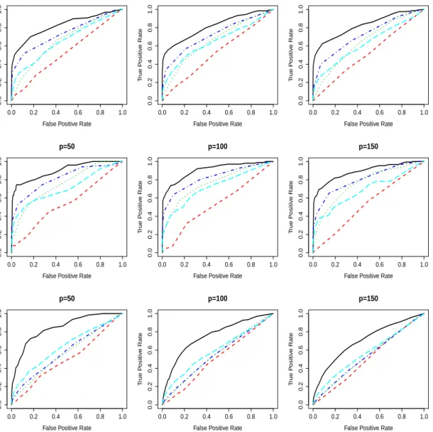
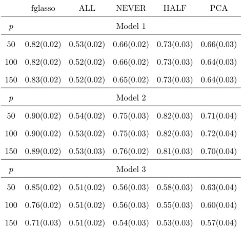
We considered different settings withp= 50,100, 150, and ran each simulation 100 times. Figure2plots the median best ROC curves for each of the five comparison methods, respec-tively for Models 1–3. The fglasso (black curve) clearly had the best overall performance in recovering support of the functional network. Table 1 provides the area under the ROC curves (average over the 100 simulation runs) along with standard errors. Larger numbers indicate superior estimates of the true network structure. Again we see that the fglasso provided highly significant improvements in accuracy for graph recovery over the competing methods in all the settings we considered. Among the four competing approaches, HALF performed the best for Models 1 and 2, and PCA slightly outperformed others for Model 3.
0.0 0.2 0.4 0.6 0.8 1.0 0.0 0.2 0.4 0.6 0.8 1.0
False Positive Rate
T rue P ositiv e Rate p=50 0.0 0.2 0.4 0.6 0.8 1.0 0.0 0.2 0.4 0.6 0.8 1.0
False Positive Rate
T rue P ositiv e Rate p=100 0.0 0.2 0.4 0.6 0.8 1.0 0.0 0.2 0.4 0.6 0.8 1.0
False Positive Rate
T rue P ositiv e Rate p=150 0.0 0.2 0.4 0.6 0.8 1.0 0.0 0.2 0.4 0.6 0.8 1.0
False Positive Rate
T rue P ositiv e Rate p=50 0.0 0.2 0.4 0.6 0.8 1.0 0.0 0.2 0.4 0.6 0.8 1.0
False Positive Rate
T rue P ositiv e Rate p=100 0.0 0.2 0.4 0.6 0.8 1.0 0.0 0.2 0.4 0.6 0.8 1.0
False Positive Rate
T rue P ositiv e Rate p=150 0.0 0.2 0.4 0.6 0.8 1.0 0.0 0.2 0.4 0.6 0.8 1.0
False Positive Rate
T rue P ositiv e Rate p=50 0.0 0.2 0.4 0.6 0.8 1.0 0.0 0.2 0.4 0.6 0.8 1.0
False Positive Rate
T rue P ositiv e Rate p=100 0.0 0.2 0.4 0.6 0.8 1.0 0.0 0.2 0.4 0.6 0.8 1.0
False Positive Rate
T
rue P
ositiv
e Rate
p=150
Figure 2: Model 1(top row), Model2(middle row) and Model3(bottom row) for p= 50,100
and 150: Comparison of median estimated ROC curves over 100 simulation runs for fglasso
(black solid), ALL (red dashed), NEVER (green dotted), HALF (blue dash dotted), and PCA (cyan long dashed).
5.2
EEG Data
We test the performance of the fglasso on the EEG data set from the alcoholism study discussed in Section 1. The study consists of 122 subjects, 77 in the alcoholic group and
Table 1: The mean area under the ROC curves. Standard errors are shown in parentheses.
fglasso ALL NEVER HALF PCA
p Model 1 50 0.82(0.02) 0.53(0.02) 0.66(0.02) 0.73(0.03) 0.66(0.03) 100 0.82(0.02) 0.52(0.02) 0.66(0.02) 0.73(0.03) 0.64(0.03) 150 0.83(0.02) 0.52(0.02) 0.65(0.02) 0.73(0.03) 0.64(0.03) p Model 2 50 0.90(0.02) 0.54(0.02) 0.75(0.03) 0.82(0.03) 0.71(0.04) 100 0.90(0.02) 0.53(0.02) 0.75(0.03) 0.82(0.03) 0.72(0.04) 150 0.89(0.02) 0.53(0.03) 0.76(0.02) 0.81(0.03) 0.70(0.04) p Model 3 50 0.85(0.02) 0.51(0.02) 0.56(0.03) 0.58(0.03) 0.63(0.04) 100 0.76(0.02) 0.51(0.02) 0.56(0.03) 0.55(0.03) 0.60(0.04) 150 0.71(0.03) 0.51(0.02) 0.54(0.03) 0.53(0.03) 0.57(0.04)
45 in the control group. For each subject, voltage values were measured from 64 electrodes placed on the scalp which were sampled at 256 Hz (3.9-ms epoch) for one second. Each subject completed 120 trials under either a single stimulus or two stimuli. The electrodes were located at standard positions (Standard Electrode Position Nomenclature, American Electroencephalographic Association (1990)). Zhang et al.(1995) discuss the data collection process in detail. Li et al.(2010);Zhou and Li(2014) analyze the data treating each covariate as a 256×64 matrix. We focus on the EEG signals filtered at α frequency bands between 8 and 12.5Hz, the case considered in Knyazev (2007), Hayden et al. (2006) and Zhu et al.
(2016). Using 4 representative electrodes from the frontal and parietal region of the scalp
Hayden et al.(2006) found evidence of regional asymmetric patterns between the two groups.
regions. Many authors used multiple samples per subject in order to obtain a sufficiently large sample, violating the independence assumption inherent in most methods. Following the analysis in Li et al. (2010) we only consider the average of all trials for each subject under the single stimulus condition. Thus we have at mostn = 77 observations and aim to estimate a network involving p= 64 nodes/electrodes.
We first performed a preprocessing step using the eegfilt function (part of the eeglab
toolbox) to performαband filtering on the signals. The fglasso was then fitted to the filtered data. The dimension of the B-spline basis function, L, was selected using the same cross-validation approach as for the simulation study. We setM = 6 for this data since 6 principal components already explained more than 90% of the variation in the signal trajectories. Note that since our goal was to provide interpretable visualizations and investigate differences in brain connectivity between the alcoholic and control groups we computed sparse networks with approximately 5% connected edges. To assess the variability in the fglasso fit we performed a bootstrap procedure by randomly selecting n observations with replacement from the functional data, finding a tuning parameterγn to yield 5% sparsity level, applying
the fglasso approach to the bootstrapped data, and repeating the above process 50 times. The “bootstrapped fglasso” was then constructed from the edges that occurred in at least 50% of the bootstrap replications.
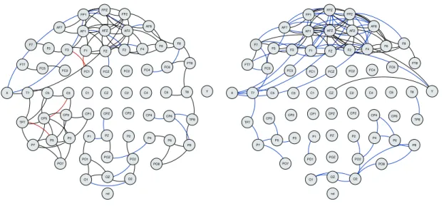
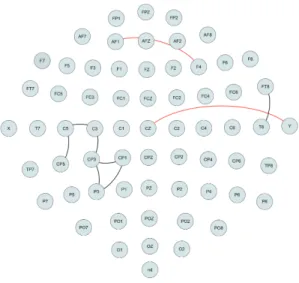
Figure 3 plots the estimated network using the fglasso and the bootstrapped fglasso for both the alcoholic and the control groups. The bootstrapped fglasso estimated a sparser network with sparsity level 4.1% for the alcoholic group and 2.5% for the control group. We observe a few apparent patterns. First, electrodes from the frontal region are densely connected in both groups but the control group has increased connectivity relative to the alcoholic group. Second, the left central and parietal regions of the alcoholic group includes more connected edges. Third, electrodes from other regions of the scalp tend to be only sparsely connected. Finally, the fraction of black to red and blue edges provides a proxy for the level of confidence in any given estimated network. For the alcoholic group this is fairly
FP1 FP2 F7 F8 AF1 AF2 FZ F4 F3 FC6 FC5 FC2 FC1 T8 T7 C3 CZ C4 CP5 CP6 CP1 CP2 P3 PZ P4 P8 P7 PO2 PO1 O2 O1 X AF7 AF8 F5 F6 FT7 FT8 FPZ FC4 FC3 C6 C5 F2 F1 TP8 TP7 AFZ CP3 CP4 P5 P6 C1 C2 PO7 PO8 FCZ POZ OZ P2 P1 CPZ nd Y FP1 FP2 F7 F8 AF1 AF2 FZ F4 F3 FC6 FC5 FC2 FC1 T8 T7 C3 CZ C4 CP5 CP6 CP1 CP2 P3 PZ P4 P8 P7 PO2 PO1 O2 O1 X AF7 AF8 F5 F6 FT7 FT8 FPZ FC4 FC3 C6 C5 F2 F1 TP8 TP7 AFZ CP3 CP4 P5 P6 C1 C2 PO7 PO8 FCZ POZ OZ P2 P1 CPZ nd Y
Figure 3: Left graph plots the estimated network for the alcoholic group and right graph plots the estimated network for the control group. Black lines denote edges identified by both fglasso and bootstrapped fglasso, blue lines denote edges identified by fglasso but not selected by the bootstrapped fglasso and red lines denote edges identified by the bootstrapped fglasso but missed by the fglasso.
high, suggesting an accurately estimated network. However, the ratio is somewhat lower for the control group, suggesting a less accurate estimate. This is not surprising given the challenging data set withp= 64 nodes, corresponding to estimating graphs for 64×6 = 384 variables based on only 45 observations.
To identify edges that were clearly different between the two groups we selected edges that occurred at least 50% more often in the bootstrap replications for one group relative to the other group. Figure 4 plots the edges only identified by either the alcoholic group or the control group. We observe that some edges in the left central and parietal regions were identified by the alcoholic group but missed by the control group, while one edge in the frontal region was identified by the control group but missed by the alcoholic group. Both findings provide confirmation for our informal observations from Figure 3.
Figure 4: Black lines denote edges identified only by the alcoholic group and red lines denote edges identified only by the control group.
6
Discussion
We conclude the paper by discussing three extensions. Here we have assumed that the tra-jectories of the functional variables are fully observed, although our results could be extended to the setting of densely observed curves under extra regularity and smoothness conditions. Hence, the first possible extension involves constructing a graphical model for sparse, irreg-ular and noisy functional data, a common situation in functional data analysis (FDA). This extension could be achieved by performing FPCA on sparsely sampled functional data using either a mixed effects model (James et al., 2000) or a local smoother method (Yao et al.,
2005), and then implementing the fglasso on the conditional expectations of the principal component scores.
Second, one referee was concerned that, since the inverse of the covariance operator of (g1, . . . , gp) is unbounded (Bosq, 2000), then the minimum eigenvalue of the covariance
matrix Σ∗M goes to zero as M → ∞. He/she suggested that the true edge set E could instead be recovered based on the bounded inverse correlation operator, i.e. using the block sparsity pattern in Q∗M, the inverse correlation matrix of aM
using an alternative criterion by replacing the sample covariance matrix, SM, in (9) with the
sample correlation matrix,RM. Specifically, we propose to solve the following optimization
problem
b
QM = argmax
QM
(
log det(QM)−trace(RMQM)−γn
X
j6=l
kQMjlkF
)
, (24)
where the optimization is restricted to be over symmetric positive definite matrices in
RM p×M p such that the diagonal elements of (QM)−1 are one andγn is a non-negative tuning
parameter. We could then use the identified block sparsity structure in QbM to estimate
E. We discuss the connection between our fglasso approach and (24) in Section D.2 of the Supplementary Material and develop an algorithm to solve (24) in Section D.3. Theoreti-cally, however, derivations on the entrywise concentration inequalities for RM are needed, posing additional challenges. It is worth noting that in FDA one usually selects only the first few principal components, so this issue does not pose any practical concern for the fglasso approach.
Third, the main theoretical limitation in this paper is to treat the dimension of the functional variables as approaching infinity rather than truly infinite dimensional functional objects (Mn → ∞ rather than Mn = ∞). It is challenging, under the current framework,
to relax the assumption Mn < ∞ to the fully functional situation with Mn = ∞, since we
would need to write Conditions 3-4 and the relevant proofs in terms of abstract functional analysis language in Hilbert space rather than the current compact matrix forms. We next present another way to understand the conditional dependence structure when Mn < ∞.
From Peng et al. (2009),aijk can be expressed as
aijk= p X l6=j Mn X m=1 βjlkmailm+ijk, i= 1, . . . , j ∈V, k = 1, . . . , Mn, (25)
such that {ijk, k = 1, . . . , Mn} is uncorrelated with {ailm, l ∈ V, l 6= j, m = 1, . . . , Mn} if
and only if βjl=−(Θ∗Mn jj ) −1 Θ∗Mn jl ,(j, l)∈V 2 , l 6=j, (26)
with its (k, m)-th entry given by βjlkm. In other words, both {βjl,(j, l) ∈ V2, j 6= l} and
{Θ∗Mn
jl ,(j, l) ∈ V
2, j 6= l} can be used to identify the true edge set. When M
n = ∞,
although (26) cannot be written in the compact matrix form, the analogy to (25) still holds and {βjlkm, k, m = 1, . . . ,∞} reflects the network structure between nodes j and l. The
expression (25) withMn=∞provides an alternative approach for estimating the FGM, but
would require new algorithms and theoretical guarantees.
Another potential approach to tackle the finite dimensional limitation is to find a large enough value of Mn0 <∞ such that
max (j,l)∈V2,j6=lkC M0 n jl (s, t)−Cjl(s, t)k∗ ≤O(n −ω ), (27)
where k · k∗ denotes some functional norm and ω is some positive value. Intuitively, if
max(j,l)∈V2,j6=lkCM 0 n jl (s, t)−Cjl(s, t)k∗ is small enough, CM 0 n
jl (s, t) provides a good
approxi-mation to Cjl(s, t), hence C Mn0
jl (s, t) can still be used to identify the graph structure. This
formulation then reduces to the model considered in our paper, which assumes large but finite dimensional functional data and our theoretical results become applicable in the more general setting. However, it appears challenging to prove (27) with suitable choices of Mn0
and ω.
These are all fruitful topics for future research but are beyond the scope of this paper.
Acknowledgements.
We are grateful to the Editor, the Associate Editor and three referees for their useful com-ments and suggestions.
A
Appendix
AppendixA.1contains a counterexample where the grid method described in Section 1fails. Further remarks on some regularity conditions are provided in Appendix A.2.
A.1
Counterexample
We create a counterexample, in which the grid method is not able to identify the true conditional dependence structure while our approach can. Take M = 1, p = 3, T = [0,1] and let gj(t) = ajφj(t), j = 1,2,3, where the aj’s are standard normal, a1, a2 are correlated
conditional on a3, φ1(t) = f1(t)I{0≤t≤1/2} and φ2(t) = f2(t)I{1/2<t≤1} with
R1/2 0 f1(t) 2dt = R1 1/2f2(t) 2dt = 1. Then Cov g 1(s), g2(t)|g3(u), u ∈ T = Cov(a1, a2|g3(u), u ∈ T)φ1(s)φ2(t),
which equals zero for all s=t, (s, t)∈ T2, but is nonzero for some s6=t.
A.2
Further Remarks on Some Regualrity Conditions
Remark on Conditions 3–4. We provide an example satisfying Conditions 3 and 4. For convenience, denote aij = (xTij,yTij)T, i = 1, . . . , n, j = 1, . . . , p, where xij = (aij1, . . . , aijM)T
and yij = (aij(M+1), . . . , aijMn)
T. Define
e
Σ ∈ RpMn×pMn to be the covariance matrix of
(xT11, . . . ,xT1p,yT11, . . . ,y1Tp)T. Then we can find a permutation matrixPπ satisfyingP−π1 =PTπ
such thatPπΣPTπ =Σe andΩe =PπΩPTπ,which indicates thatΩe is a permutation ofΩ. Let
e Σ = e Σ11 Σe12 e Σ21 Σe22 and Ωe = e Ω11 Ωe12 e Ω21 Ωe22
, where Σe11, Ωe11 are pM ×pM submatrices
and Σe22, Ωe22 are p(Mn−M)×p(Mn−M) submatrices. If we consider (x11T , . . . ,xT1p)T to
be independent of (yT11, . . . ,y1Tp)T, then Ωe
(k)
12 = 0 for M ≤ k < Mn, i.e. Ω
(k)
jl,2 = 0, for M ≤
k < Mn, which satisfies Condition 3. On the other hand, min(j,l)∈EkΩjlkF corresponds to
the minimal signal strength. In our example, kΩjlk2F =kΩ
(M) jl,1k 2 F+kΩ (M) jl,4k 2 F, so Condition 4
presents a sufficient condition of minimal signal strength.
Remark on Condition 5. It is worth noting that Γ∗ is the Hessian of −log det(Θ) evaluated at Θ = Θ∗. Hence the entry Γ∗(j,j(k,k0)(0l,l)(m,m0) 0) equals
∂(−log det(Θ))
∂Θjj0kk0∂Θll0mm0 evaluated at
Θ=Θ∗, where Θjj0kk0 is the (k, k0)th entry of the M×M submatrixΘjj0, 1≤j, j0, l, l0 ≤p,
1 ≤ k, k0, m, m0 ≤ M. Since a is multivariate Gaussian, some standard calculations show that Γ∗(j,j(k,k0)(0)(l,lm,m0) 0) = Cov (ajkaj0k0, almal0m0). The Hessian of the negative log-determinant for
the scalar data was studied inRavikumar et al.(2011). We extend their work by viewingΓ∗, the Fisher information of the model, as an edge-basedM2-block covariance matrix instead of the node-based covariance matrixΣ∗. For each (j, j0)∈V2, denote bybjj0 =aj⊗aj0 ∈RM
2
the edge-based vector, where aj, aj0 are the node-based vectors. Then we have Γ∗(j,j0)(l,l0) = E(bjj0bT
ll0), which indicates that Condition5is the population version of the
irrepresentable-type condition. Define the edge-based vector withinS bybS ={bjj0,(j, j0)∈S}. Then (21)
is equivalent to||E(bScbTS)E(bSbTS)−1||(M
2)
∞ ≤1−η,which bounds the effects of non-edges in
Sc on the edges inS, and restricts b
jj0’s outside the true edge set S to be weakly correlated
with those within S.
References
Bosq, D. (2000). Linear Processes in Function Spaces, Springer, New York.
Boyd, S., Parikh, N., Chu, E., Peleato, B. and Eckstein, J. (2010). Distributed optimization and statistical learning via the alternating direction method of multipliers,Foundations and Trends in Machine Learning3(1): 1–122.
Cai, T., Liu, W. and Luo, X. (2011). A constrained l1 minimization approach to sparse precision
matrix estimation,Journal of the American Statistical Association 106.
Candes, E. and Tao, T. (2007). The dantzig selection: Statistical estimation whenpis much larger thann,The Annals of Statistics35: 2313–2351.
Danaher, P., Wang, P. and Witten, D. (2014). The joint graphical lasso for inverse covariance estimation across multiple classes, Journal of the Royal Statistical Society: Series B 76: 373– 397.
Friedman, J., Hastie, T. and Tibshirani, R. (2007). Sparse inverse covariance estimation with the graphical lasso,Biostatistics 2: 432–441.
Hayden, E., Wiegand, R., Meyer, E., Bauer, L., O’s Connor, S., J.I., N., D.B., C., B., P. and H., B. (2006). Patterns of regional brain activity in alcohol-dependent subjects, Alcoholism: Clinical and Experimental Research30: 1986–1991.
Hsing, T. and Eubank, R. (2015). Theoretical Foundations of Functional Data Analysis, with an Introduction to Linear Operators, John Wiley & Sons, Ltd.
Ingber, L. (1997). Statistical mechanics of neocortical interactions: Canonical momenta indicators of electroencephalography,Physical Review E55: 4578–4593.
James, G., Hastie, T. and Sugar, C. (2000). Principal component models for sparse functional data,
Biometrika87: 587–602.
Knyazev, G. (2007). Motivation, emotion, and their inhibitory control mirrored in brain osclilla-tions,Neuroscience Biobehavioral Reviews 131: 377–395.
Kolar, M. and Xing, E. (2011). On time varying undirected graphs,Proceedings of Machine Learning Research15: 407–415.
Lam, C. and Fan, J. (2009). Sparsistency and rates of convergence in large covariance matrix estimation,The Annals of Statistics37: 4254–4278.
Li, B., Kim, M. and Altman, N. (2010). On dimension folding of matrix-or array-valued statistical objects,The Annals of Statistics38: 1094–1121.
Mazumder, R. and Hastie, T. (2012a). The graphical lasso: New insights and alternatives,Electronic Journal of Statistics6: 2125–2149.
Mazumder, R. and Hastie, T. (2012b). Exact covariance thresholding into connected components for large-scale graphical lasso,Journal of Machine Learning Research13: 781–794.
Meinshausen, N. and Buhlmann, P. (2006). High dimensional graphs and variable selection with lasso,The Annals of Statistics 34: 1436–1462.
Meinshausen, N. and Buhlmann, P. (2010). Stability selection, Journal of the Royal Statistical Society, Series B72: 417–473.
Peng, J., Wang, P., Zhou, N. and Zhu, J. (2009). Partial correlation estimation by joint sparse regression models,Journal of the American Statistical Association104: 735–746.
Qiu, H., Han, F., Liu, H. and Caffo, B. (2016). Joint estimation of multiple graphical models from high dimensional dependent data,Journal of the Royal Statistical Society: Series B78: 487–504. Ramsay, J. O. and Silverman, B. W. (2005). Functional Data Analysis, 2 edn, Springer.
Ravikumar, P., Wainwright, M., Raskutti, G. and Yu, B. (2011). High-dimensional covariance esti-mation by minimizingl1-penalized log-determinant deivergence, Electronic Journal of Statistics
5: 935–980.
Rice, J. and Silverman, B. (1991). Estimating the mean and covariance structure nonparametrically when the data are curves,Journal of the Royal Statistical Society, Series B 53: 233–243. Storey, J. D., Xiao, W., Leek, T. J., Tompkins, R. G. and Davis, R. W. (2005). Significance
analysis of time course microarray experiments,Proceedings of the National Academy of Sciences
102: 12837–12842.
Sun, T. and Zhang, C. (2013). Sparse matrix inversion with scaled lasso, Journal of Machine Learning Research14: 3385–3418.
Tibshirani, R. (1996). Regression shrinkage and selection via the lasso, Journal of the Royal Statistical Society, Series B58: 267–288.
Tibshirani, R., Saunders, M., Rosset, S., Zhu, J. and Knight, K. (2005). Sparsity and smoothness via the fused lasso,Journal of the Royal Statistical Society, Series B 67: 91–108.
Tseng, P. (2001). Convergence of a block coordinate descent method for nondifferentiable mini-mization,Journal of Optimization Theory and Applications109: 475–494.
Witten, D., Friedman, J. and Simon, N. (2011). New insights and faster computations for the graphical lasso,Journal of Computational and Graphical Statistics 20: 892–900.
Yao, F., Muller, H. and Wang, J. L. (2005). Functional data analysis for sparse longitudinal data,
Journal of the American Statistical Association100: 577–590.
Yuan, M. and Lin, Y. (2006). Model selection and estimation in regression with grouped variables,
Journal of the Royal Statistical Society: Series B68: 49–67.
Yuan, M. and Lin, Y. (2007). Model selection and estimation in the gaussian graphical model,
Zhang, X., Begleiter, B., Porjesz, B., Wang, W. and Litke, A. (1995). Event related potentials during object recognition tasks,Brain Research Bulletin38: 531–538.
Zhou, H. and Li, L. (2014). Regularized matrix regression,Journal of the Royal Statistical Society: Series B76: 463–483.
Zhou, S., Lafferty, J. and Wasserman, L. (2010). Time varying undirected graphs,Machine Learning Journal80: 295–319.
Zhu, H., Strawn, N. and Dunson, D. (2016). Bayesian graphical models for multivariate functional data,Journal of Machine Learning Research17: 1–27.
Zhu, Y., Shen, X. and Pan, W. (2014). Structural pursuit over multiple undirected graphs,Journal of the American Statistical Association109: 1683–1696.
Supplementary Material to “Functional Graphical Models”
Xinghao Qiao, Shaojun Guo, and Gareth M. James
This supplementary material contains the details of the algorithms with derivations in Ap-pendixB, technical proofs of Propositions 1–2, Theorems 1–4, Lemmas1-15in AppendixC, and further discussion in Appendix D.
B
Derivations for the Fglasso Algorithm
In Appendix B, we provide some further details about the fglasso algorithm and the joint fglasso algorithm.
B.1
Step 2(b) of Algorithm
1
Note (14) is equivalent to finding wj1,· · · ,wj(p−1) to minimize
trace p−1 X l=1 p−1 X k=1 SjjwTjl(Θ−−j1)lkwjk+ 2 p−1 X k=1 sTjkwjk ! + 2γn p−1 X k=1 kwjkkF. (B.1)
Setting the derivative of (B.1) with respect to wjk to be zero and applying Lemma 4 yields
∂(B.1) ∂wjk = (Θ −1 −j)kkwjkSjj+ (Θ−j−1)TkkwjkSTjj +X l6=k (Θ−−j1)TlkwjlSTjj+ (Θ −1 −j)klwjlSjj + 2sjk+ 2γnνjk = 2 (Θ−−j1)kkwjkSjj+ X l6=k (Θ−−j1)TlkwjlSjj+sjk+γnνjk ! =0, whereνjk = wjk kwjkkF ifwjk 6=0, andνjk ∈R M×M withkν jkkF ≤1 otherwise,k = 1, . . . , p−1.
We define the block “residual” by
rjk =X
l6=k
If wjk = 0, then krjkkF = γnkνjkkF ≤ γn. Otherwise we need to solve for wjk in the following equation (Θ−−j1)kkwjkSjj +rjk+γn wjk kwjkkF =0. (B.3)
We replace (B.3) by (B.4), and standard packages in R/MatLab can be used to solve the following M2 byM2 nonlinear equation
((Θ−−j1)kk⊗Sjj)vec(wjk) + vec(rjk) +γn
vec(wjk)
kwjkkF
= 0. (B.4)
Hence, the block coordinate descent algorithm for solving wj in (14) is summarized in
Al-gorithm 3.
Algorithm 3 Block Coordinate Descent Algorithm for Solving wj
1. Initialize wjb .
2. Repeat until convergence for k = 1, . . . , p−1.
(a) Compute brjk via (B.2).
(b) Set wbjk =0 if krjkkF ≤γn; otherwise solve for wbjk via (B.4).
B.2
Steps 2(a) and 2(c) of Algorithm
1
At the jth step, we need to compute Θ−−j1 in (14) given current Σ =Θ −1
. Then step 2(a) follows by the blockwise inversion formula. Next we solve for wj via Algorithm 3, and then update Θ−1 given current wj, Θjj, and Θ−−j1, by applying the blockwise inversion formula again. Rearranging the row and column blocks such that the (j, j)-th block is the last one, we
obtain the permuted version ofΘ−1 by
Θ−−j1+UjVjUTj −UjVj −VjUTj Vj ,whereUj =Θ−−j1wj
and Vj = (Θjj−wjTUj)−1 =Sjj. Step 2(c) follows as a consequence.
B.3
Joint Fglasso Algorithm
We put superscript (q) on the terms used in Section 3.1 to denote the corresponding ones for the q-th class, 1 ≤q ≤Q. Then, for a fixed value of Θ(−jq), some calculations show that
(11) with the addition of the penalty (12) is minimized by setting
b
Θjj(q) = (Sjj(q))−1+ (wbj(q))T(Θ(−jq))−1wb(jq), (B.5)
where wbj(1), . . . ,wbj(Q) are obtained by minimizing
Q X q=1 traceS(jjq)(wj(q))T(Θ(−jq))−1w(jq)+ 2(sj(q))Twj(q) (B.6) +2γ1n p−1 X l=1 Q X q=1 kwjl(q)kF + 2γ2n p−1 X l=1 v u u t Q X q=1 ||w(jlq)||2 F,
and w(jlq) represents the lth M ×M block of wj(q). Analogously to the fglasso algorithm, we summarize the joint fglasso algorithm, which is developed to solve the optimization problem (11) in Algorithm 4.
Algorithm 4 Joint Functional Graphical Lasso Algorithm
1. Initialize Θb
(q)
=Iand Σb
(q)
=I, q= 1, . . . , Q.
2. Repeat until convergence for j = 1, . . . , p, q= 1, . . . , Q.
(a) Compute (Θb (q) −j)−1 ←Σb (q) −j −σb (q) j (Σb (q) jj ) −1( b σ(jq))T.
(b) Solve for wb(jq) in (B.6) using Algorithm 5. (c) Reconstruct Σb (q) us