Microstructure noise, realized volatility,
and optimal sampling
∗
Federico M. Bandi
†and Je
ff
rey R. Russell
‡December 23, 2003
Abstract
Recorded prices are known to diverge from their “efficient” values due to the presence of market microstructure contaminations. The microstructure noise creates a dichotomy in the model-free estimation of integrated volatility. While it is theoretically necessary to sum squared returns that are computed over very small intervals to better indentify the underlying quadratic variation over a period, the summing of numerous contaminated return data entails substantial accumulation of noise.
Using asymptotic arguments as in the extant theoretical literature on the subject, we argue that the realized volatility estimator diverges to infinity almost surely when noise plays a role. While realized volatility cannot be a consistent estimate of the quadratic variation of the log price process, we show that a standardized version of the realized volatility estimator can be employed to uncover the second moment of the (unobserved) noise process. More generally, we show that straightforward sample moments of the noisy return data provide consistent estimates of the moments of the noise process.
Finally, we quantify thefinite sample bias/variance trade-offthat is induced by the accumu-lation of noisy observations and provide clear and easily implementable directions for optimally sampling contaminated high frequency return data for the purpose of volatility estimation.
∗We thank Tim Conley and the participants at the CIRANO conference “Realized Volatility,” Montreal, November 7-8, 2003, for helpful discussions. We are especially indebted to Neil Shephard for his valuable comments.
†Graduate School of Business, University of Chicago, 1101 East 58 street, Chicago, IL 60637. ‡Graduate School of Business, University of Chicago, 1101 East 58 street, Chicago, IL 60637.
1
Introduction
A substantial amount of recent work has been devoted to the model-free measurement of volatility
in the presence of high frequency return series (see the review paper by Andersen et al. (2002) and
the references therein). The main idea is to aggregate intra-daily squared returns to approximate
the daily quadratic variation of the semimartingale that drives the underlying log price process. The
consistency result justifying this procedure is the convergence in probability of the sum of squared
returns to the quadratic variation of the log price process as returns are computed over intervals
that are increasingly small asymptotically. While this result is a cornerstone in semimartingale
process theory (see Chung and Williams (Theorem 4.1, page 76, 1990), for instance), the availability
of high frequency return data has made it possible to develop a nonparametric theory of inference
for volatility estimation that heavily relies on its implications (see Andersen et al. (2003a) and
Barndorff-Nielsen and Shephard (2002), BN-S hereafter).
The empirical validity of the procedure hinges on the observability of the true price process.
Nonetheless, it is well-accepted that the true price process and, as a consequence, the return data
are contaminated by market microstructure effects, such as discrete clustering and bid-ask spreads, among others. In other words, asset prices diverge from their “efficient values” due to a variety of market frictions. BN-S (2002) write “...The implication of this is that it is dangerous to make
inference based on extremely large values ofM[whereMis the number of observations] for the effect of model misspecification can swamp the effects we are trying to measure. Instead it seems sensible to use moderate values of M and properly account for the fact that the realized variance error is
not negligible...” In the BN-S’s framework an asymptotic increase in the number of observationsM
translates intofiner andfiner sampling over time for afixed time period of interest. Andersen et al.
(2001) write “... as such it is not feasible to push the continuous record asymptotics ... beyond this
level. ...Such market microstructure features ... can seriously distort the distributional properties
of high frequency intra-day returns.” In their review paper Andersen et al. (2002) write “...it is
undesirable, and due to the presence of market microstructure frictions indeed practically infeasible,
to sample returns infinitely often over infinitesimally short time intervals. Model specific calculations
and simulations by [many authors1] illustrate the effects offiniteM [number of observations, that is] andh[time span] for a variety of settings. The discrepancies in the underlying model formulation
and character of the assumed frictions render a general assessment of the results difficult. Moreover, the size of the measurement errors are often computed unconditionally rather than conditional on
the realized volatility statistic. Nonetheless, it is evident that the measurement errors typically are
non-trivial.”
Usinginfillasymptotic arguments (i.e., increasingly frequent observations over afixed time span) as in the extant theoretical literature on the subject (c.f., Andersen et al. (2003a) and BN-S (2002))
and a realistic price formation mechanism that accounts for microstructure effects (see Madhavan (2000)), we show that the quadratic variation estimates are swamped by noise as the number of
squared return data increases asymptotically. The theoretical manifestation of this effect is a realized volatility estimator that fails to converge to the underlying quadratic variation of the log price process
but, instead, diverges to infinity almost surely over any period of time, however small. This result
provides a theoretical justification for the diverging behavior at high frequencies of the realized
volatility estimates of liquid stocks as reported by Andersen et al. (2000).
Interestingly, despite the fact that realized volatility is not consistent for the conventional object
of interest (quadratic variation, that is), a standardized version of the realized volatility estimator
can be employed to identify a specific feature of the noise distribution (rather than a feature of the
true return process, as generally believed), namely the variance of the (unobservable) noise process.
More generally, we show that straightforward sample moments of the contaminated return data can
be employed to identify the moments of the underlying noise process.
As stressed earlier, we are not the first ones to point out the potential impact of market
mi-crostructure frictions on volatility estimates obtained through aggregation of high frequency squared
return data. Nonetheless, while previous discussions of the potential role played by microstructure
contaminations are based on informal arguments, rigorous limiting results provide justification for
aggregation as a means to uncover, in the limit, the true quadratic variation of the underlying log
price process. To this extent, the present paper fills a gap in the existing literature by illustrating
the theoretical implications of the presence of microstructure noise on the asymptotic results that
are generally invoked to justify quadratic volatility estimation through aggregation of high frequency
squared return data.
An important remark is worth making at this point. The use of increasingly frequent observations
as a requirement for consistency in nonparametric (point-wise) continuous-time model estimation
results needs to be interpreted as an asymptotic approximation. Just like the more standard “large
n” requirement is meant to signify sufficient accumulation of information, the infill requirement signifies sufficient information in the vicinity of the level at which point-wise estimation is performed. In practise, while the infill approximation permits identification under mild assumptions on the
properties of the process of interest (thereby not requiring often difficult stationary density-based identification procedures), its empirical validity is known not to hinge on the availability of high
frequency observations being that daily sampling is generally sufficient for the approximation to apply (the interested reader is referred to the review paper by Bandi and Phillips (2002) and the
references therein for discussions). To this extent, the issue of quadratic variation estimation is
fundamentally different from the point-wise identification of continuous-time models in that the very nature of the problem makes the theoretical need for high-frequency return data a stringent
empirical requirement in the former case, thereby justifying a closer investigation into more realistic
limiting results. This is what the present work hopes to achieve in one of its contributions.
Having made these observations, natural remaining issues are how to formalize thefinite sample
loss that is induced by a realistic noise component in volatility estimation, and how to employ this
information to fully exploit the identification potential of the empirically important notion of realized
volatility as introduced by Andersen et al. (2003a) and BN-S (2002).
In keeping with the model-free spirit of the realized volatility literature, we tackle this issue by
deriving the conditional (on the underlying volatility path) mean-squared error (MSE, henceforth)
of the contaminated volatility estimator. Specifically, we show that the presence of microstructure
noise induces a finite sample bias/variance trade off. The idea is simple. When the true price process is observable, as typically assumed in conventional theoretical models, the larger is the
sampling frequency over afixed period of time, the more precise is the estimation of the integrated
volatility (or quadratic variation) of the log price process. When the true price process is not
observable, as typically the case in practise, frequency increases provide information about the
underlying integrated volatility but, necessarily, entail accumulations of noise that affect both the bias and the variance of the estimator. The optimal sampling frequency should be chosen to balance
these two contrasting effects. We formalize these ideas by deriving the expression that ties the properties of theconditionalMSE of the contaminated quadratic variation estimator to the features
of the microstructure noise distribution. The idea is therefore similar in spirit to Bai et al. (2000)
Finally, we provide a methodology to optimally choose the sampling frequency as the minimum
of the conditional expected squared distance between the estimator (i.e., realized volatility) and
its theoretical counterpart (i.e., quadratic variation), as summarized by the conditional MSE. The
method relies on the computation of sample moments of contaminated high frequency return data
as well as on the minimization of a simple nonlinear function. As such, it is straightforward to
implement. We also provide a rule-of-thumb for selecting the optimal frequency without having to
implement an otherwise simple minimization routine. Since the rule-of-thumb takes the familiar
form of a signal-to-noise ratio (thereby highlighting the main determinants of the optimal sampling
frequency), we expect it to be useful in applied work on the subject.
The paper proceeds as follows. In Section 2 we lay out the model. Section 3 is about the
limiting properties of the realized volatility estimator when microstructure noise affects fair prices in a realistic manner. In Section 4 we present an expansion of the conditional MSE of the quadratic
variation estimator when noise plays a role and discuss optimal sampling through minimization of
the conditional MSE. In Section 5 we illustrate the implications of ourfindings when estimating the
quadratic variation of the log price process as well as the second moment of the (unobservable) noise
process in the presence of quote-to-quote IBM price changes. The analysis is Section 5 is conducted
through empirical work and simulations. Section 6 concludes. Proofs and technical details are in
Appendix A. Appendix B lays out the notation.
2
The model
The model we study is coherent with previous theoretical approaches to model-free volatility
esti-mation. Specifically, we employ the same underlying set-up as in BN-S (2002, 2004) but explicitly
introduce realistic microstructure effects. The notation is also consistent with BN-S (2002, 2004). We consider a fixed time period h (a trading day, for instance) and write the observed price
process as
e
pih=pihηih i= 1,2, ..., n, (1)
wherepihis the true price andηih denotes microstructure noise. A simple log transformation gives
ln (peih)−ln ¡ e p(i−1)h ¢ | {z } e ri = ln(pih)−ln(p(i−1)h) | {z } ri +ηih−η(i−1)h | {z } εi i= 1,2, ..., n, (2) whereη= ln(η).
Assumption 1. (The price process.)
(1) The log price process ln(pih)is a continuous local martingale. Specifically,
ln(pih) =Mih, (3)
where Mih=R0ihσsdWsand {Wt:t≥0}is a standard Brownian motion.
(2) The spot volatility process σt is c`adl`ag and bounded away from zero.
(3) σt is independent of Wt ∀t.
(4) The integrated variance process Vt=R0tσ2sds <∞ ∀t <∞.
We divide the period hinto M subperiods and define the observed high frequency returns as
e rj,i= ln¡pe(i−1)h+jδ ¢ −ln¡ep(i−1)h+(j−1)δ ¢ j= 1,2, ..., M, (4)
whereδ=h/M. Hence,erj,iis thej-th intra-day return for dayi. Naturally then,
e
rj,i=rj,i+εj,i, (5)
whererj,iandεj,i(=η(i−1)h+jδ−η(i−1)h+(j−1)δ) have straightforward interpretations given Eq. (2) above.
Assumption 2. (The microstructure noise.)
(1) The random shocks ηj are iid mean zero with a bounded eight moment.
(2) The true return process rj,i is independent of ηj,i∀i, j.
Lemma 1 below illustrates the moments of the noises-in-returnsε0s as a function of the moments
Lemma 1. Under the specification in Eq. (2) the following relations hold: (1) E(ε2) = 2E(η2), (2) E(ε4) = 2E(η4) + 6¡E(η2)¢2, (3) E(ε2ε2 −1) = 3 ¡ E(η2)¢2+E(η4).
Proof. See Appendix A.
Lemma 2 relates the first order cross-moment of the squared noises-in-returns to the fourth
moment of the noise-in-return.
Lemma 2. Under the specification in Eq. (2) the following relation holds:
E(ε2ε2−1) =1 2E(ε
4). (6)
Proof. Immediate given results (2) and (3) in Lemma 1.
Some observations on the set-up are needed. The true return process r is modelled as a
lo-cal martingale with bounded variance E(r2
j,i) equal to E ³R(i−1)h+jδ (i−1)h+(j−1)δσ 2 sds ´
over any period δ
(c.f., Assumption 1(1) and 1(4)). The spot volatilityσ is allowed to display jumps, diurnal effects, long-memory features,2 and nonstationarities (c.f., Assumption 1(2)). Consistently with existing
theoretical treatments (see BN-S (2002, 2004), for instance), we rule out leverage effects (c.f., As-sumption 1(3)). Nonetheless, while the extant literature has pointed out that the presence of leverage
generally induces second-order effects (Andersen et al. (2003b), BN-S (2003), and Meddahi (2002), among others), in the sequel (see Section 3 and Appendix A below) we show that our limiting results
(as represented by Theorem 1 and 2) are robust to the existence of leverage.
The econometrician does not observe r, the true return series, but a contaminated return series e
rwhich is given by r plus a random shockε that is independent ofr (c.f., Assumption 2(2)). We
interpret theε0s as being microstructure contaminations in returns. In virtue of the specification in
Eq. (2) above and Assumption 2(1), the shocksε0s are identically distributed with a bounded eight
moment. Nonetheless, they are not uncorrelated since theirfirst-order autocovariance is negative and
2Long-memory is known to be an important feature of volatility series. The interested reader is referred to Bandi
equal to−E(η2) =−σ2
η, i.e., the variance of the underlying shocksη 0
s taken with a negative sign.
The negativefirst-order autocorrelation of the microstructure contaminations in returns determines
an analogousfirst-order autocorrelation in the contaminated return series. This feature of the noise
specification captures a well-known empirical fact (see Niederhoffer and Osborne (1966), Cohen et al. (1979), and Roll (1984) for some earlyfindings). In Section 5 we confirm this fact for IBM. Using
mid-point bid ask quotes, in a companion paper wefind strong negativefirst-order autocorrelations (and
higher-order autocorrelations that are economically negligible and often statistically insignificant)
for the majority of the S&P 100 stocks (Bandi and Russell (2003b)).
While being supported by a vast empirical evidence, the structural model implied by Eq. (1)
appears to be a natural set-up to analyze the impact of microstructure contaminations on the realized
volatility estimates. In effect, well-known canonical microstructure models with trading frictions and private information can easily be cast into our framework. One early example is Roll’s implicit
bid-ask model (Roll (1984)). The interested reader is referred to Campbell et al. (1996) and the review
paper by Madhavan (2000) for a complete discussion of Roll’s price formation mechanism and recent
advances. It is noted that A¨ıt-Sahalia and Mykland (2003) adopt a similar set-up in their analysis
of the impact of microstructure noise on the parametric (i.e., maximum likelihood) estimates of the
second infinitesimal moment of scalar diffusion models.
There is a subtle reason, which has to do with the orders of magnitude of the quantities involved,
why we expect the model in Eq. (2) to capture the main effects in high-frequency data. The idea goes as follows. Different trading institutions and different price measurements potentially have different microstructure characteristics which, in turn, determine and characterize η. Generally speaking,
high-frequency financial data provide both bid and ask prices as well as transaction prices. It is
common practice to use the mid-point of the prevailing bid and ask prices as a (noisy) measure
of the true price. In fact, actual transaction prices suffer from well-known bid ask bounce effects and are thought to be more noisy than the midpoint of the quote measurements. In agreement
with this observation, the empirical work in this paper focuses on mid-points of bid and ask quotes.
Specifically, our methodology exploits a fundamental difference in the nature of the true returns and the noise associated with its mid-quote observations. The efficient price is considered a continuous process. It is the price that would prevail in the absence of market frictions. Thus, the dynamics of
the efficient price should be driven by a smooth process reflecting the continual updating and learning on the part of the market participants. In effect, it takes time for the market participants to react and
digest new information. Hence, with the exception of important rare public news announcements, the
price will not likely jump from one level to another, but rather smoothly adjust as the market comes
to grips with any new information. The characteristics of the noise are substantially different from the true price characteristics since posed quotes in a market inherently reflect different information than the efficient price. Observed prices are not permitted to vary continuously, but rather fall on a fixed grid of prices or ticks. Changes in the mid-quotes are therefore discrete in nature.
Furthermore, classic microstructure theory suggests that a market maker posting quotes will take
into consideration the nature of the limit order book, current inventory levels, as well as the risks
associated with asymmetric information. Adjustments to these components are necessarily discrete
in nature as new limit orders are submitted or a large market order consumes all of the limit orders
at some given price. The transaction process is also thought to carry information regarding the
likelihood of asymmetric information suggesting that this component may also adjust discretely.
When one accounts for the fact that adjustments to the information used to post the quotes are not
smooth coupled with the fact that observed prices must fall on a grid of tick values, it is natural to
consider the departures of the observed price from the true price as a discontinuous process. Hence,
provided we do not sample at a rate faster than new price information arrives (i.e., between quote
updates), the noise in the observed price process should be roughly i.i.d and therefore consistent
with our assumed structure.
Having made these points, we can easily generalized the noise process to more involved
cor-relation structures without changing the main results in the paper. It will be clear that richer
dependence features in the noise process simply determine a more complicated variance expression
in the asymptotic distribution of the (standardized) realized volatility estimator in Section 3 as well
as a more involved (but estimable) variance term in the conditional MSE expansion in Section 4.
Coherently with Andersen et al. (2003a) and BN-S (2002) we define the realized volatility
estimator for the generic periodias
b Vi= M X j=1 e rj,i2 . (7)
We use Vib to estimate Vi =R(ihi−1)hσ2sds, i.e., the quadratic variation of the log price process over
the same period. In the next section we discuss the asymptotic properties of Vib. As pointed out earlier, in agreement with the existing literature on the subject, our asymptotics are conducted by
increasing the number of observationsM over afixed time spanh.
3
Microstructure noise and the limiting distribution of the
realized volatility estimator
We can rewrite the realized volatility estimator in Eq. (7) as the sum of three components, namely
b Vi= M X j=1 r2j,i | {z } Ai + M X j=1 ε2j,i | {z } Bi + 2 M X j=1 rj,iεj,i | {z } Ci . (8)
If the true price process were observable, only the termAi would drive the limiting properties ofVib
(as in BN-S (2002)). The presence of microstructure noise introduces two additional components,
i.e.,Bi andCi. We will show that it is mainly termBi that makes standard consistency arguments
fail. Intuitively,Bidiverges to infinity almost surely as the number of observations increases
asymp-totically (or, equivalently, as the frequency of observations increases in the limit) since more and
more noise is being accumulated for afixed period of time h.
Theorem 1 below contains a characterization of ourfindings.
Theorem 1. If Assumptions 1 and 2 are satisfied, then
b Vi a.s. → M→∞∞ ∀i. (9) Furthermore, √ M Ã b Vi M −E ¡ ε2¢ ! ⇒ M→∞N ¡ 0,V¡ε2¢+ 2E¡¡ε2−E¡ε2¢¢ ¡ε2−1−E¡ε2¢¢¢¢ ∀i, (10) which implies √ M Ã b Vi M −2E ¡ η2¢ ! ⇒ M→∞N ¡ 0,4E¡η4¢¢ ∀i, (11) or, equivalently, √ M Ã1 2Vbi M −E ¡ η2¢ ! ⇒ M→∞N ¡ 0,E¡η4¢¢ ∀i. (12)
Proof. See Appendix A.
Some remarks are in order.
Remark 1. The asymptotic properties of term Ai are known. Specifically, Ai converges in
probability to the underlying quadratic variation of the log price process over the period, namely
Vi =R(ihi−1)hσ2sds(Chung and Williams (1990), for instance). Its asymptotic distribution is mixed-normal and can be expressed as
r
M
h (Ai−Vi)M⇒→∞MN(0,2Qi), (13)
where Qi =R(ihi−1)hσ4dsis the so-called quartic variation (BN-S (2002)). The interested reader is referred to BN-S (2002) for an introduction to the notion of quartic variation and for a thorough
discussion of the above weak convergence result. In the Appendix we provide a proof of the same
result that employes different techniques borrowed from semimartingale process theory. Specifically, we generalize the BN-S (2002)findings, as represented by Eq. (13) above, to a functional central
limit theorem specification while relaxing the assumption of no leverage effects.
Remark 2. The limiting features of term Bi can be studied by using standard methods for
sta-tionary mixing sequences (see Hamilton (1994), for instance). In effect,
√ M µ Bi M −E ¡ ε2¢ ¶ ⇒ M→∞N ¡ 0,V¡ε2¢+ 2E¡¡ε2−E¡ε2¢¢ ¡ε2−1−E¡ε2¢¢¢¢. (14) As pointed out earlier, the form of the asymptotic variance term depends on the specific correlation
structure of the microstructure noise as defined by Eq. (2) and Assumption 2(1). Naturally, a richer
specification would not affect the empirical significance of the limiting results reported in this section and could be easily accounted for.
It is apparent that boundedness of the fourth moment of the noise process is all that is required
for the above weak convergence result to be true. We impose boundedness of the eight moment (c.f.,
Assumption 2(1)) for the statement in Theorem 2 below to be satisfied. Of course, this property
ought to be true by virtue of the fact that the noise process is bounded in practise.
Remark 3. The asymptotic features of termCirely on embedding arguments for local martingales.
Ci ⇒ M→∞MN ¡ 0,2σ2ηVi ¢ . (15)
Intuitively, the sum that constitutesCidoes not diverge to infinity as the number of observationsM
increases without bound since each noise term is multiplied by increasingly smaller random returns.
Remark 4. Remark 1 through 3 imply that
Ai+Bi+Ci = µ Vi+Op µ 1 √ M ¶¶ +ME¡ε2¢+Op³√M´+Op(1) a.s.→ M→∞∞, (16)
asM → ∞, thereby justifying thefirst statement in Theorem 1. Divergence to infinity is induced by termBi in that the summing of increasingly frequent squared return data causes infinite
accu-mulation of noise.
Remark 5. We can standardize the realized volatility estimates byMand consider the estimation
error decomposition given by
b Vi M −E ¡ ε2¢ = Ai+Bi+Ci M −E ¡ ε2¢ (17) = Rih (i−1)hσ 2 sds M +Op µ 1 M3/2 ¶ + µ Bi M −E ¡ ε2¢ ¶ +Op µ 1 M ¶ . (18)
Thus, the expression
√ M Ã b Vi M −E ¡ ε2¢ ! =√M µ Bi M −E ¡ ε2¢ ¶ +Op µ 1 √ M ¶ (19)
justifies the second statement in Theorem 1. Interestingly, even though one cannot consistently
estimate the underlying quadratic variation using Vbi when noise is present, a standardized version
of the quadratic variation estimator allows us to identify the second moment of the (unobservable)
noise process by exploiting the asymptotic properties of the dominating termBi.
Lemma 3. While one can consistently estimate the second moment of the noise process, i.e.,
E¡ε2¢, using Vbi
M and characterize the finite sample bias of the realized volatility estimator condi-tionally on the volatility path, namely
bias=ME¡ε2¢,
one cannot hope to consistently estimate Vinonparametrically using Vib by controlling for the existing (increasing-in-M)bias term.
Hence, any statement about the informational content of the conventional realized volatility
estimator as a measurement of the quadratic variation of the underlying log price process ought
to be a finite sample statement. Contrary to common intuition, consistency arguments based on
limitingfindings can only be invoked when estimating features of the noise distribution. The second
moment of the noise process is, of course, not an exception. In Theorem 2 below we show that a
simple arithmetic average of fourth powers of the contaminated return series converges to the fourth
moment of the unobserved noise-in-return process. While it is clear that the procedure is general
enough to be applicable to a variety of different moments (including cross-correlations), for brevity we focus on the fourth moment of the noise process in that it will be a necessary input to formulate
an optimal sampling theory forVbi as an estimator of the quadratic variation of the underlying log
price process.
Theorem 2. If Assumptions 1 and 2 are satisfied, then
1 M M X j=1 e rj,i4 →p E¡ε4¢. (20)
Proof. See Appendix A.
We now move from asymptotic arguments to a characterization of thefinite sample bias/variance
trade-off that is induced by noise accumulation. Specifically, we derive the MSE of the realized volatility estimator conditionally on the volatility path. Our strategy will be to learn about the
underlying quadratic variation of the log price process through the minimization of the conditional
Eσ ³ b Vi−Vi ´2 =Eσ M X j=1 e r2j,i− Z ih (i−1)h σ2sds 2 . (21)
In the next section we show that the MSE does not converge to zero as the sampling frequency
increases without bound. Specifically, the minimum MSE is achieved for afinite number of
observa-tionsM∗. Naturally,M∗ depends on the moments of the microstructure noise distribution as well
as on the quarticity of the underlying log price process.
4
The conditional MSE and optimal sampling
The conditional MSE of the integrated volatility estimator can be represented as in Theorem 3
below.
Theorem 3. If Assumptions 1 and 2 are satisfied, then
Eσ Ã b Vi− Z ih (i−1)h σ2 sds !2 = 2 h M (Qi+oa.s.(1)) +Mβ+M 2α+γ, (22)
where the parameters α,β,and γ are defined as follows:
α = ¡E(ε2)¢2, (23) β = E¡ε4¢+ 2E(ε2ε−21)−3¡E(ε2)¢2, (24) and γ= 4E(ε2)V i−2E(ε2ε2−1) + 2 ¡ E(ε2)¢2. (25)
Proof. See Appendix A.
Should the return series not be affected by the microstructure noise, then the conditional MSE of the quadratic variation estimator would decrease to zero in the limit as the number of observations
diverges to infinity. In effect, the MSE would reduce to the conditional variance of the sum of squared returns, i.e., 2Mh (Qi+oa.s.(1)) (see BN-S (2002) and Appendix A for a derivation).
When microstructure noise is present, Eq. (22) clarifies that the conditional MSE does not
sampling frequency increases over time). Summing up contaminated squared returns induces both
an additional variance term and a bias termEσ(Vbi−Vi) that have the potential to affect substantially
the conditional MSE decomposition. The form of the additional variance term is
ME(ε4) + 2(M−1)E(ε2ε2−1) + (2−3M) (E(ε2))2+ 4E(ε2)Vi, (26) where E(ε4), E(ε2ε2−1), and E(ε2) are obvious moments of the noise-in-return distribution (see
Lemma 1 above) while 4E(ε2)Viis an interaction term. The form of the bias isME(ε2). Apparently,
both quantities diverge to infinity linearly withM, thereby inducing quadratic growth to infinity
(withM) of the corresponding MSE. The coefficientsβ andγ depend on the correlation structure of the noise. Their expressions can be readily modified to account for higher order (up toM−1) correlations as follows: β = E¡ε4¢+ 2 s X b=1 E¡ε2ε2−b¢−(2s+ 1)¡E(ε2)¢2, (27) γ = 4E(ε2)Vi−2 s X b=1 bE¡ε2ε2−b¢+s(s+ 1)¡E(ε2)¢2. (28) Thus, the set-up that we propose is general enough to allow for unrestricted distributional
assump-tions on the noise-in-returnsεas well as more involved dependence features.
Our approach relates to previous work on volatility estimation. Bai et al. (2002) are thefirst to
suggest an MSE expansion for unconditional volatility estimates in the presence of microstructure
noise. Their framework, though, does not provide implications about how moments at different frequencies relate. A¨ıt-Sahalia and Mykland (2003) and Oomen (2003) study MSE values at diff er-ence frequencies in the preser-ence of noise. While A¨ıt-Sahalia and Mykland (2003) derive closed-form
expressions for the unconditional MSE of the constant variance estimator of a drift-less diffusion when (Gaussian) noise plays a role, Oomen (2003) uses a structural model of price formation to
provide simulated MSE plots for noisy quadratic variation estimates as a function of the sampling
interval in the absence of a closed-form specification for the relation between the relevant MSE and
the sampling frequency. Consistently with Oomen (2003), we focus on the quadratic variation of a
local martingale with time-varying stochastic variance. Coherently with A¨ıt-Sahalia and Mykland
(2003), we provide a closed-form expression for the corresponding MSE expansion as a function of
We now turn to optimal sampling. Using Eq. (22) above, we define the optimal number of
observations (per unit intervalh) as the number M∗ which satisfies the following condition:
½ M∗:= arg min µ 2h M (Qi+oa.s.(1)) +Mβ+M 2α+γ ¶¾ (29) or, equivalently, © M∗:=M: 2M3α+M2β−2h(Qi+oa.s.(1)) = 0ª, (30) where the constant termsα,β,andγwere defined earlier.
Lemma 4. (A useful rule-of-thumb for applications.) For high (optimal) frequencies,
M∗∼ Ã hQi (E(ε2))2 !1/3 , (31)
where Qi is the realized quartic variation and E(ε2)is the second moment of the noises-in-returns.
Proof. Immediate given Eq. (29).
Interestingly, when the quadratic term in Eq. (29) dominates the linear term (for values of M
sufficiently large), the approximation in Eq. (31) provides a very good representation of the optimal number of observationsM. In Section 5 we show that this property holds for a very liquid stock like
IBM. Bandi and Russell (2003b) confirm the validity of this result for a large number of S&P100
stocks.
Lemma 4 is important for two reasons. First, it provides us with a very handy and immediate
rule-of thumb to choose the optimal M without having to go through an otherwise rather simple
minimization routine as in Eq. (29). Second, it clearly illustrates what the main determinants
of the optimal frequency are, namely the underlying quarticity of the log price process and the
(squared) variance of the noise-in-returns. Naturally,M∗ can be regarded as a signal-to-noise ratio:
the stronger the signal is, the higher the optimal frequency should be.
4.1
Estimating the optimal sampling frequency
Eq. (30) can be readily solved numerically in the presence of consistent estimates of the quarticity
BN-S (2002) provide an estimator of the quarticity that is consistent in the absence of
microstruc-ture frictions, i.e., Qbi = M3hPjM=1er4j,i. Inevitably, Qbi loses its consistency features in the presence
of the price formation mechanism implied by Eq. (1). Although Qi cannot be consistently
esti-mated using Qib , the simulations in the next section show that the use of different estimates of it (as provided by values ofQib computed on the basis of frequencies that are widely employed in the existing applied work) does not have any considerable impact on the optimal sampling frequency of
the realized volatility estimator.
While we can provide informative estimates ofQi, the availability of high frequency data, along
with the results reported in Theorems 1 and 2 above, allow us to consistently estimate the remaining
inputs of the minimum problem in Eq. (30), i.e., the second and fourth moment of the microstructure
contaminations. More precisely, since our model implies E(ε2ε2
−1) = 2E ¡
ε4¢ (c.f., Lemma 2), Theorem 1 and 2 provide a simple strategy to identify all of the relevant moments of the noise
distribution by simply averaging powers of the contaminated high frequency return data.
As pointed out earlier, even though noisy return data collected at high frequencies do not permit
us to identify the object of interest, i.e., quadratic variation, using the conventional realized volatility
estimator, they do allow us to estimate features of the microstructure contaminations. We use those
features to learn about quadratic variation through the solution of Eq. (30) above.
Onefinal observation is needed. The conditional MSE in Eq. (22) applies to individual periods
h, thereby requiring repeated applications of the procedure. We can readily obtain an optimal (h
-period) frequency M∗ that is valid for the entire data set by simply working with an integrated
version of the conditional MSE in Eq. (22). In other words, we can minimize the average (overi) of
the individual conditional MSE’s. Apparently, this procedure coincides with solving the program in
Eq. (30) above with n1Pni=1Qi, where ndenotes the number of periodsh, in place ofQi.
In Section 5 we provide an application of our methodology to quote-to-quote IBM return data.
5
The case of IBM
5.1
How big is the
unobserved
noise component of the
observed
IBM
price process?
This section explores the magnitude of the unobserved noise component of the observed IBM price
process. Theorem 1 implies that a rescaled version of the realized volatility estimator converges
provides a good estimate of the variance of the (unobservable) microstructure noise. Ideally, we
would like to sample quote-to-quote, the highest frequency that new price information appears.
Our data consists of quote-to-quote changes in the midpoint of posted bid and ask prices. The
quotes were obtained from the TAQ data set for the month of February 2002. Restricting our
attention to NYSE updates, and after removing any suspicious quotes, we are left with 41,841 quote
price updates over the month. On average a new price quote arrives every 10.6 seconds. The midpoint
of the price quotes are used to construct quote-to-quote returns. The smallest return is−2.9% and the largest is.9167%. Thefirst-order autocorrelation is significantly negative and equal to−0.541. The higher order autocorrelations are generally insignificant. Naturally, the largest autocorrelation
(after the first one) is the second-order autocorrelation whose value is equal to 0.048. While this
estimate is statistically significant, its magnitude is virtually ten times smaller (in absolute value)
than the corresponding value for thefirst-order autocorrelation. Thus, our model captures the main
effects in the data.
The square root of the rescaled realized volatility (computed over a 6.5 hour trading period) from
Theorem 1 and Remark 5 is .0278%. Notice that this estimate is essentially the sample standard
deviation imposing a mean return of zero. If we instead usefixed intervals of 30 seconds, the square
root of the rescaled variance increases to.0599%. To put this in dollar context, consider that the
average price for IBM over the month of February in our sample was around 100 dollars. Also, recall
that the variance of the noise termηin Eq. (2) is one half the variance of the return contamination
ε. Thus, the standard deviation of the log noise obtained from the quote-to-quote price moves is
given byση =.000278/√2 =.000197. Sinceση ∼ση, whereη= exp(η), then the standard deviation of the (average) IBM price over the period is about 2 cents. For added perspective, the average
spread for IBM in our sample is 7.2 cents. Hence, the standard deviation is small relative to the
spread with about a +/−2 standard deviation interval just about equal to the average spread. The estimated magnitude of the noise variance seems very plausible.
In finite samples, it is clearly the magnitude of the noise variance relative to the variance of
the “true” return that is of interest. We therefore calculate the realized volatility for each day in
the sample using 15-minute time intervals. While realized volatility remains upward biased in the
presence of noise even at the 15-minute sampling frequency we still believe this statistic is useful
as a benchmark. Our belief, which is consistent with conjectures that have been put forward in the
in the next subsection. The mean realized volatility over the month of February yields an estimate
of the daily standard deviation of 1.652%. Thus, wefind that the noise variance is.01422% of the
typical (average) realized volatility. Naturally, this is a conservative assessment in that the realized
volatility estimates based on 15-minute time intervals are slightly inflated by residual noise.
5.2
The bias in the realized volatility estimates: simulations based on
IBM
This subsection of the paper simulates data from the model given in Eq. (2) using realistic parameter
values based on IBM. From the simulated data estimates of the realized volatility can be compared
to the value of the true quadratic variation. Consistently with the results in Theorem 1, we show
that the realized volatility does indeed explode as the sampling interval goes to zero. We also
show that the appropriately standardized realized volatility converges to the variance of the noise
process. Finally, for the parameter values used, we show that a relatively small bias is present in the
realized volatility estimates at sampling intervals around 15 minutes. Nonetheless, the bias can be
considerable at higher frequencies. For instance, it can be substantial at the commonly-employed
(in applied work) 5 minute interval.
Simulations require specifying a process for both the spot volatility σas well as the noise term
η.As in BN-S (2003), we adopt a square root specification for the evolution of the spot volatility.
Specifically, the infinitesimal variation of the true price process is given by
dlog(p)t=σtdWt1, (32)
where
dσ2t =κ³−v−σ2t´dt+ωσtdWt2. (33)
Further, assuming that the logged noises η are i.i.d. Gaussian completes the specification of the
observed return series as given in Eq. (2) above.
We now turn to selecting parameters for the dynamics of the price and noise processes. The
parameterκdictates persistence in volatility and is set equal to.01, a value consistent with estimates
obtained from simple one-factor continuous-time models. We normalize the mean volatility to unity
so that−v is one. The parameterω controls the magnitude of the volatility of volatility and is set
a variance equal to (.000197)2 (as in the previous section). This implies that the noises-in-returns
ε0s have a variance equal to.02829% of the average daily variance . This value is equal to.000289
since the average variance is normalized to one.
We focus our simulations around a single realization of the (daily) volatility over a period of
6.5 hours. Specifically, we simulate second-by-second a volatility path given by Eq. (33). The initial
value ofσ2is set to the unconditional mean of one. Holding the volatility pathfixed, we then simulate
second-by-second true returns from Eq. (32) and second-by-second observed returns as in Eq. (2).
The simulations are run 1,000 times.
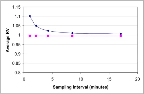
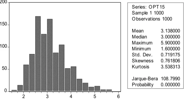
Fig. 1 shows the mean realized volatility across the 1,000 simulations for various sampling
intervals ranging from 1 second to 17 minutes. The horizontal line denotes thefixed (and known)
quadratic variation simulated for the day (i.e., 0.9957). Consistently with the predictions of Theorem
1, the sharp spike at zero shows the realized volatility exploding as the sampling interval goes to zero.
Hence, the standard realized volatility estimator cannot be a consistent estimate of the quadratic
variation of the underlying log price process in the presence of microstructure noise.
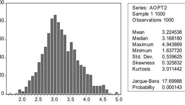
Fig. 2 is the same graph as Fig. 1 plotted on a different scale. This plot shows that, for the parameter values used in the simulation, the bias is small at 15 minutes and, consequently, as the
sampling interval exceeds 15 minutes. At the 17 minute horizon, for instance, the value of the true
quadratic variation is 0.9957 whereas the value of the (average) realized volatility estimate is about
1.006 implying a bias equal to about 1% of the underlying quadratic variation. At the 5-minute
horizon the bias is around 2.5%.
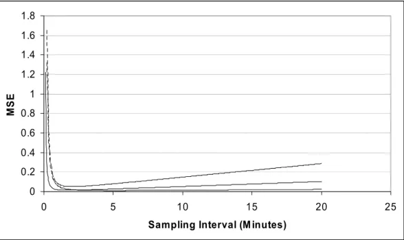
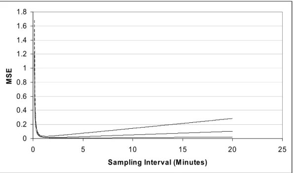
Two observations are in order. First, the only dimension along which Figs. 1 and 2 (which
could be regarded as simulated “volatility signature plots,” using the terminology in Andersen et al.
(2000)) allow us to evaluate the accuracy of the quadratic variation estimates is bias. Naturally, the
optimal sampling frequency should also account for the variance of the sampling error being that
the trade-offbetween bias and variance is apparent (see Fig. 3). The optimal choice of frequency should then balance the low bias at low frequencies with the low dispersion at high frequencies as
discussed in Section 4 above.
Second, the estimated bias depends on a ratio between variance of the noise and quadratic
variation equal to about.0284%. In Fig. 4 we show that the in-sample variability of the estimated
(daily) ratio for IBM is substantial. Specifically, the maximum value of the ratio in our sample is
when the ratio is higher. For clarity, we also perform simulations for a value of the ratio that is 4
times as large as in Fig. 2 (i.e., 0.088%). This number is consistent with the range of values that
is reported in Fig. 4 and allows us to show what are the consequences of moving from a relatively
central level of the ratio to more extreme values in the upper tail of the empirical distribution. At
the 17-minute interval the bias is now about 2.8% of the true quadratic variation. The new bias at
the 5-minute interval is about 8% of the underlying quadratic variation.
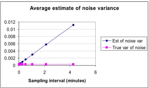
Recall that Theorem 1 also indicates that a rescaled version of the quadratic variation estimator
should converge to the variance of the noise process. Fig. 5 represents the rescaled realized volatility,
namely Vbi
M, for different sampling frequencies and a value of the ratio between variance of the noise
process and underlying quadratic variation equal to 0.0284%. As earlier, the sampling interval (in
minutes) is given on the horizontal axis. The horizontal line in the plot is now the true variance of
the noise process. Clearly, the rescaled realized volatility estimates converge to the second moment
of the contaminations-in-return ε0s as the sampling interval goes to zero (i.e., as the number of
observations M increases without bound). We perform the same exercise with sample averages of
fourth powers of the contaminated return data for a variety of sample frequencies (see Fig. 6).
Again, we confirm the validity of the predictions contained in Theorem 2.
5.3
The biases in the quarticity estimates and their impact on the
con-ditional MSE of the realized volatility estimator: simulations based
on IBM.
In this subsection we show that alternative (but credible) sampling frequencies used to compute
the underlying quarticity (i.e., the remaining input in Eq. (30)) have little impact on the sampling
distribution of the optimal number of observations needed to calculate the object of interest, i.e.,
the underlying quadratic variation of the log price process. In addition, we show that, when the
quarticity is estimated relatively accurately, the rule-of-thumb in Lemma 4 delivers a distribution
of the estimated optimal sampling frequencies that is similar to the distribution obtained from the
full minimization of the conditional MSE. Should the quarticity be estimated imprecisely, then the
rule-of-thumb would deliver estimates that are more biased and considerably more volatile then
those delivered by the full minimization.
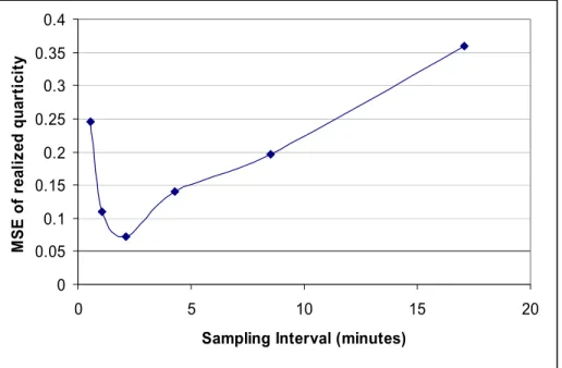
In Fig. 7 we plot the empirical MSE of the realized quarticity. The minimum is around 2
minutes. Going from the 2−minute sampling frequency to the 15-minute sampling frequency implies multiplication of the MSE by a factor of 4. Interestingly, even though the loss would be considerable
should one be just interested in the estimation of the quarticity per se, we will show that the impact
of the suboptimal 15-minute frequency on the sampling distribution of the minima of the conditional
MSE of the realized volatility estimator is not substantial. In light of the attention that the recent
empirical literature has devoted to the 15-minute sampling interval (see Andersen et al. (2000),
for instance), this observation will lead us to recommend the 15-minute sampling frequency for the
quarticity estimates as a valid frequency for stocks with various degrees of liquidity (see, also, Bandi
and Russell (2003b)). Naturally, as shown in Fig. 7, such choice is quite conservative for highly
liquid stocks like IBM. We will return to these important remarks.
In Fig. 8 we plot the distribution (across the 1,000 simulations) of the optimal sampling
frequen-cies obtained by minimizing the expression in Eq. (22) for values of the quarticity estimates obtained
by sampling at the correct 2-minute interval. Some observations are in order. First, despite the
exis-tence of an upward bias in the estimated values (the mean and the median are equal to 2.8 minutes
while the true optimal frequency is 1.7 minutes) the range of possible values is very informative
about the magnitude of the optimal frequency. For instance, the obtained range does not include
the 5-minute interval that has been largely used in the empirical work on the subject. Second, the
bias goes in the right direction in the sense that it provides us with a conservative assessment of the
optimal sampling interval while keeping us away from high frequencies corresponding to the upward
spike in the MSE of the realized volatility estimator. Finally, for the range of values in Fig. 8, the
incremental impact of lowering the sample frequency on the MSE of the realized volatility estimator
is rather small. The value of the MSE at the optimal 1.7-minute frequency is.014.It is 0.0143 at the
2 minute interval and 0.016 at the 3.5-minute frequency. At the 5-minute interval, the MSE value
is virtually twice as large as the corresponding value at the 2-minute interval (.027). Admittedly,
these considerations are conditional on choosing a frequency for the quarticity that is very close to
the optimal value as suggested by the simulated MSE for the quarticity in Fig. 7.
Thus, in Fig. 9 we report the distribution of the optimal frequencies for values of the quarticity
that are estimated using a 15-minute interval. The incremental bias is minimal. Additionally, while
the increased variance in the quarticity estimates (as testified by the MSE in Fig. 7) translates into
increased dispersion of the optimal frequencies, the array of possible values is still very informative
about the range of acceptable frequencies. In other words, using an inaccurate measure of the
underlying quarticity does not entail an uninformative characterization of the optimal sampling
employing a 15-minute frequency for the quarticity is a conservative choice. While it was shown that
such choice produces informative estimates, it can certainly be improved upon. In effect, our results suggest that it believable that higher (than 15 minutes) sampling frequencies would be appropriate
in the case of very liquid stocks (like IBM). Having said this, we think that a 15-minute sampling
interval for the quarticity estimates provides sufficient information about the optimal sampling interval (Bandi and Russell (2003b) confirm this finding). Furthermore, it is an easy interval to
use. Therefore, it deserves attention in applied work. Coherently, the 15-minute frequency is the
frequency that we utilize in the empirical application in next subsection.
For completeness, we also report results for the case where the quarticity is computed using
a sampling frequency equal to 30 minutes (see Fig. 10). While the increase in the bias is not
considerable, the likelihood of obtaining large values is substantially higher than in the previous
case. In effect, there is a non-negligible probability of obtaining optimal sampling frequencies in excess of 5 minutes. Nonetheless, the implied frequencies are still quite informative. For instance,
ourfindings clearly rule out frequencies that have been put forward as sensible conjectures in the
presence of microstructure noise in the empirical literature on the subject, namely frequencies in
the vicinity of the 15-minute interval (the maximum value across the 1,000 simulations is equal to
11.6 minutes). To conclude, even though we do not recommend using a 30-minute sampling interval
for the quarticity, wefind it reassuring that possibly very volatile estimates for it (as determined by
very suboptimal choices of the corresponding frequency) do not cause equally suboptimal sampling
frequencies for the realized volatility estimates.
In Figs. 11 through 13 we examine the impact of various quarticity measurements on the
distribu-tions on the optimal sampling frequencies for the realized volatility estimator obtained by employing
the rule-of-thumb in Lemma 4. Wefind that the estimates are more upward biased and variable than
in the case where a full minimization of the conditional MSE is performed. While these results hold
across different choices of the quarticity estimates, they are particularly pronounced as we move to highly suboptimal choices of the optimal sampling frequency for the quarticity. In effect, the approx-imation that is provided by Lemma 4 above appears very valid when a close-to-optimal frequency
for the quarticity is chosen (see Fig. 11). When using a 15-minute frequency for the quarticity, for
instance, the estimates that the approximation provides are considerably more variable than in the
full minimization case (since values as high as 20 minutes are possible). Nonetheless, the distribution
sampling frequency. In effect, due to the evident right skewness in the simulated distribution, the likelihood of obtaining values around 2 minutes (i.e., near the true optimal frequency) is about 50%.
In Figs. 14 and 15 we plot the true conditional MSE as implied by Eq. (22) above and
corre-sponding 95% bands based on the simulations. In light of our previous remarks, in both cases we use
the conservative 15-minute interval to estimate the underlying quarticity and quadratic variation.
Coherently with the average arrival time for a new price quote for the stock IBM in the month of
February 2002, in Fig. 14 we employ a 10 second sampling interval to estimate the necessary features
of the noise process (i.e., the second and the fourth moment). A 1 second sampling interval for the
same objects is used in Fig. 15. As expected, the graphs show that the estimated conditional MSE
expansion is more accurate when using moments of the noise process that are defined on the basis
of very high frequencies. This result is understandable in that higher frequencies lead to more
pre-cise estimates of the noise characteristics. Hence, stocks whose price updates occur very frequently
should lead to extremely accurate MSE expansions.
5.4
Computing the optimal frequency for IBM.
In Fig. 16 we plot the estimated conditional MSE of IBM along with the minimum from the full
minimization as implied by Eq. (30) and the minimum from the rule-of-thumb reported in Eq. (31).
The realized quarticity is estimated conservatively (see the previous subsection) using the 15-minute
sampling interval. We employ the high frequency quote-to-quote price changes to calculate the
moments of the noise process.
Several observations are in order. First, the optimal sampling interval is equal to 1.5 minutes.
This interval is shorter than the 5-minute interval that is used in some empirical work on the subject
(see Andersen et al. (2001), for instance). Consequently, it is shorter than recent conjectures on
optimal sampling based on the 15/20 minute interval (see Andersen et al. (2000)). Nonetheless, this
result crucially hinges on the liquidity features of the stock. Bandi and Russell (2003b) find that
less liquid stocks than IBM require lower sampling frequencies leading to optimal intervals that are
in the vicinity of the 5-minute interval.
Second, the loss that is induced by suboptimal sampling depends on the slope of the conditional
MSE. Going from the optimal frequency of 1.5 minutes to the 15-minute interval almost doubles the
MSE. This effect is economically important since the magnitude of the MSE is large. One can easily have a feel for it by a straightforward comparison of the root MSE (as implied by the values on
the horizontal axis of Fig. 16) and the average realized volatility, namely.0273%.At the 15-minute
interval the ratio between the two quantities is equal to about 36%. An alternative way to assess the
importance of accounting for microstructure contaminations in returns when estimating volatility
using high frequency data is to compare the magnitude of the MSE expansion to the variance that
would emerge from models that do not explicitly allow for noise (BN-S (2002, 2004), for instance).
In the case of IBM wefind that the value of the squared bias alone is larger than the value of the
variance term.
Finally, we notice that the rule-of-thumb in Lemma 4 provides an empirical answer to the optimal
frequency problem that is almost indistinguishable from the answer that is provided by the full
minimization of the expansion in Eq. (22). More precisely, we find that the approximate optimal
frequency is 1.45. After one takes into consideration that the quality of the approximation is higher in
the presence of a large number of observationsM(see Section 4) and that the theoretical dispersion of
the approximate estimates can be high (see the previous subsection), the rule-of-thumb can provide
very useful and immediate implications for empirical work. Bandi and Russell (2003b) confirm this
finding for a variety of S&P100 stocks.
6
Conclusions
Recorded prices are known to diverge from their “efficient” values due to the presence of market microstructure contaminations.
We find that the presence of market microstructure noise in high-frequency data makes the
consistent estimation of the quadratic variation of the underlying log price process through the
con-ventional realized volatility estimator unachievable. In effect, the summing of increasingly-frequent contaminated return data simply entails infinite accumulation of noise. Interestingly, we point out
that a standardized version of the realized volatility estimator can be employed to consistently
esti-mate the second moment of the unobservable noise process. More generally, we stress that sample
averages of powers of contaminated returns converge to the moments of the underlying noise process.
Moving from asymptotic arguments to finite sample results, we argue that the microstructure
noise creates a dichotomy in the model-free estimation of integrated volatility. While it is
theoreti-cally necessary to sum squared returns that are computed over very small intervals to better identify
the underlying volatility over a period, the summing of numerous contaminated return series entails
bias/variance trade-off. We quantify the trade-offin the presence of a realistic model of price deter-mination and discuss optimal sampling (for the purpose of volatility estimation) on the basis of the
(estimable) moments of the distribution of the noise process and the underlying quarticity of the log
price process.
Specifically, in the spirit of the simplicity and generality of the conventional realized volatility
estimator as a nonparametric measurement of the quadratic volatility of the underlying log price
process, we derive simple implications and tools for empirical work on quadratic volatility estimation
through realized volatility. We summarize ourfindings as follows.
(1) The optimal sampling problem can be written as the minimization of the conditional MSE
expansion of the realized volatility estimator.
(2) The main ingredients of the MSE expansion are the second and the fourth moment of the
(unobserved) noise process and the so-called quartic volatility of underlying log price process.
(3) We show that the moments of the underlying noise process can be estimated consistently in the
presence of high frequency observations. Even though the quarticity estimator (as suggested by
BN-S (2002)) does not provide a consistent nonparametric estimate of the remaining ingredient
of the MSE expansion, i.e., the quartic volatility, if noise plays a role, we stress that alternative
(plausible) choices of sampling frequency for it do not have a substantial impact on the optimal
sampling of the realized volatility estimator.
(4) More precisely, we deem the (easy to implement) 15-minute sampling interval to be a valid
(albeit conservative) choice of frequency for the quarticity estimator. Such choice can be
improved upon (i.e., lowered) in the case of very liquid stocks.
(5) In addition to providing a straightforward minimization program to solve, we offer a simple rule-of-thumb to select the optimal sampling frequency on the basis of an expression that could
be readily interpreted as a signal-to-noise ratio, namely the ratio between the quarticity of the
log price process and the second moment of the unobserved noise.
Despite having the property of delivering more variable estimates of the optimal frequency
that the full minimization, the rule-of-thumb can provide a very useful preliminary assessment
very accurate when the true optimal sampling frequency is high and the quarticity is estimated
accurately.
An application of our methodology to a liquid stock like IBM points to the necessity of a sampling
interval that is smaller that intervals typically employed in applied work on the subject. Furthermore,
our analysis provides the following conclusions:
(1) Properly accounting for market microstructure effects suggests that the MSE can be large relative to the realized volatility estimates.
(2) An MSE that fails to account for market microstructure noise can substantially understate the
true MSE.
(3) Failing to sample at the optimal frequency can lead to large inefficiencies in the quality of the realized volatility estimates.
Onefinal observation is needed. The present paper suggests a simple nonparametric technique
to learn about features of the noise component in recorded high-frequency asset prices as well as
about the genuine volatility properties of the efficient prices. As such, it provides tools that might prove useful in two separate strands of thefinance literature, namely empirical microstructure and, of
course, volatility estimation. The importance of the later is apparent. Here, we briefly expand on the
former. A considerable amount of work has been devoted to understanding the determinants of the
quoted bid-ask spreads. Nonetheless, it is well-known that the (average) between the bid and the ask
quotes are imprecise measurements of the true cost of trade in that transactions often occur within
the posted spreads. In consequence, the true quantity of interest is the so-called “effective spread,” namely the difference between the transaction price and the efficient price. When using transaction prices rather than mid-point bid-ask quotes as in this paper, the methods proposed in the present
piece can be used to provide nonparametric measurements of the (unconditional) distributional
features of the effective spreads. Such features can be put to work to investigate the cross-sectional determinants of the implicit cost-of-trade as in Bandi and Russell (2003c) . Alternatively, one can
modify the set-up that was previously discussed in order to allow for heteroskedastic structures in
the noise process and study the dynamic features of the estimated microstructure frictions. The
time series dynamics are currently being studied by the authors and will be reported in Bandi and
7
Appendix A: Proofs
Proof of Lemma1. E(ε2) = E(η−η−1)2 (34) = E¡η2−2ηη−1+η2−1¢ (35) = 2σ2η. (36) E¡ε4¢ = E¡η−η−1¢4 (37) = E¡η2−2ηη−1+η2−1¢2 (38) = E(η4−2η3η−1+η2η2−1) +E(−2η3η−1+ 4η 2 η2−1−2ηη 3 −1) +E(η2η2−1−2ηη 3 −1+η 4 −1) (39) = 2E¡η4¢+ 6σ4η. (40) E(ε2ε2−1) = E £ (η−η−1) 2 (η−1−η−2) 2¤ (41) = E£(η2+η−21−2ηη−1)(η 2 −1+η 2 −2−2η−1η−2) ¤ (42) = E£η2η2−1+η 2 η2−2−2η 2 η−1η−2 ¤ +E£η4−1+η2−1η2−2−2η3−1η−2¤ −E£2ηη3−1+ 2ηη−1η2−2−4ηη2−1η−2¤ (43) = 3σ4η+E ¡ η4¢.¥ (44)Proof of Theorem 1. We study the term Ai first. The interested reader is referred to BN-S (2002)
for a different proof. Specifically, we generalize the classical BN-S result along two dimensions, namely we provide a functional central limit theorem-based argument and allow for leverage effects. Recall that h
δ =M and write Ai= h/δ X j=1 r2j,i= h/δ X j=1 ÃZ (i−1)h+jδ (i−1)h+(j−1)δ σsdWs !2 . (45) and Lij= Z (i−1)h+jδ 0 σsdWs. (46) Then, Ai = h/δ X j=1 ³ Lij−L i j−1 ´2 (47) = h/δ X j=1 µ³ Lij ´2 +³Lij−1 ´2 −2LijL i j−1 ¶ (48) = h/δ X j=1 µ³ Lij ´2 −³Lij−1 ´2 −2Lij−1 ³ Lij−L i j−1 ´¶ . (49)
Now, we note that
³ Lij ´2 = Ã Li0+ 2 Z (i−1)h+jδ 0 LidLi ! +hLii (i−1)h+jδ (50)
by the Doob’s decomposition (see Theorem 4.7 in Chung and Williams (1990), for instance). It is known that ³ Li0+ 2 R(i−1)h+jδ 0 L i
dLi´is a continuous local martingale whereas£Li¤(i
−1)h+jδ is a continuous increasing process with initial value zero, i.e., the quadratic variation of the local martingaleLi between time 0 and time (i−1)h+jδ. Then, Ai= h/δ X j=1 Ã 2 Z (i−1)h+jδ (i−1)h+(j−1)δ LidLi+hLii j−1,j− 2Lij−1 ³ Lij−L i j−1 ´! , (51) where h Lii j−1,j =hLii (i−1)h+jδ− h Lii (i−1)h+(j−1)δ = Z (i−1)h+jδ (i−1)h+(j−1)δ σ2sds. (52) Hence, Ai= h/δ X j=1 h Lii j−1,j + 2 h/δ X j=1 Z (i−1)h+jδ (i−1)h+(j−1)δ ³ Li−Lij−1 ´ dLi (53) and Ai− Z ih (i−1)h σ2sds= 2 h/δ X j=1 Lj−1,j, (54) where Lj−1,t= Z (i−1)h+tδ (i−1)h+(j−1)δ ³ Li−Lij−1 ´ dLi j−1≤t≤j (55)
is a continuous local martingale with zero mean. Now, write
ΦMt := 2 r M h h/δ−1 X j=1 Lj−1,j+ Z (i−1)h+tδ (i−1)h+(h δ−1)δ ³ Li−Lih δ−1 ´ dLi , (56) with h δ −1< t≤ h δ, whereΦ M
t is a continuous local martingale with (limiting) increasing process
£
ΦM¤ t
4M h h/δ−1 X j=1 Z (i−1)h+jδ (i−1)h+(j−1)δ ³ Li−Lij−1 ´2 dhLii+ 4M h Z (i−1)h+tδ (i−1)h+(h δ−1)δ ³ Li−Lih δ−1 ´2 dhLii a ∼4M h h/δ−1 X j=1 Z (i−1)h+jδ (i−1)h+(j−1)δ h Li−Lij−1 i dhLii+ Z(i−1)h+tδ (i−1)h+(hδ−1)δ h Li−Lih δ−1 i dhLii (57) = 4M h( h/δ−1 X j=1 Z (i−1)h+jδ (i−1)h+(j−1)δ h Li−Lij−1 i dhLi−Lij−1 i + Z (i−1)h+tδ (i−1)h+(h δ−1)δ h Li−Lih δ−1 i dhLi−Lih δ−1 i ) (58) = 4M h h/δ−1 X j=1 £ Li −Li j−1 ¤2 2 | j j−1+ h Li−Lih δ−1 i2 2 | t h δ−1 (59) = 2M h h/δ−1 X j=1 h Lij−L i j−1 i2 +hLit−L i h δ−1 i2 (60) = 2M h h/δ−1 X j=1 ÃZ (i−1)h+jδ (i−1)h+(j−1)δ σ2ds !2 + ÃZ (i−1)h+tδ (i−1)h+(h δ−1)δ σ2ds !2 . (61)
We now define the stopping timesτ= inf©s:£ΦM¤
s> t
ª
.Hence,Bt=ΦMτ is a=τ-Brownian motion and
ΦMt =B[ΦM] t
is the so-called DDS (Dambis, Dubins-Schwartz) Brownian motion ofΦt (see Revuz and Yor (Theorem 1.6, 1994)). Finally, r M h " Ai− Z ih (i−1)h σ2sds # = ΦMh/δ ⇒ M→∞B 2M h h/δ X j=1 ÃZ (i−1)h+jδ (i−1)h+(j−1)δ σ2sds !2 (62) d =B Ã 2 ÃZ ih (i−1)h σ4sds !! , (63) where Qi = Rih (i−1)hσ 4
sds is the quartic variation (over h) as defined in BN-S (2002), by the asymptotic
Knight’s theorem (see Revuz and Yor (Theorem 2.3, 1994)). Under Assumption 1(3), i.e., absence of leverage effects, we can write
B Ã 2 ÃZ ih (i−1)h σ4sds !! d =MN Ã 2 ÃZ ih (i−1)h σ4sds !! . (64)
This proves the result in Remark 1. We now study the termBi, that is h/δ
X
j=1
ε2j,i. (65)
A conventional central limit theorem for stationary mixing sequences (see Hamilton (1994), for example) allows us to write