University of Mississippi University of Mississippi
eGrove
eGrove
Electronic Theses and Dissertations Graduate School
2016
On Variable Bandwidth Kernel Density And Regression Estimation
On Variable Bandwidth Kernel Density And Regression Estimation
Janet Nakarmi
University of Mississippi
Follow this and additional works at: https://egrove.olemiss.edu/etd
Part of the Statistics and Probability Commons
Recommended Citation Recommended Citation
Nakarmi, Janet, "On Variable Bandwidth Kernel Density And Regression Estimation" (2016). Electronic Theses and Dissertations. 678.
https://egrove.olemiss.edu/etd/678
ON VARIABLE BANDWIDTH KERNEL DENSITY AND REGRESSION ESTIMATION DISSERTATION
A Dissertation
presented in partial fulfillment of requirements for the degree of Doctor of Philosophy
in the Department of Mathematics The University of Mississippi
by
JANET NAKARMI August 2016
ABSTRACT
We study the ideal variable bandwidth kernel density estimator introduced by McKay [16, 17] and the plug-in practical version of the variable bandwidth kernel density estimator with two sequences of bandwidths as in [10]. We estimate the variance of the variable bandwidth kernel density estimator. Based on the exact formula of the bias and the variance of the variable bandwidth kernel density estimator, we develop the optimal bandwidth selection of the true variable bandwidth kernel density estimator. Furthermore, we present the central limit theorem of the true variable bandwidth kernel density estimator. We also propose a new variable bandwidth kernel regression estimator and estimate the bias and propose the central limit theorems for its ideal and true versions.
For the one dimensional case, the order of the bias and variance is same for the vari-able bandwidth kernel density estimator and for the proposed varivari-able bandwidth kernel regression estimator. Since we use the order of the bias and variance to find the optimal bandwidth, the optimal bandwidth for these estimators are also the same. Comparing the integrated mean square error of the variable bandwidth kernel density estimator (the vari-able bandwidth kernel regression estimator) with the classical kernel density estimator (the Nadaraya-Watson estimator), we find that the variable bandwidth kernel estimators have a faster rate of convergence. Furthermore, we prove that these variable bandwidth kernel estimators converge to normal distribution.
DEDICATION
This dissertation is dedicated to my parents Narayan Lal and Purna Laxmi Nakarmi. Without their support, love and encouragement, I would not have been able to come this
far. I would also like to dedicate this work to my best friend, Himani Vaidya for being there for me throughout the entire graduate program.
ACKNOWLEDGEMENTS
I would like to thank my advisor Dr. Hailin Sang for his continuous support, patience and vast knowledge. His guidance throughout the whole process of writing this dissertation has helped me immensely. I could not have imagined having a better advisor for my Ph.D research.
Besides my advisor, I would also like to thank Dr. Xin Dang, Dr. Erwin Mi˜na Diaz, Dr. Yixin Chen, and Dr. Martial Longla for their insightful comments and for giving their time to serve on my committee. I would like to thank Dr. James Reid for his support and vast knowledge in LaTeX. A special thanks goes to Dr. Kayla Harville, Colleen Gilman, Casandra Jenkins, Shelia Lewis, and Kay Phillips, who were always there to help and encourage me anytime that I needed it. I greatly appreciate the support of the entire Department of Mathematics and cherish the friendship and support that I have received from all of its members.
TABLE OF CONTENTS
ABSTRACT . . . ii
DEDICATION . . . iii
ACKNOWLEDGEMENTS . . . iv
List of Figures . . . vii
1 INTRODUCTION . . . 1
1.1 CLASSICAL KERNEL DENSITY ESTIMATOR . . . 1
1.2 VARIABLE BANDWIDTH KERNEL DENSITY ESTIMATOR . . . 2
1.3 KERNEL-TYPE REGRESSION ESTIMATOR . . . 4
1.4 VARIABLE BANDWIDTH KERNEL REGRESSION ESTIMATOR . . . . 6
1.5 OVERVIEW . . . 7
1.5.1 Contribution of the dissertation . . . 7
1.5.2 Structure of the Dissertation . . . 8
2 VARIABLE BANDWIDTH KERNEL DENSITY ESTIMATION . . . 9
2.1 DECOMPOSITION FOR KERNEL DENSITY ESTIMATION . . . 9
2.2 BIAS OF VARIABLE BANDWIDTH KERNEL DENSITY ESTIMATOR . 12 2.2.1 Notations and Assumptions . . . 12
2.3 VARIANCE OF VARIABLE BANDWIDTH KERNEL DENSITY
ESTIMA-TOR . . . 18
2.3.1 Ideal Estimator . . . 18
2.3.2 True Estimator in One Dimension . . . 22
2.4 CENTRAL LIMIT THEOREM FOR VARIABLE BANDWIDTH KERNEL DENSITY ESTIMATOR . . . 34
2.4.1 Ideal Estimator . . . 34
2.4.2 True Estimator . . . 36
2.5 OPTIMAL BANDWIDTH AND SIMULATION ON VARIABLE BANDWIDTH KERNEL DENSITY ESTIMATOR . . . 43
2.5.1 Optimal Bandwidthh∗2,n on Variable Bandwidth Kernel Density Esti-mation . . . 43
2.5.2 Simulation on Variable Bandwidth Kernel Density Estimation . . . . 44
3 VARIABLE BANDWIDTH KERNEL REGRESSION ESTIMATION . . . 46
3.1 DECOMPOSITION FOR KERNEL REGRESSION ESTIMATION . . . 46
3.2 BIAS OF VARIABLE BANDWIDTH KERNEL REGRESSION ESTIMATOR 48 3.2.1 Ideal Estimator . . . 48
3.2.2 True Estimator . . . 54
3.3 CENTRAL LIMIT THEOREM FOR VARIABLE BANDWIDTH KERNEL REGRESSION ESTIMATOR . . . 66 3.3.1 Ideal Estimator . . . 66 3.3.2 True Estimator . . . 70 4 CONCLUSION. . . 82 BIBLIOGRAPHY . . . 83 VITA . . . 86
LIST OF FIGURES
2.5.1 The probability density functions of t-distribution (t4(0,1)), Cauchy(0,1) and Pareto(0,1), the kernel density estimates (KDE), and the variable kernel den-sity estimates (VKDE) with 50,000 observations generated from t-distribution (t4(0,1)), Cauchy(0,1) and Pareto(0,1) distribution. The left one shows the estimate in the main area with the mode. The right one shows the estimate in the tail area. . . 45
1 INTRODUCTION
1.1 CLASSICAL KERNEL DENSITY ESTIMATOR
Suppose thatXi, for i= 1,· · · , n, n∈N, are independent and identically distributed
(i.i.d.) observations with density function f(t), t ∈ Rd. The goal of nonparametric density
estimation is to estimate f with as few assumptions about f as possible. One of the well known estimators of f is the classical kernel density estimator, which we will denote by
ˆ f(t;hn) = 1 nhd n n X i=1 K t−Xi hn , (1.1.1)
wherehnis the bandwidth sequence satisfying hn→0, nhdn → ∞and K is a kernel function.
A kernel function,K, is any function that satisfiesR
K(x)dx= 1. The kernelK satisfies the following conditions to get the order of the bias and variance of the classical kernel density estimator: K(x) ≥ 0, R xK(x)dx = 0, and σ2 K = R x2K(x)dx > 0. The variance of (1.1.1) has order O((nhd n)
−1) and the bias has order O(h2
n) when f(t) has bounded second order
partial derivatives. See [25] and [27] for the literature on kernel density estimation. Throughout this dissertation we use the following definitions and notations.
Definition 1.1.2. I) an=o(bn) iff an/bn→0.
II) an =O(bn) iff there exists constants S and n0 such that |an| ≤Sbn for n≥n0.
III) Xn = Op(an) iff for every > 0 there exists constants C and n such that P(|Xn| ≤
V) Xn = Oa.s(an) iff there exists a constant B such that |Xn| ≤ Ban a.s. for n large
enough.
VI) Xn =oa.s(an) iff there exists a sequence δn→0 such that |Xn| ≤δnan a.s.
1.2 VARIABLE BANDWIDTH KERNEL DENSITY ESTIMATOR
We study the following multidimensional version of the variable bandwidth kernel density estimator proposed in [16] and [17]:
¯ f(t;hn) = 1 nhd n n X i=1 αd(f(Xi))K(h−n1α(f(Xi))(t−Xi)), (1.2.1) with α(s) := cp1/2(s/c2), (1.2.2) where c is a fixed number with 0 < c < ∞ and the function p has at least fourth order
derivative and satisfies the following conditions:
p(x)≥1 for allx∈R, (1.2.3)
p(x) =x for all x≥t0 for some 1≤t0 <∞. (1.2.4)
The study of variable bandwidth kernel density estimation goes back to [1]. Abramson [1] proposed the estimator
fA(t;hn) = 1 nhd n n X i=1 γd(t, Xi)K(h−n1γ(t, Xi)(t−Xi)), (1.2.5)
where γ(t, s) = (f(s)∨f(t)/10)1/2. The true bandwidth, h
n/γ(t, Xi), at each observation Xi is inversely proportional to f1/2(Xi) if f(Xi) ≥ f(t)/10 (which is the square root law).
Notice that (1.2.1) also has the square root law since α(f(Xi)) = f1/2(Xi) if f(Xi) ≥
hn/γ(t, Xi)≥101/2hn/f(t)1/2. The clipping procedures prevent too much contribution to the
density estimation at t if the observation Xi is too far away from t. Abramson showed that this square root law and the clipping procedure improve the bias from the order ofh2n to the order of h4
n for the estimator (1.2.5), while at the same time keep the variance at the order
of (nhd n)
−1 if f(t) 6= 0 and f(t) has fourth order continuous derivatives at t. However, this
variable bandwidth estimator (1.2.5) is not a density function since the integral of fA(t;hn)
over t is not 1.
Terrell & Scott [26] and McKay [17] showed that a modification of the Abramson estimator without the ‘clipping filter’ (f(t)/10)1/2 onf1/2(Xi) studied in [13], namely,
fHM(t;hn) = 1 nhd n n X i=1 fd/2(Xi)K(h−n1f 1/2(X i)(t−Xi)), (1.2.6)
which has integral 1 and thus is a true probability density, may have bias of order much larger than h4n. Therefore, the clipping is necessary for bias reduction. In the case d = 1,
Hall et al. [12] proposed the estimator
fHHM(t;hn) = 1 nhn n X i=1 K t−Xi hn f1/2(Xi) f1/2(Xi)I(|t−Xi|< hnB), (1.2.7)
where B is a fixed constant. This estimator is non-negative and achieves the desired bias reduction but, like Abramson’s estimator, it does not integrate to 1. See also [21] for a similar estimator.
In conclusion, it seems that the estimator (1.2.1) has all the advantages: it is a true density function with square root law and smooth clipping procedure. However, notice that this estimator and all the other variable bandwidth kernel density estimators are not applicable in practice since they all include the studied density function f. They are called ideal estimators in the literature. Hall & Marron [13] studied the true density estimator
ˆ f (t;h , h ) = 1 n X K t−Xi ˆ f1/2(X;h ) ˆ fd/2(X;h ),
by plugging in a pilot estimator, the classical estimator (1.1.1), into the estimator (1.2.6). They used the Taylor expansion ofK
t−Xi h2,n ˆ f1/2(Xi;h1,n) atK t−Xi h2,n f 1/2(Xi)to prove that the difference between the true estimator ˆfHM(t;h1,n, h2,n) and the ideal version (1.2.6) has
pointwise asymptotic convergence rate OP(n−4/(8+d)). By applying this Taylor
decomposi-tion, McKay [17] studied convergence in probability and pointwise of plug-in true estimator of (1.2.1). Gin´e & Sang [9, 10] studied plug-in true estimators of (1.2.7) and (1.2.1) for one and d-dimensional observations. They proved that the difference between the true estimator and the true value (f(t)) converges uniformly over a data adaptive region at the rate of
Oa.s.((logn/n)4/(8+d)) by applying empirical process techniques. The true estimator in [10]
has the following form:
ˆ f(t;h1,n, h2,n) = 1 nhd 2,n n X i=1 K t−Xi h2,n α( ˆf(Xi;h1,n)) αd( ˆf(Xi;h1,n)). (1.2.8)
Jones et al. [15] studied ideal estimators with bias order h6
n. The ideal estimators studied
in [15] achieved bias reduction by adapting the bandwidth about each Xi to the size of f(Xi), with smooth clipping for small values of f(Xi), and using concentrated kernels, in
order to keep the estimators local. Samiuddin & El-Sayyad [23] achieved the same results by shifting the centers of the windows by random quantities. Gin´e & Sang [10] studied the uniform convergence in almost sure sense of the true estimators corresponding to these ideal estimators.
1.3 KERNEL-TYPE REGRESSION ESTIMATOR
Suppose (X1, Y1), ...,(Xn, Yn) are n pairs ofi.i.d.observations, where Y1 is a bounded random variable. Xi, Yi ∈ R, f is the probability density function of X1, and r is the
regression function defined as the conditional mean of Y:
We want to estimate r(t) using (X1, Y1), ...,(Xn, Yn). One commonly used nonparametric
regression estimator for r(t) was introduced independently by Nadaraya [19] and Watson [28]. The so called Nadaraya-Watson estimator is defined as
ˆ r(t;hn) = Pn i=1K t−Xi hn Yi Pn i=1K t−Xi hn = 1 nhn Pn i=1K t−Xi hn Yi 1 nhn Pn i=1K t−Xi hn = ˆ g(t;hn) ˆ f(t;hn). (1.3.2)
Iff(t) andr(t) have bounded second order derivatives and the random variableY is bounded, then the bias has order O(h2
n) and the variance of (1.3.2) has order O((nhn)−1). The proof
of the bias of the Nadaraya-Watson estimator, (1.3.2), can be found in both [4] and [22]. Noda [20] established the convergence of the Nadaraya-Watson estimator to r(t) and the mean square error at a continuous point. He also proved the consistency of estimator ˆg(t;hn) f(t)
almost surely whenf(t) known. The uniform consistency of the Nadaraya-Watson estimator was shown in [2] for the case of discrete Xi0s. See [27] and [24] for more literature on the Nadaraya-Watson estimator.
Einmahl & Mason [6, 7] studied the estimator
ˆ rn(t, q) = Pn i=1K t−Xi hn q(Yi) nhnfˆ(t, hn) , (1.3.3)
whereqis a chosen measurable function, for the regression functionr(t, q) :=E(q(Y)|X =t).
Notice that for q(Y) = Y, we get the regression function (1.3.1). Einmahl & Mason [6] obtained the exact results for the rate of uniform consistency of regression estimators with some additional smoothness conditions for t in a compact interval. The rate of uniform consistency of the regression estimators was of orderOa.s.(pnhn|loghn|).
1.4 VARIABLE BANDWIDTH KERNEL REGRESSION ESTIMATOR
Defineg(t) :=r(t)f(t). Considerα(x) defined by (1.2.2) and then we haveα(g(t)) by
α(g(t)) =α(r(t)f(t)). (1.4.1)
We propose and study the following version of the variable bandwidth kernel regression estimator: ¯ r(t;hn) = Pn i=1K t−Xi hn α(g(Xi)) α(g(Xi))Yi Pn i=1K t−Xi hn α(f(Xi)) α(f(Xi)) (1.4.2) = 1 nhn Pn i=1K t−Xi hn α(g(Xi)) α(g(Xi))Yi 1 nhn Pn i=1K t−Xi hn α(f(Xi)) α(f(Xi)) = g¯¯(t;hn) f(t;hn) . (1.4.3)
One of the few studies on variable bandwidth kernel regression estimators was done by M¨uller & Stadtm¨uller [18]. They introduced the following variable bandwidth kernel estimator for regression curve:
ˆ r(t;ht) = 1 nht n X i=1 K t−xi ht Yi, (1.4.4)
for a given function t → ht, t ∈ [0,1]. For r(t) ∈ Ck[0,1] (we say that a function r is in
Ck[0,1] if it and its first k derivatives are bounded and uniformly continuous on [0,1]), the optimal bandwidth forhthas the order ofO(n−1/(2k+1)). To estimate the regression function r(t) in (1.3.1), M¨uller & Stadtm¨uller [18] worked on variation of bandwidth depending on t
whereas we study bandwidth depending on the sample. Einmahl & Mason [7] also worked on establishing consistence of kernel-type estimators (1.3.3) in the multidimensional case when the bandwidthhn is a function of the locationt or the data. We will study the true variable
ˆ rn(t;h1,n, h2,n) = Pn i=1K t−Xi h2,nα(ˆg(Xi;h1,n)) α(ˆg(Xi;h1,n))Yi Pn i=1K t−Xi h2,nα( ˆf(Xi;h1,n)) α( ˆf(Xi;h1,n)) = 1 nh2,n Pn i=1K t−Xi h2,nα(ˆg(Xi;h1,n)) α(ˆg(Xi;h1,n))Yi 1 nh2,n Pn i=1K t−Xi h2,n α( ˆf(Xi;h1,n)) α( ˆf(Xi;h1,n)) = ˆg(t;h1,n, h2,n) ˆ f(t;h1,n, h2,n) , (1.4.5) where ˆg(t;h1,n) = ˆr(t;h1,n) ˆf(t;h1,n). 1.5 OVERVIEW
1.5 Contribution of the dissertation
The contribution of this dissertation is as follows:
• We showed that the optimal bandwidth of the true variable bandwidth kernel density
estimator is of the formJ n−1/(8+d), for some finite constant J.
• We have established central limit theorems for the ideal and true variable bandwidth
kernel density estimators.
• We have extended the ideal and true variable bandwidth kernel density estimators to
kernel regression.
• We have estimated the bias for both the ideal and true variable bandwidth kernel
regression estimators.
• We have found the asymptotic variance for the ideal and true variable bandwidth kernel
regression estimators.
1.5 Structure of the Dissertation
This dissertation is organized in the following way. In Section 2 of Chapter 2 and Section 3.1 of Chapter 3 we discuss the expansion of functions Kt−Xi
h2,nα( ˆf(Xi;h1,n)) , α( ˆf(Xi;h1,n)), K t−Xi h2,nα(ˆg(Xi;h1,n))
, and α(ˆg(Xi;h1,n)). We will also assess the
conver-gence rate of the terms in the expansions. Section 2.2 focuses on the bias of the true variable bandwidth kernel density estimator in the multidimensional case. The variance of the ideal variable bandwidth kernel density estimator for the multidimensional case and the variance of the true variable bandwidth kernel density estimator for the one dimensional case are presented in Section 2.3. Section 2.4 provides central limit theorems for the ideal and true variable bandwidth kernel density estimators. Section 2.5 provides a simulation study and optimal bandwidth selection for the true variable bandwidth kernel density estimator. In Section 3.2 of Chapter 3, the bias of the ideal and true variable bandwidth kernel regres-sion estimators for the one dimenregres-sional case is estimated. Section 3.3 presents central limit theorems for the ideal and true variable bandwidth kernel regression estimators. Chapter 4 gives the conclusion.
2 VARIABLE BANDWIDTH KERNEL DENSITY ESTIMATION
2.1 DECOMPOSITION FOR KERNEL DENSITY ESTIMATION
For convenience, we adopt the notations of [10] for the Taylor expansion of
Kt−Xi h2,n α( ˆf(Xi;h1,n)) atKt−Xi h2,n α(f(Xi))
. For details, see [10]. PC denotes the set of all
probability densities on Rd that are uniformly continuous and are bounded by C <∞, and
PC,k denotes the set of densities onRd where their partial derivatives of orderk or lower are
bounded by C < ∞ and are uniformly continuous. We say that a function g is in Cl(Ω) if
it and its firstl derivatives are bounded and uniformly continuous on Ω. Defineδ(t) =δ(t, n) by the equation
δ(t) = α( ˆf(t;h1,n))−α(f(t)) α(f(t)) . (2.1.1) Then, α( ˆf(t;h1,n)) = α(f(t))(1 +δ(t)) (2.1.2) and |δ(t)| ≤Bc−2|fˆ(t;h1,n)−f(t)| (2.1.3)
for a constantB that depends only onpand forc >0. Although we study the asymptotics of the true estimator pointwise, the uniform asymptotic behavior of the quantityδ(·) is needed
in the latter analysis. Define
Note that for f ∈ PC,2 by (3.5) of [10], sup t∈Rd |b1(t;h1,n)|=O(h21,n), (2.1.4) and by [8], sup t∈Rd |D1(t;h1,n)|=Oa.s. s logn nhd 1,n ! . Denote s logn nhd 1,n +h21,n :=U(h1,n). (2.1.5) Then, we have by (3.6) of [10], sup t∈Rd |δ(t)|= sup t∈Rd |fˆ(t;h1,n)−f(t)|= sup t∈Rd |D1(t;h1,n) +b1(t;h1,n)|=Oa.s.(U(h1,n)) (2.1.6)
for f ∈ PC,2. By the definition ofδ(t), we also have,
δ(t) = α 0(f(t))[ ˆf(t;h 1,n)−f(t)] α(f(t)) + α00(η)[ ˆf(t;h1,n)−f(t)]2 2α(f(t)) (2.1.7)
where η =η(t, h1,n) ≥0 is between ˆf(t;h1,n) and f(t). Note that, since p ≥1 and when p0
andp00are uniformly bounded on [0,∞), we have|α00(η(t, h1,n))| ≤c−3Afor some constantA
which depends only on the clipping function p. It is also convenient to record the following expansion of αd( ˆf) implied by (2.1.2) and (2.1.6):
αd( ˆf(t;h1,n)) =αd(f(t))(1 +dδ(t)) +δ1(t). (2.1.8)
By (3.9) of [10], we have
Hence, by (2.1.3) and (2.1.6), kδ1k∞ =Oa.s.(kfˆn(·;h1,n)−f(·)k2∞) for f ∈ PC,2. Set L1(t) = d X i=1 tiKi0(t) and L(t) = dK(t) +L1(t), t∈Rd, (2.1.9)
where Ki0 denotes the partial derivative of K in the direction of the i-th coordinate, and ti
denotes thei-th coordinate oft ∈Rd. By symmetry and integration by parts, we notice that
L is a second order kernel. We say that M is a second order kernel if R
uM(u)du = 0 and R
u2M(u)du >0.
We then have the following Taylor expansion
K t−Xi h2,n α( ˆf(Xi;h1,n)) =K t−Xi h2,n α(f(Xi)) + d X j=1 Kj0 t−Xi h2,n α(f(Xi)) (t−Xi)j h2,n α(f(Xi))δ(Xi) +δ2(t;Xi), (2.1.10) where δ2(t, Xi) = d X j,`=1 Kj,`00 (ξ)(t−Xi)j(t−Xi)` 2h2 2,n α2(f(Xi))δ2(Xi), (2.1.11)
ξbeing a number between t−Xi
h2,nα(f(Xi)) and t−Xi h2,n α(f(Xi))(1+δ(Xi)). By the analysis (3.12) and (3.13) in [10], sup t,x∈Rd |δ2(t, x)|=Oa.s. kfˆ(·;h1,n)−f(·)k2∞ =Oa.s.(U2(h1,n)) (2.1.12)
for f ∈ PC,2. Therefore, by using the expansion (2.1.8) of αd( ˆf), the Taylor expansion
(2.1.10), and the notations L1 and L in (2.1.9), we get
ˆ f(t;h1,n, h2,n) = ¯f(t;h2,n) + 1 nhd 2,n n X i=1 L t−Xi h2,n α(f(Xi)) αd(f(Xi))δ(Xi) + 1 nhd 2,n n X i=1 " K t−Xi h2,n α(f(Xi)) δ1(Xi) +αd(f(Xi))δ2(t, Xi) +dL1 t−Xi h2,n α(f(Xi)) αd(f(Xi))δ2(Xi) # + 1 nhd 2,n n X i=1 " L1 t−Xi h2,n α(f(Xi)) δ(Xi)δ1(Xi) +dαd(f(Xi))δ(Xi)δ2(t, Xi) # + 1 nhd 2,n n X i=1 δ2(t, Xi)δ1(Xi). (2.1.13)
2.2 BIAS OF VARIABLE BANDWIDTH KERNEL DENSITY ESTIMATOR
2.2 Notations and Assumptions
Letv = (v1, . . . , vd)∈(N∪ {0})d. |v|=Pdi=1vi, Dv :=D v1 x1◦ · · · ◦D vd xd,v! =v1!· · ·vd! and τv = R Rdu v1 1 · · ·u vd
d K(u)du. Let the kernelK below the following assumptions which are
required throughout the chapter.
Assumptions 1. Suppose that the kernel K onRd is non-negative and has the formK(t) =
Φ(ktk2)for some positive real-valued even function Φ with uniformly bounded second
deriva-tive and with support contained in [0, T], T <∞.
We also give assumptions on clipping function pand density function f.
Define
Dr :={t ∈Rd :f(t)> r > t0c2,ktk<1/r}, r >0. (2.2.1)
Here, c and t0 are the constants that appear in the clipping function α in (1.2.2).
2.2 Ideal Estimator
Corollary 2.2.1. ([16, 17]) Let α(f(t)) = cp1/2(c−2f(t)) for some c > 0. Define f¯(t;h
n)
by equation (1.2.1). Then, under Assumptions 2 for the clipping function p and density
function f, Ef¯(t;hn) = f(t) + X |v|=4 τvDv(1/f)/v! h4n+o(hn4) =f(t) +O h4n (2.2.2) as hn→0, uniformly onDr. 2.2 True Estimator
Proposition 2.2.2. Let α(f(t)) =cp1/2(c−2f(t)) for some c >0, and define fˆ(t;h
1,n, h2,n)
by (1.2.8). Assume thatU(h1,n) = o(h22,n). Then, as h2,n →0, fort∈ Dr under Assumptions
1 for K and Assumptions 2 for p and f,
E( ˆf(t;h1,n, h2,n))−f(t) = X |v|=4 τvDv(1/f)/v! h42,n+o(h42,n).
Comparing the Corollary 2.2.1 and the Proposition 2.2.2, the bias of the ideal esti-mator and the true estiesti-mator are of the same order. Now, to proof the Proposition 2.2.2 we require the following two lemmas. The proof of the first lemma can be found in (3.20) of [10]. This lemma basically gives the almost sure (a.s.) convergence rate of some terms in the decomposition (2.1.13) of ˆf(t;h1,n, h2,n).
Lemma 2.2.3. ([10]) Define L and L1 as in (2.1.9), δ, δ1, and δ2, as in (2.1.1), (2.1.8),
and (2.1.11) respectively. Under the assumptions of Proposition 2.2.2,
1 nhd 2,n sup t∈Rd n X i=1 " K t−Xi h2,n α(f(Xi)) δ1(Xi) +αd(f(Xi))δ2(t, Xi) +dL1 t−Xi h2,n α(f(Xi)) αd(f(Xi))δ2(Xi) # =Oa.s.(U2(h1,n)), 1 nhd 2,n sup t∈Rd n X i=1 " L1 t−Xi h2,n α(f(Xi)) δ(Xi)δ1(Xi) +dαd(f(Xi))δ(Xi)δ2(t, Xi) # =Oa.s.(U3(h1,n)), and 1 nhd 2,n sup t∈Rd n X i=1 δ2(t, Xi)δ1(Xi) =Oa.s.(U4(h1,n)).
Lemma 2.2.4. Define L as in (2.1.9) and δ as in (2.1.1). Under the assumptions of Proposition 2.2.2, 1 hd 2,n E L t−X1 h2,n α(f(X1)) αd(f(X1))δ(X1) =o(h42,n)
Proof. Using the decomposition (2.1.7) of δ(t), and the decomposition of ˆf−f into variance
D1 and bias b1, we obtain
1 hd 2,n E L t−X1 h2,n α(f(X1)) αd(f(X1))δ(X1) = 1 dhd 2,n E L t−X1 h2,n α(f(X1)) (αd)0(f(X1))D1(X1;h1,n) (2.2.3) + 1 dhd 2,n E L t−X1 h2,n α(f(X1)) (αd)0(f(X1))b1(X1;h1,n) (2.2.4) +E " 1 2nhd 2,n n X i=1 L t−Xi h2,n α(f(Xi)) (αd−1)(f(Xi)) ×(αd)00(η(Xi))[ ˆf(Xi;h1,n)−f(Xi)]2 # . (2.2.5)
By (2.1.12) or (3.24) of [10] and the boundedness of α00(η) and L, we obtain, |(2.2.5)|=O U2(h1,n) =o(h42,n). (2.2.6) By (3.26) of [10], we have |(2.2.4)|=O(h12,nh22,n) forf ∈ PC,4. (2.2.7)
To estimate the order of (2.2.3), we need a result from U-statistics. Let H be an integrable function of two i.i.d. random variablesX and Y. TheU-statistic is defined as
Un(H) = 1 n(n−1) X 1≤i6=j≤n H(Xi, Xj), (2.2.8)
where the variables Xi are i.i.d. copies of X. The second order Hoeffding projection of H(X, Y) is
π2(H)(X, Y) = H(X, Y)−EXH(X, Y)−EYH(X, Y) +EH, (2.2.9)
where EX denotes conditional expectation on X given Y. If we define
Ht(X, Y) :=L t−X h2,n α(f(X)) (αd)0(f(X))K X−Y h1,n , (2.2.10)
then we can decompose the following quantity into a diagonal term and a U-statistic term,
1 nhd 2,n n X i=1 L t−Xi h2,n α(f(Xi)) (αd)0(f(Xi))D1(Xi;h1,n) (2.2.11) = 1 n2hd 1,nhd2,n n X i=1 (Ht(Xi, Xi)−EYHt(Xi, Y))
+ n−1 nhd 1,nhd2,n Un(Ht−EYHt(., Y)) = 1 n2hd 1,nhd2,n n X i=1 (Ht(Xi, Xi)−EYHt(Xi, Y)) (2.2.12) + n−1 nhd 1,nhd2,n Un(π2(Ht(·,·))) (2.2.13) + n−1 n2hd 1,nhd2,n n X i=1 (EXHt(X, Xi)−EHt). (2.2.14)
There are two empirical process terms (2.2.12) and (2.2.14), and a canonicalU-statistic term (2.2.13). Obviously, (2.2.13) and (2.2.14) have mean zero since
EUn(π2(Ht(·,·))) =E(EXHt(X, Y)−EHt) = 0. (2.2.15)
In the first empirical process (2.2.12), set ¯Qi(t) = Ht(Xi, Xi)−EYHt(Xi, Y) and by
the boundedness ofL, α, and f observe that with change of variableu= (t−x)/h2,n,
E|Q¯1(t)|= Z Rd L t−x h2,n α(f(x)) (αd)0(f(x))K(0) − Z Rd L t−x h2,n α(f(x)) (αd)0(f(x))K x−y h1,n dy dx =hd2,n Z Rd L(uα(f(t−uh2,n))) (αd)0(f(t−uh2,n))K(0) − Z Rd L(uα(f(t−uh2,n))) (αd)0(f(t−uh2,n))K t−uh2,n−y h1,n dy du ≤Bhd2,n, (2.2.16)
for some finite constantB. By combining the above analysis forE|Q¯1(t)|and (2.2.15),
(2.2.3) = 1 dE((2.2.11)) = 1 dE 1 n2hd 1,nhd2,n n X i=1 (Ht(Xi, Xi)−EYHt(Xi, Y)) ! =O 1 nhd 1,n . (2.2.17)
Thus, by the formulas (2.2.6), (2.2.7), (2.2.17), and under the condition that U(h1,n) = o(h2 2,n), we have 1 hd 2,n E L t−X1 h2,n α(f(X1)) αd(f(X1))δ(X1) =o(h42,n)
Proof of Proposition 2.2.2. By decomposition (2.1.13) of ˆf(t;h1,n, h2,n), we obtain
Efˆ(t;h1,n, h2,n) =Ef¯(t;h2,n) (2.2.18) + 1 hd 2,n E L t−X1 h2,n α(f(X1)) αd(f(X1))δ(X1) (2.2.19) +E " 1 nhd 2,n n X i=1 K t−Xi h2,n α(f(Xi)) δ1(Xi) +αd(f(Xi))δ2(t, Xi) +dL1 t−Xi h2,n α(f(Xi)) αd(f(Xi))δ2(Xi) !# (2.2.20) +E " 1 nhd 2,n n X i=1 L1 t−Xi h2,n α(f(Xi)) δ(Xi)δ1(Xi) +dαd(f(Xi))δ(Xi)δ2(t, Xi) # (2.2.21) +E " 1 nhd 2,n n X i=1 δ2(t, Xi)δ1(Xi) # . (2.2.22)
We show that the terms (2.2.19)-(2.2.22) is of order o(h42,n). By Lemma 2.2.3 and the boundedness of α, K and L1, and since U(h1,n) = o(h22,n), we have
|(2.2.20)|=O U2(h1,n) =o(h42,n), (2.2.23) |(2.2.21)|=O U3(h1,n) =o(h62,n), (2.2.24) and |(2.2.22)|=O U4(h1,n) =o(h82,n). (2.2.25)
By [16, 17] or Corollary 1 of [10], the ideal estimator (1.2.1) satisfies
Ef¯(t;h2,n) =f(t) + X |v|=4 τvDv(1/f)/v! h42,n+o(h42,n). (2.2.26)
By the analysis in (2.2.23)-(2.2.25), and Lemma 2.2.4, we have that the order of the terms (2.2.19) -(2.2.22) in E( ˆf(t;h1,n, h2,n)) is of order o(h42,n).
Hence, by above analysis and (2.2.26), we have
E( ˆf(t;h1,n, h2,n))−f(t) = X |v|=4 τvDv(1/f)/v! h42,n+o(h42,n),
when U(h1,n) =o(h22,n) and by the boundedness of K, L1, and α.
2.3 VARIANCE OF VARIABLE BANDWIDTH KERNEL DENSITY ESTIMATOR
2.3 Ideal Estimator
In this subsection, we present the results on the variance of the ideal estimator ¯f(t;hn) with the following propositions.
Proposition 2.3.1. Let α(f(t)) = cp1/2(c−2f(t)) for some c > 0, and p in Assumptions 1.
Define f¯(t;hn) by equation (1.2.1). Then, under Assumptions 1,
V ar( ¯f(t;hn)) = αd(f(t))f(t)µ 0 nhd (1 +o(1)) as hn→0, uniformly onDr where µ0 = R RdK 2(w)dw.
The next proposition is necessary to get the expansion of the quantityEA2(X1), where
A(Xi) = γd(Xi)K(h−1γ(Xi)(t−Xi)). The idea is similar to the uniform bias expansion of
[17] (Theorems 1.1, 2.10, and 5.13), [15] (Theorem A.1), and particularly [10]. So, we sketch McKay [17]’s proof for the case d= 1.
Proposition 2.3.2. Let K on Rd be symmetric about zero and have bounded support.
As-sume that ζ ∈Cl(
Rd). Suppose that γ(t)≥c >0 ∀t∈Rd, and γ(t)∈Cl+1(Rd). Then,
Z γ2d(s)ζ(s)K2 t−s h γ(s) ds = l X k=0 ak(t)hk+d+o(hl+d) (2.3.1)
as h → 0, uniformly in t. The functions ak(t) are uniformly bounded and equicontinuous
and are defined for k ≤l/2 by
a2k+1(t) = 0, a2k(t) = X |v|=2k µv v!Dv ζ(t) γ2k−d(t) . (2.3.2) In particular, a0(t) =γd(t)ζ(t)µ0, ζ ∈Cl(Rd) where µv = R wv1 1 · · ·w vd d K2(w)dw.
Proof. (For d= 1.) Note that there exists >0 such that γ(t−v)−vγ0(t−v) is bounded
away from zero for all t∈Rand v ∈[−, ] for functionsγ that are bounded away from zero
and their derivatives that are bounded. Thus, Ut(v) = vγ(t−v) is an invertible function
on [−, ]. By differentiation, we have that this inverse function, denoted by Vt(u), are l+ 1
for K in [−T, T]. Hence, the change of variable
hz =Ut(t−s), t−s=Vt(hz),
in the following integral is valid for all h small enough
Z γ2(s)ζ(s)K2 t−s h γ(s) ds (2.3.3) =−h Z γ2(t−Vt(hz))ζ(t−Vt(hz)) dVt(hz) d(hz) K 2(z)dz.
If we develop the function γ2(t −Vt(hz))ζ(t − Vt(hz))dVt(hz)
d(hz) into powers of hz and then integrate it, noting the compactness of the domain of integration (z ∈ [−T, T]) and the
differentiability properties ofζ and γ, we have (2.3.1).
Letψ be infinitely differentiable and has bounded support. First, changing variables (t=s+hu) from t to uin (2.3.3), we get Z ψ(t)(2.3.3)dt =h Z Z ψ(s+hu)γ2(s)ζ(s)K2(uγ(s))duds = h Z γ2(s)ζ(s) Z ψ(s+hu)K2(uγ(s))duds.
Next, developing ψ, changing variables once more (w=uγ(s))), we get
Z ψ(t)(2.3.3)dt=h Z γ2(s)ζ(s) Z l X k=0 ψ(k)(s) k! h kukK2(uγ(s))duds+o(hl+1) = h Z γ(s)ζ(s) Z l X k=0 ψ(k)(s) k! hkwk γk(s)K 2(w)dwds+o(hl+1) = l X k=0 µkhk+1 Z ζ(s) ψ (k)(s) k!γk−1(s)ds+o(h l+1).
Finally, by integrating by parts, we obtain Z ψ(t)(2.3.3)dt= Z l X k=0 µkhk+1k!−1ψ(s) dk(ζ(s)γ1−k(s)) dsk ds+o(h l+1). (2.3.4)
Notice that µ2k+1 = 0 for k ≥0. Then, (2.3.2) follows by comparing the coefficients
of hk in both expansions (2.3.1) and (2.3.4).
Remark 2.3.5. For the d dimensional case, the change of variables in (2.3.3) and (2.3.4)
gives hd instead of h. By the results from [17] (Theorems 1.1, 2.10, and 5.13) for the
multidimensional case we can verify the result in (2.3.1).
Proof of Proposition 2.3.1. We will develop the second moment expansion uniformly to deal
with the variance of the ideal estimator. Here we denote h=hn for convenience. The ideal
estimator (1.2.1) has the form
¯ f(t;h) = 1 nhd n X i=1 αd(f(Xi))K(h−1α(f(Xi))(t−Xi)), t∈Rd.
The second moment of the ideal estimator is
Ef¯2(t;h) = 1 n2h2dE n X i=1 A(Xi) !2 = 1 n2h2d n X i=1 EA2(Xi) + 1 n2h2d X i6=j EA(Xi)EA(Xj) = 1 nh2dEA 2(X 1) + n(n−1) n2h2d (EA(X1)) 2.
Hence, we obtain V arf¯(t;h) = Ef¯2(t;h)−[Ef¯(t;h)]2 = 1 nh2dEA 2 (X1) + (n−1) nh2d (EA(X1)) 2− 1 h2d(EA(X1)) 2 = 1 nh2dEA 2 (X1) + 1 nh2d(EA(X1)) 2 .
By Proposition 1 of [10] or Corollary 2.2.1, we have
Ef¯(t;h) = 1 hdEA(X1) = f(t) +O(h 2 ). (2.3.6) Then, by (2.3.6), we obtain V arf¯(t;h) = 1 nh2dEA 2(X 1)− 1 n " f(t) +O(h2) #2 = 1 nh2dEA 2(X 1) +O(n−1). (2.3.7)
By Proposition 2.3.2 using ζ(x) =f(x) andγ(x) = α(f(x)), we have
EA2(X1) =hdαd(f(t))f(t)µ0+o(hd). (2.3.8)
Thus, the variance of the ideal estimator is αd(f(t))f(t)µ0
nhd (1 +o(1)) by applying
Propo-sition 2.3.2, (2.3.8) and (2.3.7).
2.3 True Estimator in One Dimension
In this subsection, we present the results on the variance of the true estimator ˆ f(t;h1,n, h2,n). We denoteKt(x) =K t−x h α(f(x)) ,Lt(x) =L t−x h α(f(x)) ,Lt,1(x) = L1 t−x h α(f(x)) ,
Theorem 2.3.3. Let X1, ..., Xn be a random sample of size n with density function f(t),
t∈R. Consider fˆ(t;h1,n, h2,n) defined in (1.2.8). Assume that the kernel K is a symmetric
function with support contained in [−T, T], T < ∞, and has bounded second order
deriva-tives. The function α(x) is defined in (1.2.2) for a nondecreasing clipping function p(s).
Suppose that U(h1,n) =o(h22,n) and h2,n=n−1/9. Then, under Assumptions 2 for p and f,
V ar( ˆf(t;h1,n, h2,n)) = (V1 +V2 +V3)(nh2,n)−1(1 +o(1)) (2.3.9) where V1 = (h2,n)−1E Kt2(X1)α2(f(X1)) =α(f(t))f(t)µ0(1 +o(1)), V2 = 2 h1,nh2,nE Kt(X2)α(f(X2))M1K X1−X2 h1,n , and V3 = 1 h2 1,nh2,nE M1M2K X1−X3 h1,n K X2−X3 h1,n . (2.3.10) Proof. By definition, V ar( ˆf(t;h1,n, h2,n)) = Efˆ2(t;h1,n, h2,n)−(Efˆ(t;h1,n, h2,n))2. We shall evaluate Efˆ2(t;h 1,n, h2,n). Efˆ2(t;h1,n, h2,n) = 1 nh2 2,n E K2 t−X1 h2,n α( ˆf(X1;h1,n)) α2( ˆf(X1;h1,n)) (2.3.11) + n−1 nh2 2,n E K t−X1 h2,n α( ˆf(X1;h1,n)) ×α( ˆf(X1;h1,n))K t−X2 α( ˆf(X2;h1,n)) α( ˆf(X2;h1,n)) . (2.3.12)
The decompositions ofα( ˆf(X1;h1,n)) in (2.1.2) andK t−X1 h2,n α( ˆf(X1;h1,n)) in (2.1.10) then give: (2.3.11) = (nh22,n)−1E Kt2(X1)α2(f(X1))(1 +δ(X1))2 (2.3.13) + (nh22,n)−1E L2t,1(X1)α2(f(X1))δ2(X1)(1 +δ(X1))2 (2.3.14) + (nh22,n)−1E δ22(t, X1)α2(f(X1))(1 +δ(X1))2 + 2(nh22,n)−1E Kt(X1)α2(f(X1))(1 +δ(X1))2Lt,1(X1)δ(X1) (2.3.15) + 2(nh22,n)−1E Lt,1(X1)δ(X1)δ2(t, X1)α2(f(X1))(1 +δ(X1))2 + 2(nh22,n)−1E Kt(X1)δ2(t, X1)α2(f(X1))(1 +δ(X1))2 . (2.3.16) By (2.3.8) and since f ∈ C4(
R), α ∈ C5(R), and by bounded support and symmetric property ofK, we have (2.3.13) = V1(1+o(1))
nh2,n =
α(f(t))f(t)µ0
nh2,n (1 +o(1)). Notice that each term in
(2.3.14)-(2.3.16) contains multiple of eitherδ(·) or δ2(·), which makes them decay as o(n−1).
Let us verify this only for the term in 2.3.15 , since the proof for the remaining terms follow similarly. When U(h1,n) =o(h22,n) and h2,n =O(n−1/9), by the boundedness of K, L1,α(f) (due to the boundedness of f) and (2.1.6) and (2.1.12), we have that
(2.3.15) =O U(h1,n) nh2 2,n =o(n−1).
Next we will work on the cross product term (2.3.12). Again, by applying the decompositions of α( ˆf(X1;h1,n)) in (2.1.2) and K
t−Xi
h2,n α( ˆf(Xi;h1,n))
in (2.1.10), and noting that the expectation terms with coefficients − 1
nh2 2,n
and the terms with coefficients nhn2 2,n
= h21 2,n
along with quantitiesδ2(·)δ(·),δ
2(·)δ(·) orδ2(·)δ2(·) are negligible compared to O(nh2,n)−1, we get
(2.3.12) = (n−1)(nh22,n)−1E[Kt(X1)Kt(X2)α(f(X1))α(f(X2))] (2.3.17)
+ 2h−2,n2E[Kt(X1)α(f(X1))Lt(X2)δ(X2)α(f(X2))] (2.3.19) + 2h−2,n2EKt(X1)α(f(X1))Lt,1(X2)δ2(X2)α(f(X2))
(2.3.20) + 2h−2,n2E[Kt(X1)α(f(X1))δ2(t, X2)α(f(X2))] +o((nh2,n)−1). (2.3.21)
On the other hand, by the boundedness ofK,L1,α(f) and (2.1.6) and (2.1.12), the terms in expansion of E( ˆf(t;h1,n, h2,n))
2
that include the quantities δ2(·)δ(·), δ
2(·)δ(·) or δ2(·)δ2(·) have order o(nh1 2,n). Therefore, E( ˆf(t;h1,n, h2,n)) 2 =h−2,n2 {E[Kt(X1)α(f(X1))]}2 (2.3.22) +h−2,n2 [E(Lt(X1)δ(X1)α(f(X1)))]2 (2.3.23) + 2h−2,n2E[Kt(X1)α(f(X1)]E[Lt(X1)δ(X1)α(f(X1))] (2.3.24) + 2h−2,n2E[Kt(X1)α(f(X1)]E[Lt,1(X1)δ2(X1)α(f(X1))] (2.3.25) + 2h−2,n2E[Kt(X1)α(f(X1))]E[δ2(t, X1)α(f(X1))] +o(nh2,n)−1. (2.3.26)
By the above analysis, we shall study the difference between the terms (2.3.13), (2.3.17)-(2.3.21) and (2.3.22)-(2.3.26) to get (2.3.9).
The difference between (2.3.17) and (2.3.22)
The difference between (2.3.17) and (2.3.22) isn−1[
E((h2,n)−1Kt(X1)α(f(X1)))] 2
,which has order O(n−1) due to the boundedness of K, α and f and by the bias formula of the ideal estimator from Proposition 1 of [10].
The difference between (2.3.18) and (2.3.23)
Since L has bounded support, α(f(X)) is bounded and bounded away from zero and with change of variable u= (t−x)/h2,n, E|M1| ≤ Z L t−x h2,n α(f(x)) |α0(f(x))|f(x)dx =h2,n Z L(uα(f(t−uh2,n)))|α0(f(t−uh2,n))|f(t−uh2,n)du=O(h2,n). (2.3.27)
Recall the decomposition of δ(t) in (2.1.7). (2.1.4), (2.1.6) and (2.3.27) give h−2,n1E(M1b1(X1;h1,n)) =O(h21,n), h−2,n1E M1[ ˆf(X1;h1,n)−f(t)] =O(U(h1,n)), h−2,n1EM1α00(η)[ ˆf(X1;h1,n)−f(t)]2 =O(U2(h1,n)). (2.3.28)
We first apply the decomposition (2.1.7) of δ(t), and use the above analysis. Then, by applying the results from section 3.1 and 3.2 of [10] and (2.3.28), we get the following,
(2.3.23) =
h−2,n1E(M1D1(X1;h1,n)) +h−2,n1E(M1b1(X1;h1,n))
2
+O(U3(h1,n)).
Now, by (2.2.17) and since h−2,n1E(M1b1(X1;h1,n)) = O(h21,n),
(2.3.23) = h−2,n1E(M1b1(X1;h1,n)) 2 +O U3(h1,n) +h1,nn−1+n−2h−1,n2 . (2.3.29)
On the other hand, by a similar analysis,
(2.3.18) =h2−,n2E(M1M2[D1(X1;h1,n) +b1(X1;h1,n)] ×[D1(X2;h1,n) +b1(X2;h1,n)]) +O(U3(h1,n)) :=Q1+Q2+Q3+O(U3(h1,n)), where Q1 =h−2,n2E(M1M2D1(X1;h1,n)D1(X2;h1,n)) Q2 =h−2,n2E(M1M2D1(X1;h1,n)b1(X2;h1,n)) Q3 =h−2,n2E(M1M2b1(X1;h1,n)b1(X2;h1,n)) =h−2,n2[E(M1b1(X1;h1,n))]2.
We also denote Ni = R KXi−u h1,n f(u)du, i= 1,2. Then, Q1 = 1 n2h2 1,nh22,n E[M1M2(K(0)−N1)(K(0)−N2)] (2.3.30) + 1 n2h2 1,nh22,n E M1M2 K X1−X2 h1,n −N1 K X2−X1 h1,n −N2 (2.3.31) + 2(n−2) n2h2 1,nh22,n E M1M2 K X1−X2 h1,n −N1 K X2−X3 h1,n −N2 (2.3.32) + n−2 n2h2 1,nh22,n E M1M2 K X1−X3 h1,n −N1 K X2−X3 h1,n −N2 (2.3.33) +(n−2)(n−3) n2h2 1,nh22,n E M1M2 K X1−X3 h1,n −N1 K X2−X4 h1,n −N2 (2.3.34) + 2 n2h2 1,nh22,n E M1M2(K(0)−N1) K X2−X1 h1,n −N2 (2.3.35) + 2(n−2) n2h2 1,nh22,n E M1M2(K(0)−N1) K X2−X3 h1,n −N2 . (2.3.36)
We have that (2.3.30), (2.3.31), (2.3.35) have the order of O(n−2h−2
1,n) by applying (2.3.27). Since E K X2−X3 h1,n |X2 = Z K X2−u h1,n f(u)du=N2, (2.3.37) (2.3.32) = 0 by the independence property of Xi and law of total expectation [E(X) = E(E(X|Y))]. Similarly, (2.3.34) = (2.3.36) = 0.
From (3.37) of [10], we have V3 = O(1). One can also show that E(M1N1) =
O(h1,nh2,n). Hence, (2.3.33) = n−2 n2h2 1,nh22,n E M1M2K X1−X3 h1,n K X2 −X3 h1,n − n−2 n2h2 1,nh22,n [E(M1N1)]2 = V3 nh2,n +O(n−1) and Q1 = nhV2,n3 +O(n−1).
Now, to show that Q2 =O(h1,nn−1), we show that the following decomposition ofQ2 is of the same order, i.e., O(h1,nn−1).
Q2 = 2 h2 2,n E(M1M2D1(X1;h1,n)b1(X2;h1,n)) = 2 nh2 1,nh22,n E M1M2 K X1−X2 h1,n −N1 Z K X2−v h1,n (f(v)−f(X2))dv (2.3.38) + 2(n−2) nh2 1,nh22,n E M1M2 K X1−X3 h1,n −N1 Z K X2−v h1,n (f(v)−f(X2))dv (2.3.39) + 2 nh2 1,nh22,n E M1M2[K(0)−N1] Z K X2−v h1,n (f(v)−f(X2))dv . (2.3.40)
Under the condition thatf(x) has a continuous bounded second order derivative, symmetric property of K and by taylor expansion and change of variable u= X2−v
h1,n , we have, Z K X2−v h1,n (f(v)−f(X2))dv =h1,n Z K(u) (f(X2−uh1,n)−f(X2))du=O(h31,n).
Thus, by the boundedness of K and N1 and (2.3.27),
(2.3.38) =O(h1,nn−1) = (2.3.40). (2.3.39) = 0 since E K X1−X3 h1,n |X1 = Z K X2−u h1,n f(u)du=N1.
The difference between (2.3.20) and (2.3.25)
Next we denote A(x) = Kt(x)α(f(x)) and Lt,2(x) = Lt,1(x)α
02(f(x))
α(f(x)) . Then, (2.1.6) and the decomposition of δ(t) in (2.1.7) give (2.3.20) =2h−2,n2EA(X1)Lt,2(X2)(D1(X2;h1,n) +b1(X2;h1,n))2 +O(U3(h1,n)) =2h−2,n2E A(X1)Lt,2(X2)D21(X2;h1,n) (2.3.41) +4h−2,n2E[A(X1)Lt,2(X2)D1(X2;h1,n)b1(X2;h1,n)] (2.3.42) +2h−2,n2EA(X1)Lt,2(X2)b21(X2;h1,n) +O(U3(h1,n)) (2.3.43) (2.3.41) = 2 n2h2 1,nh22,n E " A(X1)Lt,2(X2) n X i=1 K X2−Xi h1,n −N2 2# (2.3.44) + 4 n2h2 1,nh22,n E " A(X1)Lt,2(X2) X 1≤i<j≤n K X2−Xi h1,n −N2 K X2−Xj h1,n −N2 # (2.3.45)
By independence of Xi0s and a similar argument as in (2.3.27), we have
(2.3.44) = 2 n2h2 1,nh22,n EA(X1)Lt,2(X2) [K(0)−N2]2 + 2 n2h2 1,nh22,n E " A(X1)Lt,2(X2) K X2−X1 h1,n −N2 2# + 2(n−2) n2h2 1,nh22,n E " A(X1)Lt,2(X2) K X2−X3 h1,n −N2 2# (2.3.46) =O(nh1,n)−2+ (2.3.46)
and (2.3.45) = 4 n2h2 1,nh22,n E A(X1)Lt,2(X2) K X2−X1 h1,n −N2 [K(0)−N2] + 4(n−2) n2h2 1,nh22,n E A(X1)Lt,2(X2) K X2−X1 h1,n −N2 K X2−X3 h1,n −N2 (2.3.47) + 4(n−2) n2h2 1,nh22,n E A(X1)Lt,2(X2) [K(0)−N2] K X2−X3 h1,n −N2 (2.3.48) =O(nh1,n)−2.
The last two terms (2.3.47) and (2.3.48) equal to 0 by arguments similar to (2.3.37). Now, we decompose the term (2.3.25). Again, by (2.1.6) and the decomposition of δ(t) in (2.1.7),
(2.3.25) =2h2−,n2E[A(X1)]E Lt,2(X2)(D1(X2;h1,n) +b1(X2;h1,n))2 +O(U3(h1,n)) =2h−2,n2E[A(X1)]E Lt,2(X2)D12(X2;h1,n) (2.3.49) +4h−2,n2E[A(X1)]E[Lt,2(X2)(D1(X2;h1,n)b1(X2;h1,n))] (2.3.50) +2h−2,n2E[A(X1)]ELt,2(X2)b21(X2;h1,n) +O(U3(h1,n)). (2.3.51) (2.3.49) = 2 n2h2 1,nh22,n EA(X1)E " Lt,2(X2) n X i=1 K X2−Xi h1,n −N2 2# (2.3.52) + 4 n2h2 1,nh22,n EA(X1)E " Lt,2(X2) X 1≤i<j≤n K X2−Xi h1,n −N2 K X2−Xj h1,n −N2 # (2.3.53)
By a similar argument as in (2.3.27), we have
(2.3.52) = 2 n2h2 1,nh22,n E[A(X1)]E Lt,2(X2) [K(0)−N2] 2
+ 2 n2h2 1,nh22,n E[A(X1)]E " Lt,2(X2) K X2−X1 h1,n −N2 2# + 2(n−2) n2h2 1,nh22,n E[A(X1)]E " Lt,2(X2) K X2−X3 h1,n −N2 2# (2.3.54) =O(n−2h−1,n2) + (2.3.54) and (2.3.53) = 4 n2h2 1,nh22,n E[A(X1)]E Lt,2(X2) K X2 −X1 h1,n −N2 [K(0)−N2] + 4(n−2) n2h2 1,nh22,n E[A(X1)]E Lt,2(X2) K X2 −X1 h1,n −N2 K X2−X3 h1,n −N2 (2.3.55) + 4(n−2) n2h2 1,nh22,n E[A(X1)]E Lt,2(X2) [K(0)−N2] K X2−X3 h1,n −N2 (2.3.56) =O(n−2h−1,n2).
The last two terms (2.3.55) and (2.3.56) are equal to 0. By similar explanation as Q2, (2.3.50) = O(h1,nn−1) = (2.3.42). Also notice that (2.3.43) = (2.3.51) and (2.3.46) =
(2.3.54).Therefore, we get,
(2.3.20)−(2.3.25) =o n−1.
The difference between (2.3.21) and (2.3.26)
By Proposition 2 of [10], for the ideal estimator (1.2.1), we have
||f¯(t;h2,n)−E( ¯f(t;h2,n))||∞ = s logn nh2,n . Therefore, ||Kt(X2)α(f(X2))−E(Kt(X2)α(X2))||∞=h2,n s logn nh .
Hence, we have the following. (2.3.21)−(2.3.26) =2h−2,n2E[Kt(X2)α(f(X2))α(f(X1))δ2(t, X1)] −2h−2,n2E[Kt(X2)α(f(X2))]E[α(f(X1))δ2(t, X1)] =2h−2,n2E{E[Kt(X2)α(f(X2))α(f(X1))δ2(t, X1)|X2]} −2h−2,n2E[Kt(X2)α(f(X2))]E{E[α(f(X1))δ2(t, X1)|X2]} =2h−2,n2EhKt(X2)α(f(X2)) −E[Kt(X2)α(f(X2))] E[α(f(X1))δ2(t, X1)|X2] i ≤ 2 h2,n s logn nh2,n sup t,x∈R |δ2(t, x)| = s logn nh3 2,n O h21,n+ s logn nh1,n !2 =o(n −1).
The difference between (2.3.19) and (2.3.24)
We shall apply the decomposition of δ(t) as in (2.1.7). The difference between (2.3.19) and (2.3.24) with the second part of (2.1.7) has order o(n−1) by similar arguments as in the difference between (2.3.21) and (2.3.26). Therefore,
(2.3.19)−(2.3.24) =2h−2,n2E[Kt(X2)α(f(X2))M1(D1(X1;h1,n) +b1(X1;h1,n))] −2h−2,n2E[Kt(X2)α(X2)]E[M1(D1(X1;h1,n) +b1(X1;h1,n))] +o(n−1) =2h−2,n2E[Kt(X2)α(f(X2))M1D1(X1;h1,n)] −2h−2,n2E[Kt(X2)α(X2)]E[M1D1(X1;h1,n)] +o(n−1) = 2 nh1,nh22,n E Kt(X2)α(f(X2))M1 K X1−X2 h1,n −N1 (2.3.57) − 2 nh1,nh22,n E[Kt(X2)α(X2)]E M1 K X1−X2 h1,n −N1 +o(n−1) (2.3.58)
= 2 nh1,nh22,n E Kt(X2)α(f(X2))M1K X1−X2 h1,n (2.3.59) − 2 nh1,nh22,n E[Kt(X2)α(f(X2))]E(M1N1) +o(n−1). (2.3.60)
We have the equality (2.3.57) since Xi’s are identical. The term (2.3.58) is zero.
Since K, L, α0 and f are bounded functions andK(v) has bounded support, we have
|V2|= 2 h1,nh2,n E Kt(X2)α(f(X2)) Z Lt(u)α0(f(u))K u−X2 h1,n f(u)du = 2 h2,n E Kt(X2)α(f(X2)) Z Lt(X2 +h1,nv)α0(f(X2+h1,nv))K(v)f(X2+h1,nv)dv ≤ C h2,nE [Kt(X2)α(f(X2))] =O(1) (2.3.61)
and (2.3.59) =O(nh2,n)−1. On the other hand,
E[Kt(X2)α(f(X2))] =O(h2,n)
and by change of variable and boundedness of L,α,f, and compact support of L,
E(M1N1) = Z Lt(x)α0(f(x))f(x) Z K x−v h1,n f(v)dvdx =h1,n Z Lt(x)α0(f(x))f(x) Z K(w)f(x−h1,nw)dwdx =h1,nh2,n Z L(uα(f(t−uh2,n)))α0(f(t−uh2,n))f(t−uh2,n) × Z K(w)f(t−uh2,n−h1,nw)dwdu=O(h1,nh2,n). Therefore, in (2.3.60), 2 nh1,nh22,n E[Kt(X2)α(f(X2))]E(M1N1) = O(n−1). (2.3.62)
Hence, (2.3.61) and (2.3.62) give us
(2.3.19)−(2.3.24) =V2(nh2,n)−1+O(n−1).
Thus, for d= 1,
V ar( ˆf(t;h1,n, h2,n)) = (V1+V2+V3)(nh2,n)−1(1 +o(1)).
The asymptotic variance of the true estimator (1.2.8) for multidimensional case, d, is in Section 2.4.
2.4 CENTRAL LIMIT THEOREM FOR VARIABLE BANDWIDTH KERNEL DENSITY ESTIMATOR
2.4 Ideal Estimator
This subsection proposes the central limit theorem for the ideal estimator, ¯f(t;h2,n).
First, we state the following well known theorems.
Theorem 2.4.1(Slutsky’s Theorem [14]). Let{Xn},{An}, and{Bn}be sequence of random
variables. If Xn D −→ X, An p − → a, and Bn p −
→ b, where X is a random variable, and a and b
are constants, then
An+BnXn D
−→a+bX.
Theorem 2.4.2 (Lindeberg’s Central Limit Theorem [3]). Suppose that for each n, Xn,1,
· · ·, Xn,rn are independent. Put Sn = Xn,1 + · · · +Xn,rn. Suppose that E(Xn,k) = 0,
σn,k2 =E(Xn,k2 ), and s2n=Prn
k=1σ 2
n,k. Then, under the condition
rn
for >0, we have
Sn sn
D
−→N(0,1).
Proposition 2.4.3. Letα(f(t)) =cp1/2(c−2f(t))for somec >0, andpbe as in Assumptions
2. Define f¯(t;hn) by equation (1.2.1). Assume hn = c2n−1/(8+d) for some c2 > 0. Then,
under Assumptions 2, q nhd 2,n[ ¯f(t;hn)−f(t)] D −→N c (d+8)/2 2 X |v|=4 τvDv(1/f)/v!, αd(f(t))f(t)µ0 .
Proof. The ideal estimator ¯f(t;hn) in (1.2.1) can be written as a sample mean of triangular
array for random variables, i.e., ¯f(t;hn) = ¯Y = n1Pni=1Yn,i, where
Yn,i= 1 hd n K(h−n1α(f(Xi))(t−Xi))αd(f(Xi)). (2.4.1) By (2.3.7) and Proposition 2.3.2, q V ar( ¯f(t;hn)) = (1 +o(1)) s 1 nhd n αd(f(t))f(t)µ 0.
Hence, by Theorem 2.4.2 for triangular array of random variables,
p nhd n[ ¯f(t;hn)−Ef¯(t;hn)] D −→N(0, αd(f(t))f(t)µ0). Since Ef¯(t;hn)−f(t) = P |v|=4τvDv(1/f)/v! h4n(1 +o(1)) by [16, 17] or Corollary 1 in [10], if we take hn =c2n−1/(8+d) for some constant c2 >0,
p nhd n[Ef¯(t;hn)−f(t)] =c (d+8)/2 2 X |v|=4 τvDv(1/f)/v!(1 +o(1)),
Note that,
¯
f(t;hn)−f(t) = ¯f(t;hn)−Ef¯(t;hn) +Ef¯(t;hn)−f(t).
Thus, by Theorem 2.4.1, for t∈Dr,
p nhd n[ ¯f(t;hn)−f(t)] D −→N c (d+8)/2 2 X |v|=4 τvDv(1/f)/v!, αd(f(t))f(t)µ0 . 2.4 True Estimator
Based on the above central limit theorem for the ideal estimator, we have the follow-ing.
Theorem 2.4.4. Let X1, ..., Xn be a random sample of size n from a population with density
function f(t), t ∈ Rd. Consider fˆ(t;h
1,n, h2,n) defined in (1.2.8). The function α(x) in the
estimator fˆ(t;h1,n, h2,n) is defined in (1.2.2) for a nondecreasing clipping function p(s). Let
h2,n = c2n−1/(8+d) for some constants c2 >0 and assume that U(h1,n) = o(h22,n). Then, for
t∈ Dr, under Assumptions 1 for K, and Assumptions 2 for p and f,
q nhd 2,n[ ˆf(t;h1,n, h2,n)−Efˆ(t;h1,n, h2,n)] D −→N 0, σ2t (2.4.2) and q nhd 2,n[ ˆf(t;h1,n, h2,n)−f(t)] D −→N c (d+8)/2 2 X |v|=4 τvDv(1/f)/v!, σ2t , (2.4.3) where σ2t =αd(f(t))f(t)µ0+f3(t)[(α d)0(f(t))]2 d2αd(f(t)) R RdL 2(z)dz+f2(t)(αd)0(f(t))µ 0, µ =R K2(u)du, and L(x) = K(x) +xK0(x).
The proof of the Theorem 2.4.4 needs the following lemma.
Lemma 2.4.5. Under the Assumptions from theorem 2.4.4, we have that
ERn,1 =Ef¯(t;h2,n) =f(t) +h42,n X |v|=4 τvDv(1/f)/v! +o(h42,n), hd2,nV ar(Rn,1) n→∞ −−−→σt2, (2.4.4) where Rn,1 =Yn,1+Zn,1, Zn,1 = dhd1 1,nhd2,n [EXHt(X, X1)−EHt], Yn,1 is defined as (2.4.1), and Ht(·,·) as (2.2.10).
Proof. By corollary 2.2.1, we have that
Ef¯(t;h2,n) = f(t) +h42,n
X
|v|=4
τvDv(1/f)/v! +o(h42,n).
Also note that EZn,1 = 0. Thus,
ERn,1 =Ef¯(t;h2,n) =f(t) +h42,n
X
|v|=4
τvDv(1/f)/v! +o(h42,n).
Now we will show (2.4.4). By the definition of variance,
hd2,nV ar(Rn,1) =hd2,n[ER 2 n,1−(ERn,1)2] =hd2,nEYn,21 +hd2,nEZn,21+ 2h2d,nE(Yn,1Zn,1)−hd2,n(ERn,1)2. Since hd1 2,n A(X1) =Yn,1 , by (2.3.8), we have that, hd2,nEYn,21 =αd(f(t))f(t)µ0+o(1).
We only need to calculate the limit of termshd
Letx1 =x−uh1,n and x1 =t−vh2,n. Then, 1 h2d 1,nhd2,n E(EXHt(X, X1))2 = 1 h2d 1,nhd2,n Z Rd Z Rd L t−x h2,n α(f(x)) (αd)0(f(x))K x−x1 h1,n f(x)dx 2 f(x1)dx1 = 1 hd 2,n Z Rd hZ Rd L t−x1−h1,nu h2,n α(f(x1+h1,nu)) (αd)0(f(x1+h1,nu))K(u) ×f(x1+h1,nu)du i2 f(x1)dx1 = Z Rd hZ Rd L v −h1,nu h2,n α(f(t−h2,nv+h1,nu)) (αd)0(f(t−h2,nv+h1,nu)) ×K(u)f(t−h2,nv+h1,nu)du i2 f(t−h2,nv)dv.
Now, by the boundedness of K, α, L1, f, the compact support of K, and since h2,n = c2n−1/(8+d) and U(h1,n) = o(h22,n), we have 1 h2d 1,nhd2,n E(EXHt(X, X1))2 n→∞ −−−→f3(t)[(α d)0(f(t))]2 αd(f(t)) Z Rd L2(z)dz. Also, 1 hd 1,n E[Yn,1EX(Ht(X, X1))] = 1 hd 1,nhd2,n Z Rd Z Rd L t−x h2,n α(f(x)) (αd)0(f(x))K x−x1 h1,n K t−x1 h2,n α(f(x1)) ×(αd)(f(x1))f(x)f(x1)dxdx1 = Z Rd Z Rd L v− uh1,n h2,n α(f(uh1,n+t−vh2,n)) (αd)0(f(uh1,n+t−vh2,n))K(u) ×K(vα(f(t−h2,nv)))(αd)(f(t−h2,nv))f(t−h2,nv)f(uh1,n+t−vh2,n)dudv.
By integration by parts and compact support of K, we have R
RdK(t)
Pd
i=1tiK 0
i(t)dt =
h2,n =c2n−1/(8+d) and U(h1,n) = o(h22,n), we have 1 hd 1,n E[Yn,1EX(Ht(X, X1))] n→∞ −−−→ 1 2df 2(t)(αd)0 (f(t))µ0. (2.4.5)
By the change of variables y=x−uh1,n+ andy =t−vh2,n, we have that
E(Ht) = Z Rd Z Rd L t−x h2,n α(f(x)) (αd)0(f(x))K x−y h1,n f(x)f(y)dxdy =hd1,nhd2,n Z Rd Z Rd L v− uh1,n h2,n α(f(uh1,n+t−vh2,n)) ×(αd)0(f(uh1,n+t−vh2,n))K(u)f(t−h2,nv)f(uh1,n+t−vh2,n)dudv.
By the boundedness of L, α, f, and compact support of L, we have that E(Ht) is bounded byChd
1,nhd2,n for some C >0. Thus, h2d1
1,nhd2,n [E(Ht)]2 →0 as n→ ∞. Hence, hd2,nEZn,21 = 1 d2h2d 1,nhd2,n E(EXHt(X, X1))2− 1 d2h2d 1,nhd2,n [E(Ht)]2 n→∞ −−−→f3(t)[(α d)0(f(t))]2 d2αd(f(t)) Z Rd L2(z)dz (2.4.6) and hd2,nE(Yn,1Zn,1) = 1 dhd 1,n E[Yn,1EX(Ht(X, X1))]− 1 dhd 1,n EYn,1EHt n→∞ −−−→ 1 2f 2(t)(αd)0 (f(t))µ0. (2.4.7) Thus, hd2,nV ar(Rn,1) n→∞ −−−→σt2.
Proof of Theorem 2.4.4. fˆ(t;h1,n, h2,n) in (1.2.8) has decomposition ˆ f(t;h1,n, h2,n)−Efˆ(t;h1,n, h2,n) = ˆf(t;h1,n, h2,n)−f¯(t;h2,n) (2.4.8) + ¯f(t;h2,n)−Ef¯(t;h2,n) (2.4.9) +Ef¯(t;h2,n)−Efˆ(t;h1,n, h2,n), (2.4.10) ˆ f(t;h1,n, h2,n)−f(t) = ˆf(t;h1,n, h2,n)−Efˆ(t;h1,n, h2,n) +Efˆ(t;h1,n, h2,n)−f(t). (2.4.11) Since q nhd 2,n[Ef¯(t;h2,n)−Efˆ(t;h1,nh2,n)] =o(h42,n q nhd 2,n) =o(1) (2.4.12)
by the analysis in Section 2.2.3 and when h2,n =c2n−1/(8+d), the term (2.4.10) is negligible in the central limit theorems (2.4.2) and (2.4.3).
The term (2.4.8) has decomposition as in (2.1.13). By Lemma 2.2.3, we have that all the terms in the decomposition (2.1.13) has order oa.s.(h42,n) or small except for the terms
E( ¯f;h2,n) and nh1d 2,n Pn i=1L t−Xi h2,n α(f(Xi)) αd(f(X
i))δ(Xi). By similar explanation as that
of (2.4.12) and Theorem 2.4.1, they are negligible in the proof of the Theorem 2.4.4 when multiplied by qnhd
2,n.
We can further decompose the term nh1d 2,n Pn i=1L t−Xi h2,nα(f(Xi)) αd(f(Xi))δ(Xi) into
the random variation part D1 and the biasb1 by the decomposition (2.1.7):
1 nhd 2,n n X i=1 L t−Xi h2,n α(f(Xi)) αd(f(Xi))δ(Xi) = 1 dnhd 2,n n X i=1 L t−Xi h2,n α(f(Xi)) (αd)0(f(Xi))D(Xi;h1,n) (2.4.13)
+ 1 dnhd 2,n n X i=1 L t−Xi h2,n α(f(Xi)) (αd)0(f(Xi))b(Xi;h1,n) (2.4.14) + 1 2nhd 2,n n X i=1 L t−Xi h2,n α(f(Xi)) αd−1(f(Xi))(αd)00(η(Xi))[ ˆf(Xi;h1,n)−f(Xi)]2 . (2.4.15)
By (3.24) of [10], we have that (2.4.15) =Oa.s.(U2(h1,n)) =oa.s.(h42,n) and by the analysis for
(3.27) of the same paper, we have (2.4.14) = oa.s.(h42,n). Also, the term (2.4.13) multiplied
by d can be further decomposed into (2.2.12), (2.2.13) and (2.2.14) from Section 2.2.3, and by the order of (2.2.13) given by (3.33) of [10], (2.2.13) = oa.s.(h42,n). Next we show that
(2.2.12) =op(h42,n).
We have that E[Ht(X1, X1)−EYHt(X1, Y)] and E[Ht(X1, X1)−EYHt(X1, Y)]2 are
bounded by Chd2,n, for some constant C with some change of variables. Thus,
E(2.2.12)2 :=EBn2 = 1 n3h2d 1,nh22d,n E[Ht(X1, X1)−EYHt(X1, Y)]2+ n−1 n3h2d 1,nh22d,n [E(Ht(X1, X1)−EYHt(X1, Y))]2 ≤ C n2h2d 1,n
,for some constant C.
Let >0. By Markov’s inequality when h2,n =c2n−1/(8+d) and U(h1,n) = o(h22,n), we have
P Bn h4 2,n > ≤ E(B 2 n) 2h8 2,n ≤ C n2h2d 1,n2h82,n n→∞ −−−→0. Hence, (2.2.12)=op(h42,n).
By the above analysis, only the term ¯R−Ef¯(t;h2,n) have contribution in the central
limit theorems (2.4.2) and (2.4.3), where ¯R = 1nPn
i=1Rn,i. The other terms are of order oa.s.(h42,n). Thus, they are negligible by similar explanation as (2.4.12). To prove the central
limit theorem (2.4.2), it suffices to derive a central limit theorem for ¯R−Ef¯(t;h2,n) where
¯
R is the sample mean of triangular array of random variables Rn,i, 1≤i≤n.
By Theorem 2.4.2 and Lemma 2.4.5, we have
q nhd 2,n[ ¯R−ER¯] D −→N 0, σt2 and by Theorem 2.4.1, q nhd 2,n[ ˆf(t;h1,n, h2,n)−Efˆ(t;h1,n, h2,n)] D −→N 0, σ2t.
Since the term (2.4.11) =Efˆ(t;h1,n, h2,n)−f(t) =c
(d+8)/2 2 P |v|=4τvDv(1/f)/v!h42,n(1 +o(1)) by Proposition 2.2.2, q nhd 2,n[Efˆ(t;h1,n, h2,n)−f(t)] = c (d+8)/2 2 X |v|=4 τvDv(1/f)/v!(1 +o(1)).
Thus, for t ∈ Dr when h2,n = c2n−1/(8+d) and U(h1,n) = o(h22,n), and under Assumptions 1
for K, and Assumptions 2 for pand f,
q nhd 2,n[ ˆf(t;h1,n, h2,n)−f(t)] D −→N c (d+8)/2 2 X |v|=4 τvDv(1/f)/v!, σ2t .
2.5 OPTIMAL BANDWIDTH AND SIMULATION ON VARIABLE BANDWIDTH KER-NEL DENSITY ESTIMATOR
2.5 Optimal Bandwidth h∗2,n on Variable Bandwidth Kernel Density Estimation
In this section we evaluate the performance of the variable bandwidth kernel density estimator (VKDE), (1.2.8), in one dimensional case. Instead of the true estimator (1.2.8), Jones et al. [15] did simulation study for the ideal estimator (1.2.1) in one dimensional case. First of all, we provide a result on the integrated mean squared error (IMSE) of the VKDE and therefore a formula of optimal bandwidth.
Theorem 2.5.1. Under the conditions in Proposition 2.2.2 and Theorem 2.4.4, the IMSE
on Dr is R(h1,n, h2,n)|Dr =h82,n Z Dr (X |v|=4 τvDv(1/f)/v!)2dt+ 1 nhd 2,n Z Dr σt2dt+o(h82,n), (2.5.1)
Furthermore, the optimal bandwidth h∗2,n is given by
h∗2,n = " nRD r( P |v|=4τvDv(1/f)/v!)2dt R Drσ 2 tdt #−1/(8+d) , (2.5.2) where σ2 t =αd(f(t))f(t)µ0+f3(t) [(αd)0(f(t))]2 d2αd(f(t)) R RdL 2(z)dz+f2(t)(αd)0(f(t))µ 0, µ0 = R RdK 2(u)du, and L(x) = K(x) +xK0(x).
Proof. From the analysis of Theorem 2.4.4 and Proposition 2.2.2, it is clear that
V ar( ˆf(t;h1,n, h2,n)) = (1+o(1))σ 2 t nhd2,n and (bias)2 = P |v|=4τvDv(1/f)/v!) 2 for t ∈ D r. Thus, we have (2.5.1).
2.5 Simulation on Variable Bandwidth Kernel Density Estimation
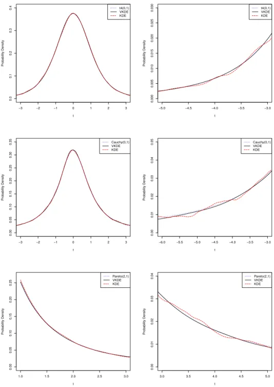
We compare the performance of VKDE and KDE by conducting simulation study of t-distribution (t4(0,1)), Cauchy(0,1) and Pareto(0,1).
The sample size is n = 50,000 for each simulation study. For all the simulations, we use KDE as in (1.1.1) with the normal kernel function. We use the code density() in the programming software R and the default bandwidth chosen by R in the estimation fort4(0,1). For Cauchy(0,1) or Pareto(0,1), the code density() in R can not provide a classical kernel density estimate. Instead, we make new code and select the bandwidth which optimizes the performance among a variety of bandwidths. For VKDE, we assume that h1,n =n−1/5, h2,n =n−1/9, and use the Tricube kernel:
K(u) = 70
81(1− |u| 3)31
|u|≤1
in either the pilot kernel density estimator or the true estimator (1.2.8). The following five time differentiable clipping function pwith t0 = 2 ([10]) is applied:
p(t) = 1 + 64t6 1−2(t−2) + 94(t−2)2− 7 4(t−2) 3+7 8(t−2) 4 if 0≤t≤2 t if t ≥2 1 if t ≤0 .
The simulation study in Figure 2.5.1 shows that, for each of these three distributions, VKDE has better performance than KDE, especially in the tail area.
−3 −2 −1 0 1 2 3 0.0 0.1 0.2 0.3 0.4 t Probability Density t4(0,1) VKDE KDE −5.0 −4.5 −4.0 −3.5 −3.0 0.000 0.005 0.010 0.015 0.020 0.025 0.030 t Probability Density t4(0,1) VKDE KDE −3 −2 −1 0 1 2 3 0.00 0.05 0.10 0.15 0.20 0.25 0.30 0.35 t Probability Density Cauchy(0,1) VKDE KDE −6.0 −5.5 −5.0 −4.5 −4.0 −3.5 −3.0 0.00 0.01 0.02 0.03 0.04 0.05 t Probability Density Cauchy(0,1) VKDE KDE 1.0 1.5 2.0 2.5 3.0 0.00 0.05 0.10 0.15 0.20 0.25 t Probability Density Pareto(2,1) VKDE KDE 3.0 3.5 4.0 4.5 5.0 0.00 0.01 0.02 0.03 0.04 t Probability Density Pareto(2,1) VKDE KDE
Figure 2.5.1: The probability density functions of t-distribution (t4(0,1)), Cauchy(0,1) and Pareto(0,1), the kernel density estimates (KDE), and the variable kernel density estimates (VKDE) with 50,000 observations generated from t-distribution (t4(0,1)), Cauchy(0,1) and Pareto(0,1) distribution. The left one shows the estimate in the main area with the mode. The right one shows the estimate in the tail area.
3 VARIABLE BANDWIDTH KERNEL REGRESSION ESTIMATION
Chapter 3 is devoted to developments of variable bandwidth kernel regression esti-mators.
3.1 DECOMPOSITION FOR KERNEL REGRESSION ESTIMATION
LetXi ∈R.
Similar to δ in Section 2.1, define δr(t) =δr(t, n) by the equation
δr(t) = α(ˆg(t;h1,n))−α(g(t)) α(g(t)) . Then, α(ˆg(t;h1,n)) = α(g(t))(1 +δr(t)) (3.1.1) Moreover, we have δr(t) = α0(g(t))[ˆg(t;h1,n)−g(t)] α(g(t)) + α00(γ)[ˆg(t;h1,n)−g(t)]2 2α(g(t)) (3.1.2)
where γ = γ(t) ≥ 0 is between ˆg(t;h1,n) and g(t). Note that, since p ≥ 1 and if p0 and p00
are uniformly bounded on [0,∞), we have |α00(γ(t, h1,n))| ≤c−3A2 for some constant A2 that
DefineD2(t;h1,n) = ˆg(t;h1,n)−E(ˆg(t;h1,n)) and b2(t;h1,n) =E(ˆg(t;h1,n))−g(t).By [24] (Theorem 3.3) and [5], sup t∈R b2(t;h1,n) =O(h21,n), (3.1.3) and sup t∈R |D2(t;h1,n)|=Oa.s. s logn nh1,n ! . (3.1.4)
Note that for d= 1, by (2.1.5), qnhlogn
1,n +h 2 1,n =U(h1,n). Then, we have, sup t∈R |δr(t)|= sup t∈R |gˆ(t;h1,n)−g(t)|= sup t∈R |D2(t;h1,n) +b2(t;h1,n)|=Oa.s.(U(h1,n)), (3.1.5) for f, r ∈ PC,2. Recall L1(t) =tK0(t) and L(t) =K(t) +L1(t), t∈R. (3.1.6)
We then have the following Taylor expansion
K t−Xi h2,n α(ˆg(Xi;h1,n)) =K t−Xi h2,n α(g(Xi)) (3.1.7) +K0 t−Xi h2,n α(g(Xi)) (t−Xi) h2,n α(g(Xi))δr(Xi) +δ3(t;Xi), where δ3(t, Xi) = K00(ξ) (t−Xi)2 2h2 2,n α2(g(Xi))δr2(Xi), ξbeing a number between t−Xi
h2,n α(g(Xi)) and t−Xi
h2,n α(g(Xi))(1+δr(Xi)). By the similar analysis
as that forδ2 in Section 2.1
sup
t,x∈R
|δ3(t, x)|=Oa.s. kgˆ(·;h1,n)−g(·)k2∞
iff, r ∈ PC,2. Therefore, by using the expansion (3.1.1) ofα( ˆf), the Taylor expansion (3.1.7),
and the notations L1 and Lin (3.1.6), we get
ˆ g(t;h1,n, h2,n) =¯g(t;h2,n) + 1 nh2,n n X i=1 L t−Xi h2,n α(g(Xi)) α(g(Xi))δr(Xi)Yi + 1 nh2,n n X i=1 L1 t−Xi h2,n α(g(Xi)) α(g(Xi))δ2r(Xi)Yi + 1 nh2,n n X i=1 α(g(Xi))δ3(t, Xi)δr(Xi)Yi + 1 nh2,n n X i=1 α(g(Xi))δ3(t, Xi)Yi. (3.1.9)
3.2 BIAS OF VARIABLE BANDWIDTH KERNEL REGRESSION ESTIMATOR
3.2 Ideal Estimator
Forr1 >0, 1≤t0 <∞, and c >0, define Drf =D1∩D2, where
D1 ={t ∈R:f(t)> r1 > t0c2, |t|<1/r1}, D2 ={t∈R:g(t)> r1 > t0c2, |t|<1/r1} Recall that ¯ r(t;hn) = 1 nhn Pn i=1K t−Xi hn α(g(Xi)) α(g(Xi))Yi 1 nhn Pn i=1K t−Xi hn α(f(Xi)) α(f(Xi)) = g¯¯(t;hn) f(t;hn). (3.2.1)
Consider bias of the ideal variable bandwidth regression estimator (3.2.1) at a fixed point
t ∈ Drf. The rate of convergence of this bias depends on the properties of f, r, and the
clipping function p.
Assumptions 3. The sequence hn satisfies the following classical conditions:
hn&0,
nhn
|loghn| → ∞,
|loghn|
log logn → ∞, and nhn % ∞,
as n → ∞. K is non-negative, symmetric about zero, and has bounded and continuous
second order derivatives. Assume that K has support [−T, T] for some T < ∞. Set α(x) =
cp1/2(c−2x)for x∈R and some c >0 . Moreover, letr be bounded function with r∈C4(R).
The following proposition and its proof are contained in [17] and [15] (see also the theorem in [11]). We require this proposition to prove Theorem 3.2.5, more specifically to work on E(¯g) and E( ¯f).
Proposition 3.2.1 ([17]). Assume that K is a symmetric kernel and has bounded support
in [−T, T]. Let η be a function in Cl(R) and ξ a function in Cl+1(R). Assume ξ(t)≥c >0
for some c >0 and all t ∈R. Then,
1 h Z K t−s h ξ(s) ξ(s)η(s)ds= l X k=0 ak(t)hk+o(hl)
as h→0, uniformly for t ∈R , and the set of functions ak(t), which are uniformly bounded
and equicontinuous, are defined as
a2k+1(t) = 0, a2k(t) = ρ2k (2k)!D2k η(t) ξ2k(t) ,
fork ≤l/2, in particular, a0(t) =η(t). Hereρk=
R
wkK(w)dwandD
k is thekthderivative.
The following three lemmas are necessary to establish our results on the bias of ¯